Practical Poissonian-Gaussian noise modeling and fitting for single ...

IEEE TRANSACTIONS, TIP-03364-2007-FINAL

1

Practical Poissonian-Gaussian noise modeling and Þtting for single-image raw-data Alessandro Foi, Mejdi Trimeche, Vladimir Katkovnik, and Karen Egiazarian, Senior member, IEEE

Abstract— We present a simple and usable noise model for the raw-data of digital imaging sensors. This signal-dependent noise model, which gives the pointwise standard-deviation of the noise as a function of the expectation of the pixel raw-data output, is composed of a Poissonian part, modeling the photon sensing, and Gaussian part, for the remaining stationary disturbancies in the output data. We further explicitly take into account the clipping of the data (over- and under-exposure), faithfully reproducing the nonlinear response of the sensor. We propose an algorithm for the fully automatic estimation of the model parameters given a single noisy image. Experiments with synthetic images as well as with real raw-data from various sensors prove the practical applicability of the method and the accuracy of the proposed model. Index Terms— clipping, digital imaging sensors, noise estimation, noise modeling, overexposure, Poisson noise, raw-data.

I. I NTRODUCTION Progress in hardware design and manufacturing has introduced digital imaging sensors having a dramatically increased resolution. This is mainly achieved by an increase of the pixel density. Despite the electrical and thermal characteristics of the sensors have noticeably improved in the last decade [18], [15], with the size of each pixel becoming smaller and smaller the sensor output signal’s susceptibility to photon noise has become greater and greater. As of now, this source of noise appears as the most signiÞcant contributor of the overall noise in a digital imaging sensor [1]. This makes the noise component of the raw-data output of the sensor markedly signal-dependent, thus far from the conventional additive white Gaussian noise modeling so widely used in image processing. Further, with the intention of making full use of the rather limited dynamic range of digital sensors, pictures are usually taken with some areas purposely overexposed or clipped, i.e. accumulating charge beyond the full-well capacity of the individual pixels. These pixels obviously present highly nonlinear noise characteristics, which are completely different than those of normally exposed pixels. The raw-data which comes from sensor always undergoes various processing stages (e.g., denoising, demosaicking, deblurring, compression) before the Þnal “cooked” image reaches the user. In order to process the data and/or to attenuate A. Foi, V. Katkovnik, and K. Egiazarian are with the Department of Signal Processing, Tampere University of Technology, P.O. Box 553, 33101 Tampere, Finland. E-mail: Þrstname.lastname@tut.Þ M. Trimeche is with the Multimedia Technologies Laboratory, Nokia Research Center, Tampere, Finland, E-mail: Þ[email protected] This work was supported by the Finnish Funding Agency for Technology and Innovation (Tekes), AVIPA/AVIPA2 projects, and by the Academy of Finland, project No. 213462 (Finnish Centre of Excellence program 2006 2011).

the noise in the most efÞcient and effective way, it is vital that a proper modeling of the noise is considered during the various stages of digital image processing. However, the technical datasheets of the devices usually provide vague and inadequate Þgures for the noise that are of a global nature (i.e., “average” values which are meant to be valid for the whole sensor) [17]. Consequently, raw-data Þltering algorithms either assume independent stationary noise models or, if a signal-dependent model is assumed, the correct parameters for the noise are often not speciÞed. Such rough noise estimates are inadequate for the high-quality image processing Þlters which are rapidly becoming an integral part of the imaging chain. Two are the contributions in this paper. First, we present a simple noise model which can accurately be used for the raw-data. Based on the above considerations, it is a signaldependent noise model based on a Poissonian part, modeling the photon sensing, and Gaussian part, for the remaining stationary disturbances in the output data. We explicitly take into account the problem of clipping (over- and under-exposure), faithfully reproducing the nonlinear response of the sensor. Only two parameters are sufÞcient to fully describe the model. These parameters are explained in relation to the sensor’s hardware characteristics (quantum efÞciency, pedestal, gain). As a second and most important contribution, we propose an algorithm for the fully automatic estimation of the model parameters given a single noisy image. The paper is organized as follows. In Section II we present the model in its basic form, which ignores the clipping. The parameter estimation algorithm is then presented in Section III. The general model with clipping requires more involved mathematics, and it is given in Section IV, followed by the modiÞed estimation algorithm in Sections V and VI. Throughout these sections, we demonstrate the accuracy of the algorithm with synthetic test images, for which the exact noise parameters are known. Experiments with real raw-data are presented in Section VII; these experiments prove the practical applicability of the method and conÞrm that the raw-data noise can indeed be accurately modeled as a clipped Poissonian-Gaussian process. Further comments and details on the algorithm and its implementation are given in Section VIII. II. P OISSONIAN -G AUSSIAN MODELING Let us consider the generic signal-dependent noise observation model of the form z (x) = y (x) + σ (y (x)) ξ (x) (1) where x ∈ X is the pixel position in the domain X, z : X → R is the observed (recorded) signal, y : X → R is the original

2


(unknown) signal, ξ : X → R is zero-mean independent random noise with standard deviation equal to 1, and σ : R → R+ is a function of y that gives the standard deviation of the overall noise component. Throughout the paper, we denote the expected value (or mathematical expectation) of a random variable as E {·}, itspvariance as var {·}, and its standard deviation as std {·} = var {·}; when any of these operators is applied to a sequence (resp. matrix) of random variables, its output is deÞned as the sequence (resp. matrix) of the operator’s outputs for the individual random variables. The symbol σ is used exclusively to denote this function of the model (1). From E {ξ (x)} = 0 follows that E {z (x)} = y (x), i.e. the original signal can be deÞned as the expected value of the noisy observations. Consequently, we have that std {z (x)} = σ (E {z (x)}), i.e. the standard deviation of the noise is a function, namely σ, of the expectation of the noisy signal. In our modeling, we assume that the noise term is composed of two mutually independent parts, a Poissonian signaldependent component η p and a Gaussian signal-independent component ηg : σ (y (x)) ξ (x) = η p (y (x)) + η g (x) . (2) In terms of distributions, these two components are characterized as follows, ¡ ¢ χ y (x) + η p (y (x)) ∼ P (χy (x)) , η g (x) ∼ N (0, b) , where χ > 0 and b ≥ 0 are real scalar parameters and P and N denote the Poisson and normal (i.e., Gaussian) distributions. From the elementary properties of the Poisson distribution, we obtain the following equation for the mean and variance © ¡ ¢ª © ¡ ¢ª E χ y (x) + η p (y (x)) = var χ y (x) + η p (y (x)) =

= χy (x) . ¢ª © ª © ¡ = χy (x) + χE ηp (y (x)) Since E χ© y (x) + ηª p (y (x)) and χ2 var ηp (y (x)) = χy (x), it follows that © ª © ª E ηp (y (x)) = 0 and var η p (y (x)) = y (x) /χ. Thus, the Poissonian η©p has varying ª variance that depends on the value of y (x), var ηp (y (x)) = ay (x), where a = χ−1 . The Gaussian component ηg has instead constant variance equal to b. Consequently, the overall variance of z in (1) has the afÞne form σ2 (y (x)) = ay (x) + b,

(3)

which gives the standard deviation σ as the square root p σ (y (x)) = ay (x) + b, (4) √ √ and, in particular, σ (0) = b and σ (1) = a + b. Some examples of standard-deviation functions σ for different combinations of the constants a and b are shown, as an illustration, in Figure 1 (solid lines). Figure 2 presents a simple piecewise smooth image which is degraded by Poissonian and Gaussian noise with parameters χ = 100 (a = 0.01) and b = 0.042 . As illustrated in Figure 1, these parameters imply that the noise standard-deviation in the brightest parts of the image is more than twice as large as in the darker ones.

A. Raw-data modeling The Poissonian-Gaussian model (1-2) is naturally suited for the raw-data of digital imaging sensors. The Poissonian component η p models the signal-dependent part of the errors, which is essentially due to the photon-counting process, while the Gaussian ηg accounts for the signal-independent errors such as electric and thermal noise. We brießy mention how the above model parameters relate to elementary aspects of the digital sensor’s hardware. 1) Quantum efÞciency: The parameter χ of η p is related to the quantum efÞciency of the sensor: the larger the number of photons necessary to produce a response of the sensor (generation of an electron), the smaller the χ. 2) Pedestal parameter: In digital imaging sensors, the collected charge is always added to some base “pedestal” level p0 ∈ R+ . This constitutes an offset-from-zero of the output data and it can be rewritten as a shift in the argument of the signal-dependent part of the noise: z (x) = y (x) + σ (y (x) − p0 ) ξ (x) = = y (x) + η p (y (x) − p0 ) + ηg (x) .

3) Analog gain: We model the analog gain as an ampliÞcation of the collected charge. Let us denote the variables before ampliÞcation by the circle superscript û, û z (x) = û y (x) + û ηp (û y (x) − p0 ) + û ηg (x) . We formalize the ampliÞcation Θ of û z as the multiplication of the noise-free signal, of the Poissonian noise, and of a part of the Gaussian noise, by a scaling constant θ > 1, ¡ ¢ z(x) = Θ (û z (x)) = θ û y(x) + û η p (û y (x)−p0 ) + û η 0g(x) +û η00g (x). Here, the Gaussian noise term û η g has been split in two η 00g , û η0g +û η00g = ηg , where û η00g represents the components û η0g and û portion of the noise that is introduced after the ampliÞcation and thus not affected by the factor θ. The expectation and variance for z are E {z (x)} = y (x) = θû y (x) ,

var {z (x)} = © 0 ª © 00 ª = θ χ (û y (x) − p0 )+θ var û ηg (x) +var û η g (x) . Hence, we come again to a model of the form (3)-(4) with © 0 ª © 00 ª a = χ−1 θ, b = θ2 var û η g (x) + var û ηg (x) − θ2 χ−1 p0 . Note that now this b can be negative, provided a large pedestal p0 and a small variance of û ηg . This does not mean that there is a “negative” variance. Indeed, because of the pedestal, y ≥ θp0 and therefore ay + b ≥ 0. In digital cameras, the analog gain (i.e., θ) is usually controlled by the choice of the ISO sensitivity setting. This can be done manually by the user, or automatically by the camera (“auto mode”). Large ISO numbers (e.g., 800 or 1600) correspond to large θ, and thus worse signal-to-noise ratio (SNR). Lower values (e.g., ISO 50) yield a better SNR but at the same time produce darker images, unless these are taken with a longer exposure time (which corresponds to having larger values of û y before the multiplication by θ). Figure 3 shows few examples of the standard-deviation functions σ which can typically be found for the raw data. Two of these examples have b < 0, which corresponds to a pedestal p0 > 0. 2 −1

2

FOI ET AL., PRACTICAL POISSONIAN-GAUSSIAN NOISE MODELING AND FITTING FOR SINGLE-IMAGE RAW-DATA

3

Fig. 1. Some examples of the standard-deviation functions σ (solid lines) from the model (1) for different combinations of the constants a and b of Equation (4): (left) a = 0.022 , 0.062 , 0.102 , b = 0.042 and (right) a = 0.42 , b = 0.022 , 0.062 , 0.102 . The dashed lines show the corresponding functions σ ˜ of the clipped observation model (30), as functions of the clipped y˜ (see Section IV). The small black triangles indicate the points (˜ y, σ ˜ (˜ y)) which correspond to y = 0 and y = 1.

Fig. 2. A piecewise smooth test image of size 512 × 512: original y and observation z degraded by Poissonian and Gaussian noise with parameters χ = 100 (a = 0.01) and b = 0.042 .

B. Heteroskedastic normal approximation Throughout the following sections, we need to derive a few results and relations which depend not only on the mean and variance, but also on the particular distribution of the processed samples. For the sake of simpliÞcation, we exploit the usual normal approximation of the Poisson distribution, which gives P (λ) ≈ N (λ, λ) . (5) The accuracy of this approximation increases with the parameter λ and in practice, for large enough1 λ, a Poissonian process can be treated as a special heteroskedastic Gaussian one. We thus obtain the following normal approximations of the errors p σ (y (x)) ξ (x) = ay (x) + bξ (x) ' ηh (y (x)) , (6) where η h (x) ∼ N (0, ay (x) + b). III. T HE ALGORITHM Our goal is to estimate the function σ : R → R+ of the observation model (1) from a noisy image z. The proposed algorithm is divided in two main stages: local estimation of multiple expectation/standard-deviation pairs and global parametric model Þtting to these local estimates. An initial 1 How large λ is enough really depends on the considered application and desired accuracy. The fact that the Poisson distribution is discrete is a secondary aspect, because quantization of the digital data makes anyway discrete even errors due to continuous distributions. For the considered standard-deviation estimation problem, we found experimentally that already with λ = 10 (corresponding to χ = 20 for the middle intensity y = 0.5) there is virtually no difference between the estimation accuracy of a truly Poissonian variable and that of its Gaussian approximation.

Fig. 3. Some examples of the standard-deviation functions σ (solid lines) which are often found for the! raw data. In these"three ! examples the parameters " (a, from Equation (4) are 1.5 · 10−3 , 10−4 , 6 · 10−4 , −5 · 10−6 , and " ! b) ˜ of 10−4 , −8 · 10−6 . The dashed lines show the corresponding functions σ the clipped observation model (30), as functions of the clipped y˜ (see Section IV). The small black triangles indicate the points (˜ y, σ ˜ (˜ y)) which correspond to y = 0 and y = 1.

preprocessing stage, in which the data is transformed to the wavelet domain and then segmented into non-overlapping level sets where the data is smooth, precedes the estimation. A. Wavelet domain analysis Similar to [4], we facilitate the noise analysis by considering wavelet detail coefÞcients z wdet deÞned as the downsampled convolution z wdet =↓2 (z ~ ψ) , where ψ is Pa 2-D wavelet function with zero mean and unity ψ = 0, kψk2 = 1, and ↓2 denotes the decimation 52 -norm, operator that discards every second row and every second column. Analogously, we deÞne the normalized approximation coefÞcients as z wapp =↓2 (z ~ ϕ) , where ϕ is the corresponding 2-D wavelet scaling function, P which we specially normalize so that ϕ = 1. For noisy images, the detail coefÞcients z wdet contain mostly noise and, due to the normalizations of the convolution kernels, we have µq ¶ © wdet ª 2 std z var {z} ~ ψ ' (7) = ↓2 (std {z ~ ψ}) =↓2 ' ↓2 (std {z} kψk2 ) =↓2 (std {z}) = P = ↓2 (σ (y)) = σ (↓2 y) = σ (↓2 (y ϕ)) ' ' σ (↓2 (y ~ ϕ)) = σ (E {z wapp }) , (8)

4


Fig. 4. From left to right: wavelet approximation and detail coefÞcients z wapp and z wdet , restricted on the set of smoothness X smo , and two level-sets Si (13) computed for ∆i = ∆ = 1/300. The scale of this Þgure is half that of Fig. 2.

with the approximate equalities ' becoming accurate at points in regions where y (and hence std {z}) is uniform, as we can assume that the distribution of z does not change over the small support of the wavelets. Thus, in particular, at a point x in such uniform regions, we can assume that z wdet (x) ∼ N (0, σ (E {z wapp (x)})) , (9) and, because of decimation and orthogonality properties of wavelet functions, that the noise degrading z wdet , as well as the noise degrading z wapp , are independent ones. Note that, always, kϕk2 6= 1. Therefore, when considering std {z wapp }, the above equations can be repeated, replacing ψ with ϕ, only provided that the factor kϕk2 is kept. Thus, we come to std {z wapp } ' kϕk2 σ (z wapp ) . In our implementation, we use separable kernels ψ = ψ 1 ~ ψ T1 and ϕ = ϕ1 ~ ϕT1 where ψ 1 and ϕ1 are 1-D Daubechies wavelet and scaling functions

ψ1 = [0.035 0.085 − 0.135 − 0.460 0.807 − 0.333] , (10) ϕ1 = [0.025 − 0.060 − 0.095 0.325 0.571 0.235] .

B. Segmentation Like in our previous work [6], we segment the data into level sets, in each of which the image can be reasonably assumed to be uniformly close to a certain value. Having nothing but a noisy image at our disposal, we shall employ spatial smoothing (as opposed to temporal smoothing, used in [6]) in order to attenuate the noise and an edge-detector in order to stay clear from edges when analyzing the data, thus enabling the conditions (7)-(8). There exist a myriad of different methods which can be used for smoothing or for edge detection. However, for our purposes, the following simple and non-adaptive methods proved adequate for all considered experimental cases. 1) Smoothed approximation: From z wapp , we compute a smoothed (low-pass) image z smo , z smo = z wapp ~ 7, (11) where 7 is positive smoothing kernel, 7 ≥ 0 and k7k1 = 1. The smoothing action of the kernel should be especially strong, so to effectively suppress most of the noise. In our implementation, we use a uniform 7 × 7 kernel for 7. In the corresponding regions where y itself is smooth, z smo is approximately equal to E {z wapp }, and thus to ↓2 y. This is

a reasonable assumption provided that the support of 7 does not intersect edges during the calculation of the convolution (11). 2) Edges and set of smoothness: To detect edges, we use the conventional approach where some smoothed derivatives of the image are thresholded against an estimate of the local standard deviation. Exploiting the fact thatpthe mean of the absolute deviations of N (0, 1) is equal to 2/π [7], we can deÞne a rough estimate of the local standard-deviations of z wdet as the map r π ¯¯ wdet ¯¯ z s= ~ 7. 2 We deÞne the set of smoothness X smo as X smo = {x ∈↓2 X : : |∇ (Λ (z wapp )) (x)| + |Λ (z wapp ) (x)| < τ · s (x)}, Λ (z 2

wapp

2

) = ∇ medÞlt (z

wapp

(12)

),

where ∇ and ∇ are, respectively, gradient and Laplacian operators, medÞlt denotes a 3 × 3 median Þlter, ↓2 X is the decimated domain of the wavelet coefÞcients z wapp , and τ > 0 is positive threshold constant. We realize both the Laplacian operator ∇2 and the gradient operator ∇ as convolutions against 9 × 9 kernels. Thresholding the sum of the moduli of the Laplacian and of its gradient is a heuristic way to obtain “thickened” edges. In Figure 4, we show the wavelet approximation and detail coefÞcients z wapp and z wdet , restricted on the set of smoothness X smo (whose complement thus appears as white in the Þgure), calculated for the test image z of Figure 2. Note that some of the weakest edges have not been detected as such. 3) Level sets (segments): In the set of smoothness X smo , we can assume that edges of the image did not interfere with the smoothing (11), hence, that the conditions (7)-(8) hold and that, for x ∈ X smo , z smo (x) = E {z wapp (x)} = E {(↓2 z)(x)} = (↓2 y)(x) , © ª std z wdet (x) = std {(↓2 z)(x)} = (↓2 (σ (y)))(x).

We identify in the smoothness set X smo a collection of N non-overlapping level sets (segments) Si ⊂ X smo , i = 1, . . . , N of the smoothed image z smo . Each level set, characterized by its centre value ui and allowed deviation ∆i > 0, is deÞned as Si = {x ∈ X smo : z smo (x) ∈ [ui − ∆i /2, ui + ∆i /2)} . (13)


By non-overlapping we mean that Si ∩ Sj = ∅ if i 6= j. In practice, assuming a signal in the range [0, 1], one can take Þxed §∆i ¨ª ≡ ∆ and equispaced ui ∈ © ¯ = ∆−1 , where the b·c brackets indi∆j, j = 1, . . . , N cate the rounding to the nearest larger or equal integer. Further, we require that the level sets are non-trivial, in the sense that ¯ eachSset Si must contain at least two samples2 ; thus, N ≤ N N smo and i=1 Si ⊆ X ⊆↓2 X. Figure 4 shows two of the level sets computed for the example in Figure 2 for ∆ = 1/300. Observe that these sets are meager and quite fragmented. C. Local estimation of expectation/standard-deviation pairs For each level set Si , we deÞne the (unknown) variable ni 1 X ni yi = E {z wapp (xj )} , {xj }j=1 = Si . (14) ni j=1

Note that yi and ui might not coincide. The level set Si is used as a one domain for the computation of a pair of estimates (ˆ yi , σ ˆ i ), where yî is an estimate of yi and σ ˆ i is an estimate of σ (yi ). In what follows, although we shall refer explicitly to yi , this variable is always used implicitly and, in the Þnal estimation of the function y 7→ σ (y), the many yi , i, . . . , N , remain “hidden” variables which are modeled as unknown. Similarly, the smoothed data z smo and the values ui and ∆i used for the construction of Si do not appear in the following estimation, where only z wdet , z wapp and Si are used in order to compute the estimates yî and σ î. 1) Estimation of yi : We estimate yi as the sample mean of the approximation coefÞcients z wapp on Si ni 1 X ni yî = z wapp (xj ) , {xj }j=1 = Si . (15) ni j=1

ˆ i is calculated as the 2) Estimation of σ (yi ): The estimate σ unbiased sample standard-deviation of the detail coefÞcients z wdet on Si sP ¢2 ni ¡ wdet (xj ) − z¯iwdet 1 j=1 z σ î = , (16) κni ni − 1 P i z wdet (xj ) and the factor κ−1 where z¯iwdet = n1i nj=1 ni is deÞned [7] ¡ ¢ r µ ¶ Γ n2 1 2 1 7 ¡ n−1 ¢ = 1 − + O κn = . (17) − n−1Γ 2 4n 32n2 n3 This factor, which comes from the mean of the chi-distribution with n − 1 degrees of freedom, makes the estimate unbiased for normally and identically independently distributed (i.i.d.) z wdet (xj ). 3) Unbiasedness: Clearly from the deÞnition (14), yî is an unbiased estimator of yi . The unbiasedness of σ ˆ i as an estimator of σ (yi ) is a more complex issue. As observed above, σ ˆ i is an unbiased estimator of σ (yi ) provided that z wdet is normally i.i.d. on the level set Si . However, we cannot claim, in general, that z wdet is identically distributed on Si . We remark that 2 The smoothness threshold τ (12) can be automatically increased in the rare event of N < 2, i.e. when there are not enough non-trivial level sets for the estimation. Note that X smo is monotonically enlarging to ↓2 X with τ , X smo % ↓2 X. τ →∞

5

the assumed validity of (7)-(8) concerns individual points. © ª It does not mean that std z wdet is constant over Si . As a matter of fact, especially for large ∆i , E {z wapp (x)} is not constant for x ∈ Si , which implies that the standard deviations of the wavelet detail coefÞcients (8) are not constant over Si . Lacking any particular hypothesis on the image y, it is nevertheless reasonable to assume that {E {z wapp (x)}, x ∈ Si } has a symmetric (discrete) distribution centred at yi (with diameter ©bounded by ª ∆i ). Because of (3) and (9), we have that {var z wdet (x) , x ∈ Si } has also a symmetrical distribution, which is centred at var {yi }. This makes κ2ni σ ˆ 2i 3 an unbiased estimator of var {yi } and, since κn → 1, n→∞ σ ˆ i is an asymptotically unbiased estimator of σ (yi ). This asymptotic unbiasedness is relevant in the practice, since a large ∆i corresponds to large ni . We further note that, despite the segmentation and removal of edges, the presence of sharp image features, singularities, or even texture in the segment Si is not completely ruled out. This can be effectively compensated by means of non-linear robust estimators of the standard deviation, such as the well-known median of absolute deviations (MAD) [12]. For the sake of expository simplicity, in the current and in the next section we restrict ourself to the basic estimator (16) and postpone considerations on robust estimation of the standard-deviation to Section VI. 4) Variance of the estimates: The variance of the estimates yî and σ ˆ i depends directly on the variances of the samples used for the estimation, which are degraded by independent noise. With arguments similar to Section III-C.3, the variances of the estimates can be expressed as var {ˆ yi } = σ 2 (yi ) ci , var {ˆ σ i } = σ 2 (yi ) di , (18) µ ¶ 2 2 1 − κni kϕk2 1 5 1 ci = , di = = + 2 + O 3 , (19) 2 ni κni 2ni 8ni ni where these expressions coincide with those for the perfect © ª case when var z wdet and var {z wapp } are constant on Si [7]. î 5) Distribution of the estimates: The estimates yî and σ are distributed, respectively, following a normal distribution and a scaled non-central chi-distribution, which can also be approximated, very accurately for large ni , as a normal distribution [7]. Thus, in what follows, we treat both yî and σ ˆ i as normally distributed random variables and, in particular, as ¢ ¢ ¡ ¡ yî ∼ N yi , σ 2 (yi ) ci , σ ˆ i ∼ N σ (yi ) , σ 2 (yi ) di , (20) where ci and di are deÞned as in (19). D. Maximum-likelihood Þtting of a global parametric model The maximum-likelihood (ML) approach is used to Þt a global parametric model of the function σ on the estimates N ˆ i }i=1 . Depending on the parameters a and b, we have {ˆ yi , σ 2 σ (y) = ay + b. For reasons of numerical consistency (note that formally this σ 2 (y) may be zero or negative), for the Þtting we deÞne a simple regularized variance-function σ 2reg as ¡ ¢ σ 2reg (y) = max ε2reg , σ 2 (y) (21) 3 This

as zero.

# $ can be proved easily since, for x ∈ X smo , we can treat E z wdet (x)

6


From (23), the sought parameter estimates a ˆ and ˆb are deÞned ³ ´ as the solution of a ˆ, ˆb = argmax L (a, b) = argmin − ln L (a, b) = (24) a,b

a,b

Z N X = argmin − ln ℘ ((ˆ yi , σ ˆ i ) |yi = y) ℘0 (y) dy. a,b

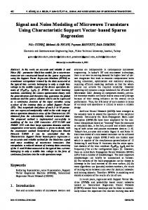
Fig. 5. Each dot of the scatter plot corresponds to a pair (ˆ yi , σ ˆ i ) of estimates of yi and σ (yi ). The solid line shows the maximum-likelihood estimate σ ˆ Þt of the true standard-deviation function σ. The plot of σ ˆ Þt overlaps perfectly with that of the true σ (shown in Figure 1). The estimated parameters are % a ˆ = 0.01008 (ˆ χ = 99.20) and ˆb = 0.001583 ( ˆb = 0.03979). The initialization parameters, found as the least-squares ˆ0 = % solution (26), were a 0.00994 (ˆ χ0 = 100.62) and ˆb0 = 0.001649 ( ˆb0 = 0.04061).

where εreg > 0 is a small regularizationqparameter. Hence, the regularized standard-deviation σ reg = σ 2reg (y) is always well deÞned, for any choice of a, b, and y. As discussed in Section III-C.5, we can assume normality ˆ i . Thus, the conditional and unbiasedness for both yî and σ probability densities of yî and σ ˆ i given yi = y are, respectively, − 2σ2 1(y)c i reg

1 e 2πσ 2reg (y)ci

℘ (ˆ yi |yi = y) =

√

℘ (ˆ σi |yi = y) =

√

2

(ˆ yi −y)

,

− 2σ2 1(y)d (ˆ σ i −σ reg (y))2 1 i reg e . 2 2πσ reg (y)di

Further, we observe that, because of the orthogonality of the ˆ i are mutually independent4 . Hence, wavelets, yî and σ ℘ ((ˆ yi , σ ˆ i ) |yi = y) = ℘ (ˆ yi |yi = y) ℘ (ˆ σ i |yi = y) = (22) !

y ˆ −y 2

(y) 2

"

( ( i ) ) reg − 2σ21 (y) + i d 1 1 ci i reg = √ . e 2π ci di σ 2reg (y) The posterior likelihood L is obtained by considering all ˆ i )}N measurements {(ˆ yi , σ i=1 and by integrating the densities ℘ ((ˆ yi , σ ˆ i ) |yi = y) with respect to a prior probability density ℘0 (y) of y, N Z ∞ Y ℘ ((ˆ yi , σ ˆ i ) |yi = y) ℘0 (y) dy. (23) L (a, b) = σ ˆ −σ

i=1

Hence, our Þnal estimate of the function σ is r ³ ´ ˆy + ˆb . σ ˆ Þt (y) = max 0, a

(25)

Figure 5 shows the result of the above optimization for the test example shown in Figure 2. It can be seen that the procedure estimates the parameters of the noise with great accuracy. 1) Iterative solution and initialization: In our implementation, we solve the problem (24) numerically, using the NelderMead iterative downhill simplex method [13] and evaluating the integrals as Þnite sums. As initial parameters a ˆ0 , ˆb0 for this iterative optimization we take the least-squares solution h i ¢¡ ¢T ¡ v [a b] ΦT −ˆ v = (26) a ˆ0 , ˆb0 = argmin [a b] ΦT −ˆ a,b

where 

¢−1 ¡ , = v ˆΦ ΦT Φ

yˆ1  yˆ2 Φ = .. .

 1 1  , .. .

v ˆ=

(27)

£

κ ÿ 2n1 σ ˆ 21

κ ÿ 2n2 σ ˆ 22

···

¤

, (28)

ÿ n = κn . The linear problem with the factors κ ÿ n deÞned as κ (26) allows a simple direct solution by means of the normal equations (27). While in (24) we aim at Þtting the standardN deviation curve σreg to the estimates {(ˆ yi , σ ˆ i )}i=1 , Equation (26) minimizes the residuals with respect to the variances σ ˆ2, treated as a linear function of the parameters a and b. Here, the factor κ ÿ 2ni makes κ ÿ 2ni σ ˆ 2i an unbiased estimate of the variance (contrary to σ ˆ i (16), which is an unbiased estimate of the standard deviation). IV. C LIPPING ( CENSORING ) A. Clipped observations model

The integration copes with the fact that yi and y are unknown. For images in the range [0, 1], the simplest and most obvious choice is ℘0 to be uniform Ron [0, 1], which implies that (23) QN 1 yi , σ ˆ i ) |yi = y) dy. In our becomes L (a, b) = i=1 0 ℘ ((ˆ experiments with synthetic images we use this prior. However, we wish to note that other prior statistics have been shown to be more representative of the histograms of natural images [10]. Let us observe that (ˆ yi , σ ˆ i ) and (ˆ yj , σ ˆ j ) , i 6= j, are mutually independent because the corresponding level sets Si and Sj are non-overlapping.

In practice, the data range, or dynamic range, of acquisition, transmission, and storage systems is always limited. Without loss of generality, we consider data given on the normalized range [0, 1], where the extremes correspond to the maximum and minimum pixel values for the considered noisy image (e.g., raw data) format. Even if the noise-free image y is within the [0, 1] range, the noise can cause z to exceed these bounds. We shall assume that values exceeding these bounds are replaced by the bounds themselves, as this corresponds to the behavior of digital imaging sensors in the case of overor underexposure. Thus, we deÞne the clipped (or censored5 )

4 This independence is a general property of the sample mean and sample standard-deviation, which property holds also when the estimates are computed from the very same samples [7]. However, by sampling two independent sets of wavelet coefÞcients, we have that the two estimates are necessarily independent, regardless of the particular mean and standarddeviation estimators used, a fact that comes useful for the forthcoming sections.

5 Strictly speaking, the form of the so-called censored samples [2] is really z˜ = z if 0 ≤ z ≤ 1 and no sample (i.e., censoring) if z < 0 or z > 1. Usually, the amount of censored samples below and above the extrema are assumed as known (Type-1 censoring). Thus, clipped (29) and censored observations can, in a sense, be considered as equivalent. However, the formulas and estimators for censored variables which can be found in the literature cannot be used directly in the case of the clipped observations (29).

i=1

−∞


observations z˜ as z˜ (x) = max (0, min (z (x) , 1)) , x ∈ X, (29) where z is given by the signal-dependent noise model (1). Let y˜ (x) = E {˜ z (x)}. The corresponding noise model for the clipped observations (29) is z˜ (x) = y˜ (x) + σ ˜ (˜ y (x)) ˜ξ (x) , (30) n o n o where again E ˜ξ (x) = 0, var ˜ξ (x) = 1, and the

function σ ˜ : [0, 1] → R is deÞned as σ ˜ (˜ y (x)) = std {˜ z (x)}. In general, y˜ (x) = E {˜ z (x)} 6= E {z (x)} = y (x), σ ˜ (˜ y (x)) =nstd {˜ zo(x)} 6= std {z (x)} = σ (y (x)), and, even though var ˜ξ (x) = var {ξ (x)} = 1, the distributions of ξ and ˜ξ are different. In Figure 1 one can compare the standard-deviation functions σ ˜ (dashed line) and σ (solid line) for different combinations of the constants a and b in (4). In the next sections, we rely on the heteroskedastic normal approximation (6) and hence treat z as a purely Gaussian variable. Consequently, we model z˜ as a clipped (censored) normal variable. We note that this normal approximation is especially relevant for values of y = E {z} close to 0 or 1, where the clipping effects may be dominant. For y close to 1, we have that (5) holds with the largest values of λ, hence is for this values of y that the Gaussianization of the Poissonian component η p (y (x)) is most accurate. For y close to 0, although λ in (5) might not be large, the approximation holds because the variance ay (x) of η p (y (x)) becomes negligible compared to the variance b of the Gaussian part η g (x). This is true provided that b 6= 0. However, if b = 0 the noise has only the Poissonian component η p , which is always positive. It means that z ≥ 0 and, thus, z˜ = min (1, z). Therefore, if b = 0, for our purposes it is sufÞcient to consider only the normal approximation for y close to 1, as no clipping happens at 0. +

B. Expectations, standard deviations, and their transformations To simplify the calculations, we shall assume that the two clippings, the one from below (z < 0, z˜ = 0) and the one from above (z > 1, z˜ = 1), are not mixed by the randomness of the noise, and can thus be computed independently6 . In other words, this means that, in practice, if y is close enough to 0 so that it is possible that z < 0, then it is impossible that z > 1; similarly, if y is close enough to 1, so that z can be larger than 1, then z cannot be smaller than 0; for intermediate values of y, with 0 ¿ y ¿ 1, we have that 0 < z < 1, i.e. clipping is not happening. In what follows, we therefore treat separately the two cases: 6 Formally, this corresponds to assuming that, for a given y (x), the product probability P (z (x) > 1) · P (z (x) < 0) is negligibly small. This condition is satisÞed provided, e.g., the stronger condition that P (z (x) < 0|y (x) > 1 − 4) and P (z (x) > 1|y (x) < 4) are both negligibly small for 4 = 0.5. These conditions are all surely met in the practical cases, since there the standard deviation σ (y (x)) of z (x) is always much smaller (in fact, several orders smaller) than 0.5 and its distribution does not have heavy tails (note that [y − γσ (y) , y + γσ (y)] with γ ≥ 4 can be a rather “safe” conÞdence interval for z, with higher than 99.99% conÞdence for Gaussian distributions).

7

Fig. 6. The probability density function of ν˜ = max (0, ν), as deÞned by Equation (31). In this illustration µ = 1. The height of the impulse at 0 is equal to the area under the bell curve between −∞ and 0.

• •

clipping from below (left single censoring): y and z are near 0 and z < 1, thus, z˜ = max (0, z); clipping from above (right single censoring): y and z are near 1 and z > 0, thus, z˜ = min (z, 1).

Further, we combine the results for the two cases, so to obtain formulas which are valid for the case z˜ = max (0, min (z, 1)), where clipping can happen from above or below (double censoring). 1) Clipping from below (left single censoring): Since z˜ = max (0, z), we have that E {˜ z } ≥ E {z} = y. Let ν ∼ N (µ, 1) be a normally distributed random variable with mean E {ν} = µ and unitary variance and ν˜ = max (0, ν). The probability density fν˜ of ν˜ is a generalized function deÞned as follows ½ φ (t − µ) + Φ (−µ) δ 0 (t) t ≥ 0, fν˜ (t) = (31) 0 t < 0, where φ and Φ are the probability density and cumulative distribution functions (p.d.f. and c.d.f.) of the standard normal N (0, 1) and δ 0 is the Dirac delta impulse. This function is illustrated in Figure 6. Tedious but simple calculations (see, e.g., [7], or [8], Chapter 20) show that the expectation E {˜ ν } and the variance var {˜ ν } of the clipped ν˜ are E {˜ ν } = Φ (µ) µ + φ (µ) , (32) var {˜ ν } = Φ (µ) + φ (µ) µ − φ2 (µ) + (33) + Φ (µ) µ (µ − Φ (µ) µ − 2φ (µ)) . The plots of the expectation E {˜ ν } and of the standard p deviation std {˜ ν } = var {˜ ν } as functions Em and Sm of µ = E {ν} are shown in Figure 7. Observe that E {˜ ν } is strictly positive even for negative values of µ; it is convex and increasing, E {˜ ν } → 0 as µ → −∞ and E {˜ ν } is asymptotic to µ = E {ν} as µ → +∞. The standard deviation std {˜ ν} approaches 1 = std {ν} as µ → +∞ and goes to zero as µ decreases. ¡ ¢ The normal approximation (6) gives that z ∼ N y, σ 2 (y) . “Standardization” of the noise is obtained dividing the vari³ ´ y z ables by σ (y), which gives σ(y) ∼ N σ(y) , 1 . It means that, y by taking µ = σ(y) , we can write z = σ (y) ν, z˜ = σ (y) ν˜. It follows that y˜ (x) = E {˜ z (x)} = σ (y) E {˜ ν } and σ ˜ (˜ y) = std {˜ z } = σ (y) std {˜ ν }. Exploiting this standardization, we can formulate the direct and inverse transformations which link σ and y to y˜ and σ ˜.

8

Fig. 7. Expectation E {˜ ν } and standard deviation std {˜ ν } of the clipped ν˜ = max (0, ν) as functions Em and Sm of µ, where µ = E {ν} and ν ∼ N (µ, 1).

Fig. 8. Standard deviation std {˜ ν } of the clipped ν˜ = max (0, ν) as function Se of its expectation E {˜ ν }. The numbers in italic indicate the corresponding value of µ, where µ = E {ν} and ν ∼ N (µ, 1).

a) Direct transformation (˜ y and σ ˜ from y and σ): From the above formulas we obtain µ ¶ y y˜ = σ (y) Em , (34) σ (y) µ ¶ y σ ˜ (˜ y ) = σ (y) Sm , (35) σ (y) which give an explicit expression for the clipped observation model (30), provided that σ (y) from the basic model (1) is known. In particular, (34) and (35) deÞne the transformations that bring the standard deviation curve (y, σ (y)) to its clipped counterpart (˜ y, σ ˜ (˜ y )). The two plots in Figure 7 can be uniÞed, plotting std {˜ ν} as a function of E {˜ ν }. This is shown by the function Se in Figure 8. Naturally, between Sm and Se there is only a change of the independent variables, µ ←→ E {˜ ν }, hence, from (35) follows that µ ¶ y˜ σ ˜ (˜ y ) = σ (y) Se , (36) σ (y)

where y˜ can be obtained from (34).


Fig. 9. Expectation E {˜ ν } and standard deviation std {˜ ν } of the clipped E{˜ ν} ν˜ = max (0, ν) as functions Er and Sr of ρ = std{˜ν } . The numbers in italic indicate the corresponding value of µ.

b) Inverse transformation (σ and y from σ ˜ and y˜): As clearly seen in Figure 7, the plot of Se is strictly convex, which E{˜ ν} E{˜ ν }−0 implies that the (incremental) ratio ρ = std{˜ ν } = std{˜ ν }−0 is in bijection with µ. This means that µ can be univocally determined given ρ. Note that this ratio is scale-invariant and E{˜ ν} y˜σ −1 (y) y˜ that, in particular, ρ = std{˜ ν} = σ ˜ (˜ y)σ −1 (y) = σ ˜ (˜ y ) . Therefore, given both y˜ and σ ˜ (˜ y ), we can obtain µ and hence also E {˜ ν} and std {˜ ν }. In Figure 9 we show the plots of Er and Sr which represent E{ν} µ ν } as functions of ρ, respectively. E{˜ ν } = E{˜ ν } and std {˜

From the deÞnition of Er follows that y = E {z} = σ (y) E {ν} = σ (y) µ = σ (y) E {˜ ν } Er (ρ). Substituting y˜ = E {˜ z } = σ (y) E {˜ ν } in the previous equation (observe that, at this stage, σ (y) is considered as unknown) we obtain µ ¶ y˜ y = y˜Er (ρ) = y˜Er . (37) σ ˜ (˜ y) Analogously for the standard deviation, σ (y) = std {z} = ν} ˜ (˜ y ) = std {˜ z} = σ (y) std {ν} = σ (y) std{˜ Sr (ρ) . Substituting σ σ (y) std {˜ ν } we have σ ˜ (˜ y) σ ˜ (˜ y) ³ ´. (38) = σ (y) = std {z} = y˜ Sr (ρ) S r

σ ˜ (˜ y)

The Equations (37) and (38) deÞne the transformation that brings the clipped standard deviation curve (˜ y, σ ˜ (˜ y )) to its non-clipped counterpart (y, σ (y)). 2) Clipping from above (right single censoring): The case of clipping from above, z˜ = min (1, z), can be treated exactly as the clipping from below, provided simple manipulations and the following obvious change of variables: y ←→ 1 − y, z ←→ 1 − z, y˜ ←→ 1 − y˜, z˜ ←→ 1 − z˜.


a) Direct transformation (˜ y and σ ˜ from y and σ): µ ¶ 1−y y˜ = 1 − σ (y) Em , (39) σ (y) µ ¶ 1−y σ ˜ (˜ y ) = σ (y) Sm , (40) σ (y) µ ¶ 1 − y˜ σ ˜ (˜ y ) = σ (y) Se . (41) σ (y) b) Inverse transformation (σ and y from σ ˜ and y˜): µ ¶ 1 − y˜ , (42) y = 1 − (1 − y˜) Er σ ˜ (˜ y) σ ˜ (˜ y) ³ ´, (43) σ (y) = std {z} = 1−˜ Sr σ˜ (˜yy)

3) Combined clipping from above and below (double censoring): The formulas for the two separate clippings, the one from below and the one from above, can be combined into “universal” formulas which can be applied to data which is clipped in any of the two ways. Here, we undertake the assumption, discussed in Section IV-B, that the product probability of z being clipped both from above and from below is negligibly small. a) Direct transformation (˜ y and σ ˜ from y and σ): Since only one kind of clipping can happen for a given y, it means that either (34) or (39) is equal to y. Therefore, Equations (37) and (42) can be combined by summing the two righthand sides and subtracting y, µ µ ¶ ¶ y 1−y y˜ = σ (y) Em − y + 1 − σ (y) Em . (44) σ (y) σ (y) Similarly, (35) and (40) cannot be simultaneously different than σ (y). So do (36) and (41). It means that their combinations are simply the products of the respective factors in the right-hand sides: µ µ ¶ ¶ y 1−y σ ˜ (˜ y ) = σ (y) Sm Sm , (45) σ (y) σ (y) µ ¶ µ ¶ y˜ 1 − y˜ σ ˜ (˜ y ) = σ (y) Se Se . (46) σ (y) σ (y) b) Inverse transformation (σ and y from σ ˜ and y˜): Analogous considerations hold also for combining of Equation (37) with (42) and Equation (38) with (43). Consequently, we have µ µ ¶ ¶ y˜ 1 − y˜ y = y˜Er − y˜ + 1 − (1 − y˜) Er , (47) σ ˜ (˜ y) σ ˜ (˜ y) σ ˜ (˜ y) ³ ´ ³ ´. (48) σ (y) = std {z} = y˜ y Sr σ˜ (˜y) Sr σ1−˜ ˜ (˜ y) C. Expectation and standard deviation in the wavelet domain All the above results are valid also in the more general case where the mean and the standard deviation are not calculated for ν˜, but rather from the corresponding detail or approximation wavelet coefÞcients, respectively. More precisely, E {˜ ν } = E {˜ ν ~ ϕ} , std {˜ ν } = std {˜ ν ~ ψ} , since these equalities follow from the independence of ν˜ and P on the normalizations ϕ = 1 and kψk2 = 1. Therefore, in the next section, we consider the wavelet coefÞcients

9

calculated from the clipped observations: z˜wdet =↓2 (˜ z ~ ψ) , z˜wapp =↓2 (˜ z ~ ϕ) . V. A LGORITHM : CLIPPED CASE Our goal is to estimate the functions σ ˜ and σ which correspond to the clipped observation model (30) from the clipped image z˜. Pragmatically, we approach the problem using the estimators yî (15) and σ ˆ i (16) of mean and standard-deviation, without any particular modiÞcation. Because of clipping, these are no longer unbiased estimators of yi and σ (yi ). However, as discussed below, they can be treated as unbiased estimators of the unknown variable y˜i , deÞned analogously to (14) as ni 1 X i E {˜ z wapp (xj )} , {xj }nj=1 = Si , y˜i = ni j=1 and of its associated standard deviation σ ˜ (˜ yi ). Exploiting the transformations deÞned in the previous section and by modeling the statistics of the estimates computed from the wavelet coefÞcients of clipped variables, we modify the likelihood function (22) and the least-squares normal equations (Section III-D.1). Thus, we come to the desired b estimates σ ˆ Þt of σ and σ ˜ Þt of σ ˜.

A. Local estimation of expectation/standard-deviation pairs

1) Estimate of σ ˜ (˜ yi ): The standard-deviation estimator (16) is an asymptotically (for large samples) unbiased estimator of the standard deviation regardless of their particular distribution. However, for Þnite samples, we can guarantee unbiasedness only when the samples are normally distributed. On this respect, applying the estimator on the wavelet detail coefÞcients z˜wdet (rather than directly on z˜) has the important beneÞcial effect of “Gaussianizing” the analyzed data, essentially by the central-limit theorem. In practice, the larger is the support of the Þlter ψ, the closer to a normal is the distribution of z˜wdet . To make the issue transparent, let us consider the example of a constant y (x) ≡ y, ∀x ∈ X, and restrict our attention to the clipping from below (single left censoring). According to the models (1) and (30), var {z (x)} = σ 2 (y) and var {˜ z (x)} = σ ˜ 2 (˜ y ) are also obviously constant. Then, provided that ψ has zero mean and kψk2 = 1, we have that z˜wdet has a distribution that approaches, ¡ for ¢ an enlarging support of ψ, the normal distribution N 0, σ ˜ 2 . Indeed, the probability density fz˜wdet of z˜wdet can be calculated as the generalized cascaded convolutions of the densities fψ(j)˜z , j = 1, . . . , nψ of nψ clipped normal distributions, where nψ is the number of non-zero elements ψ (·) of the wavelet ψ. We remark that all these densities are generalized functions with a scaled Dirac impulse at 0. From (31), we have that the impulse in fψ(j)˜z is Φ (−y/σ (y)) δ 0 (note that the scale of the impulse does not depend¡ on ψ). Because of the independence ¢ wdet of z ˜ , the probability P z ˜ = 0 is the product probability Q nψ P (ψ (j) z ˜ = 0) = Φ (−y/σ (y)) , thus the impulse in j n fz˜wdet is Φ (−y/σ (y)) ψ δ 0 , showing that the discrete part of the distribution vanishes at exponential rate with nψ . The convergence to a normal distribution is rather fast, and even for small wavelet kernels such as ψ = ψ 1 ~ ψ T1 with ψ 1 deÞned

10

Fig. 10. Probability densities of the clipped (from below) ν˜ = z˜/σ (y) (thin lines) and of its wavelet detail coefÞcients ν˜wdet = z˜wdet /σ (y) =↓2 (˜ z ~ ψ) /σ (y) (thick lines) for different values of µ = y/σ (y), when ψ is the 2-D Daubechies wavelet. The “Dirac peaks” at 0, characteristic of these densities, appear here as vertical asymptotes at 0 and cannot thus be seen in the drawing.

as (10), for which nψ = 36, the distribution of z˜wdet is very y similar to a normal for values µ = σ(y) as low as 0 (observe that the larger is µ, the closer is the normal approximation), as shown in Figure 107 . Note that for µ = −0.5, 0, 0.5, 1 and nψ = 36, the amplitudes of the step discontinuity at 0 in the n distribution of z˜wdet are Φ (µ) ψ ' 1.7 · 10−6 , 1.5 · 10−11 , 4.1 · 10−19 , 1.6 · 10−29 , respectively, thus all these distributions are practically continuous and therefore the plots in the Þgure are a faithful illustration of the generalized probability densities fz˜wdet . The described “Gaussianization” is important, because it ensures that the bias due to Þnite samples is not signiÞcant, allowing to use the same constant κn (17) as in the non-clipped case. As a rough quantitative Þgure of the error which may come from this simpliÞcation, in Table I we give the values of the expectation8 E {ˆ σ i } /σ (yi ) for different combinations of µ = y/σ (y) and ni . The cases “ni = ∞” correspond to the true values of the standard deviation σ ˜ (˜ y ) /σ (y) = std {˜ z } /σ (y) = std {˜ ν } = Sm (µ) = Sm (y/σ (y)) of the clipped data, calculated from (33) and plotted in Figure 7. From the table one can see that a handful of samples are sufÞcient for the Þnite-sample estimation bias E {ˆ σ i } − std {˜ ν} to be negligible. 2) Estimate of y˜i : Let us now consider the estimates of the mean. Clearly, being a sample average, yî is an unbiased estimate of y˜i , regardless of the number of samples ni or of the distribution of z˜. The central-limit theorem and similar arguments as above show that z˜wapp and yî are both normally distributed with mean y˜i . 3) Variance of the estimates: Ignoring the possible dependence of the noise in the wavelet coefÞcients (due to non7 In [5], we consider the case where the wavelet ψ is replaced by the basis elements of the 2-D discrete cosine transform (DCT) and show analogous Þgures for µ = 0 and transforms of size n × n, n = 2, 3, 4. The “Gaussianization” is observable there as well, particularly for the AC terms. 8 The Þnite-sample numbers in Tables I and III are obtained by Monte Carlo simulations. The simulations were computed with enough replications to have a sample standard-deviation of the averages lower than 0.0001. Thus, the numbers given in the tables can be considered as precise for all shown digits. The taken samples z wdet were contiguous in the set Si , therefore some dependence was present (exact independence is found only for samples farther than the diameter of the support of ψ, because in the considered case the distribution of z is not normal), however, as ni grows the dependence becomes negligible, since z wdet can be split in nψ /4 = 9 subsets, each with a growing number of fully independent samples.


Gaussianity of the clipped variables), simple estimates of the variances of yî and σ ˆ i can be obtained from the variances kϕk22 σ ˜ 2 (˜ yi ) and σ ˜ 2 (˜ yi ) of the wavelet coefÞcients z˜wapp and wdet z˜ , respectively, as in Section III-C.4. 4) Distribution of the estimates: In conclusion, similar to Section III-C.5, we model the distributions of the estimates yî and σ ˆ i as the normal ¡ ¡ ¢ ¢ yî ∼ N y˜i , σ ˜ 2 (˜ yi ) ci , σ ˜ (˜ yi ) , σ ˜ 2 (˜ yi ) di , (49) î ∼ N σ where the factors ci and di are deÞned as in (19). B. Maximum-likelihood Þtting of the clipped model It is straightforward to exploit the above analysis for the estimation of the functions σ ˜ (30) and σ (1) from the clipped data z˜ = max (0, min (z, 1)). In fact, for the ML solution (24), it sufÞces to introduce the functions Em and Sm into the deÞnition of the function to be Þtted to the measured data, which are pairs (ˆ yi , σ ˆ i ) centered–according to (49)–at (˜ yi , σ ˜ (˜ yi )). From (45) follows that we can deÞne σ ˜ reg (˜ y ) as µ µ ¶ ¶ y 1−y σ ˜ reg (˜ y ) = σ reg (y) Sm Sm , (50) σ reg (y) σ reg (y) where the argument y˜ is, according to (44), ³ ´ ³ ´ . (51) y˜ = σ reg (y) Em σregy(y) −y+1−σreg (y) Em σ1−y reg (y)

The conditional probability density (22) is thus modiÞed into ˆ i ) |˜ yi = y˜) = ℘ (ˆ yi |˜ yi = y˜) ℘ (ˆ σ i |˜ yi = y˜) = (52) ℘ ((ˆ yi , σ !

y ˆ −y ˜ 2

(y) ˜ 2

"

( ( i ) ) 1 − 2˜ + i dreg 1 1 ci σ2 ˜ i reg (y) = √ e . 2π ci di σ ˜ 2reg (˜ y) Analogously to (23), the posterior likelihood L is obtained by considering all measurements {(ˆ yi , σ ˆ i )}N i=1 and by integrating the densities ℘ ((ˆ yi , σ ˆ i ) |˜ yi = y˜) with respect to a prior ℘0 (y) as N Z Y ˜ ˆ i ) |˜ yi = y˜) ℘0 (y) dy. (53) ℘ ((ˆ yi , σ L (a, b) = σ ˆ −˜ σ

i=1

Note that the integration in (53) is still with respect to y and that ℘ ((ˆ yi , σ ˆ i ) |˜ yi = y˜) is itself an explicit function of y, as it is clear from Equations (50-52). Therefore, (53) allows for direct calculation, and by solving (24) with the likelihood ˜ (a, b) in place of L (a, b) (23) we obtain the parameters a L ˆ and ˆb, which deÞne both the ML estimate σ ˆ Þt of σ, exactly ˆ˜ Þt of σ as in (25), and the ML estimate σ ˜ , which can be obtained from σ ˆ Þt by application of the transformations (44) and (45). Note that for the clipped raw-data it is unnatural to assume that ℘0 is uniform on [0, 1], because in the case of overexposure the true signal could be much larger than 1. Therefore, for the clipped raw-data, we assume that all positive values y are equiprobable and we maximize9 QN Rof+∞ ˜ L (a, b) = i=1 0 ℘ ((ˆ yi , σ ˆ i ) |˜ yi = y˜) dy. 1) Least-squares initialization: Similar to the non-clipped case, we use a simple least-squares solution as the initial condition for the iterative maximization of the likelihood 9 Equivalently,

˜ (a, b) = L

we maximize ' 1+j N & lim ℘ ((ˆ yi , σ ˆ i ) |˜ yi = y˜) ℘j (y) (1 + j) dy,

j→+∞ i=1

0

where ℘j is a uniform density on [0, 1 + j] and the normalization factor (1 + j) enables the convergence of the sequence of integrals.


ni 2 10 50 100 500 ∞

11

E {ˆ σi } /σ (yi ) for n < ∞, σ ˜ (˜ y) /σ (y) = std {˜ z } /σ (y) = Sm (y/σ (y)) for n = ∞ µ = −1 µ = −0.5 µ = 0 µ = 0.5 µ = 1 µ = 1.5 µ = 2 µ = 2.5 µ = 3 µ = 5 0.226 0.389 0.572 0.741 0.868 0.946 0.982 0.995 0.999 1.000 0.247 0.404 0.580 0.743 0.867 0.944 0.981 0.995 0.999 1.000 0.258 0.411 0.583 0.744 0.867 0.943 0.980 0.994 0.999 1.000 0.260 0.412 0.583 0.744 0.867 0.943 0.980 0.994 0.999 1.000 0.261 0.413 0.584 0.744 0.867 0.943 0.980 0.994 0.999 1.000 0.262 0.413 0.584 0.744 0.867 0.943 0.980 0.994 0.999 1.000

TABLE I σi } /σ (yi ) FOR DIFFERENT COMBINATIONS OF µ = yi /σ (yi ) AND ni . T HE CASES “ni = ∞” CORRESPOND TO THE TRUE VALUES OF E XPECTATION E {ˆ THE STANDARD DEVIATION σ ˜ (˜ y) /σ (y) = std {˜ z } /σ (y) = std {˜ ν } = Sm (µ) = Sm (y/σ (y)) OF THE CLIPPED DATA , CALCULATED FROM (33) AND PLOTTED IN F IGURE 7.

Fig. 11. Estimation with clipped observations z˜ (Fig. 2): Least-squares initialization. Each dot of the scatter plot corresponds to a pair (ˆ yi , σ î) of estimates of y˜i and σ ˜ (˜ yi ). The circles indicate these pairs of estimates after inverse-transformation (see Eqs. (55) and (56)). The solid line shows the square root of the least-squares estimate of the variance function σ2 (see ˆ0 = 0.00945 (ˆ χ0 = 105.82), ˆb0 = 0.001822 % Section V-B.1), a ( ˆb0 = 0.04268). The dotted line is the true σ, while the dashed-line is ˆ0 , ˆb0 used as initial condition for the the function σ ˜ reg with parameters a iterative maximization of the likelihood (53).

function. We exploit the inverse transformations (47)-(48) from Section IV-B.3.b to attain a Þt of σ 2 with respect to the non-clipped the initial parameters are h ivariables.¡ Hence, ¢−1 , with the dependent and given as a ˆ0 , ˆb0 = v ˆΦ ΦT Φ independent variables transformed as sµ ¶ sµ ¶2 2 yî 1 − yî reg reg + ε2reg , ρi,1 = + ε2reg , (54) ρi,0 = σ î σ î ¡ ¢ ¡ ¢   yˆ1 Er¡ρreg ˆ1 + 1 − (1 − yˆ1 ) Er¡ρreg 1 1,0 ¢ − y 1,1 ¢ reg reg  1 Φ = yˆ2 Er ρ2,0 − yˆ2 + 1 − (1 − yˆ2 ) Er ρ2,1 , (55) .. .. . . · ¸ κ ÿ 2n1 σ ˆ 21 κ ÿ 2n2 σ ˆ 22 · · · . (56) v ˆ= 2 2 reg reg reg reg (Sr (ρ1,0 )Sr (ρ1,1 )) (Sr (ρ2,0 )Sr (ρ2,1 )) Figures 11 and 12 respectively show the initial σ ˜ reg , which corresponds to the parameters a ˆ0 , ˆb0 , and the ML estimates ˆ σ ˆ Þt and σ ˜ Þt found using σ ˜ reg as initialization in the iterative maximization of the likelihood. In Figure 11 we can see that the inverse transformations (47)-(48) used in (55) and (56) effectively move the clipped estimates pairs near to their respective “non-clipped” positions. Note also the increased accuracy of the ML estimates compared to that of the leastsquares ones.

Fig. 12. Estimation with clipped observations z˜ (Fig. 2): ML solution. Each dot of the scatter plot corresponds to a pair (ˆ yi , σ ˆ i ) of estimates of y˜i and σ ˜ (˜ yi ). The solid line and dashed line show the maximum-likelihood estimates ˆ σ ˆ Þt and σ ˜ Þt of the standard-deviation functions σ and σ ˜ , respectively. a ˆ = % 0.00995 (ˆ χ = 100.52), ˆb = 0.001552 ( ˆb = 0.03940). The plot of σ ˆ Þt overlaps perfectly with that of the true σ.

VI. ROBUST ESTIMATES Despite the removal of edges from X smo , small singularities or Þne textures and edges of the image can still be present in z wdet , within Si . The accuracy of the sample standarddeviation estimator (16) is consequently degraded, since z wdet would contain wild errors of large amplitude, which can cause the distribution of z wdet to become heavy-tailed. This typically leads to an over-estimate of the standard-deviation. It is wellknown that robust estimators based on order-statistics can effectively deal with these situations. A. Robust standard-deviation estimates To reduce the inßuence of these wild errors, we replace the sample standard-deviation estimator (16) with the robust estimator based on the median of the absolute deviations (MAD) [12], [9]10 ¯ª ©¯ 1 σ ˆ mad = mad median ¯z wdet (xj )¯ , (57) i κni xj ∈Si where κmad ni is again a scaling factor to make the estimator unbiased. It is well known that, for large normally i.i.d. samples, κmad approaches Φ−1 (3/4) = 0.6745, where Φ−1 n is the inverse c.d.f. of the standard normal. For small Þnite 10 In

its general form, this estimator is ( deÞned as ( ! wdet "( ( wdet z median (x ) − median (x ) However, (. (z j j x ∈S x ∈S j i j i κni when used on wavelet detail coefÞcients, the subtraction of the median in the deviation is often discarded, since its expected value for these coefÞcients is typically zero. 1

12


n κmad n B IAS FACTOR κmad n

1 2 0.798

FOR THE

ni 2 10 50 100 500 500000

3 4 0.732

5 6 0.712

7 8 0.702

9 10 0.696

11 12 0.693

13 14 0.690

15 16 0.688

17 18 0.686

19 20 0.685

TABLE II mad MAD ESTIMATOR (57) FOR SMALL FINITE SAMPLES OF n INDEPENDENT NORMAL VARIABLES ; κmad 2n = κ2n−1 .

µ = −1 µ = −0.5 0.215 0.380 0.168 0.341 0.158 0.332 0.156 0.330 0.155 0.329 0.154 0.329

µ=0 0.566 0.543 0.538 0.537 0.536 0.536

µ = 0.5 0.739 0.733 0.731 0.731 0.731 0.731

# mad $ /σ (yi ) E σ î µ = 1 µ = 1.5 0.869 0.946 0.872 0.952 0.873 0.953 0.873 0.953 0.873 0.953 0.873 0.953

µ=2 0.983 0.985 0.986 0.986 0.986 0.986

µ = 2.5 0.995 0.997 0.997 0.997 0.997 0.997

µ=3 0.999 0.999 0.999 0.999 0.999 0.999

µ=5 1.000 1.000 1.000 1.000 1.000 1.000

TABLE III # mad $ E XPECTATION E σ /σ (yi ) FOR DIFFERENT COMBINATIONS OF µ = yi /σ (yi ) AND ni . î

p samples, the values of κmad are larger and up to 2/π = n 0.7979 (mean of absolute deviations of N (0, 1)); in Table II we give the values of κmad for n = 1, . . . , 20. For larger n, n 1 we can approximate κmad as κmad ' 5n + Φ−1 (3/4). Note n n mad mad that κ2n = κ2n−1 ; this is because in a set of 2n independent random variables, any individual variable has probability 0.5 of belonging to the subset of n variables smaller (or larger) than the median value. Tables similar to Table II can be found in [14] for a few other estimators of the standard deviation. 1) Variance and distribution of the standard-deviation estimates: The variance of the robust estimates (57) can be approximated11 as n o 1.35 var σ ˆ mad dmad ' = σ 2 (yi ) dmad . (58) i i , i ni + 1.5 Thus, we pay the increased robustness with respect to outliers with a more than twice as large variance of the estimates, in comparison to (19) (this larger variance can be seen clearly by visual comparison of Figures 12 and 14). However, in practice, when working with many-megapixels images, the variance (58) is often quite low, due to the large number of samples ni . Hence, the use of the robust estimator is ordinarily recommendable. Like the sample standard-deviation estimates, also the MAD estimates (57) have a distribution which can be approximated by a normal12 . In particular (and analogous to (20)), ¡ ¢ σ ˆ mad ∼ N σ (yi ) , σ 2 (yi ) dmad . i i 2) Estimates of the variance: An unbiased robust estimate of the variance (as used by the least-squares ínitialization (26)) ³ 2

(57), provided can be obtained from the squared σ ˆ mad i multiplication with a bias correction factor. Using the same symbols of Section III-D.1, we denote this estimate of the ´2 ³ ¡ mad ¢2 mad mad î , where the factor κ ÿn can be variance as κ ÿ ni σ

11 The approximation of dmad in (58) can be obtained by Monte Carlo i simulations. A table with few of these values is found also in [14]. 12 The normal approximation can be easily veriÞed by numerical simulations. Despite all the necessary ingredients for an analytical proof can be found in [7], it seems that that this result is not explicitly reported in the literature.

¡ mad ¢2 approximated as κ ÿn '1+

1 5n .

B. Maximum-likelihood Þtting (non-clipped)

The ML solution is found exactly as in Section III-D, provided that the estimates and factors σ ˆ i , di , κ ÿ ni are replaced mad by their respective “mad ” counterparts σ ˆ mad ÿ mad i , di , κ ni in Equations (22-24) and (28). C. Clipped observations Let us now apply the MAD estimator (57) to the wavelet coefÞcients z˜wdet =↓2 (˜ z ~ ψ) of the clipped observations z˜, ¯ª ©¯ 1 mad (59) σ ˆ i = mad median ¯z˜wdet (xj )¯ . κni xj ∈Si Although robust with respect to outliers of large amplitude, the MAD estimator is sensitive to the asymmetry in the distribution of the samples [14] and even the limiting value Φ−1 (3/4) is, as one can expect from the presence of the inverse c.d.f. of the normal distribution, essentially correct for normally distributed samples only. Thus, contrary to the sample standard-deviation, the MAD estimator is not asymptotically unbiased: n o © ª lim E σ ˆ mad σi } . (60) 6= std z˜wdet = lim E {ˆ i ni →∞

ni →∞

Let us investigate this estimation bias for large as well as for small Þnite samples. As in Section V-A, we restrict ourselves to the case of clipping from below for a constant y (x) ≡ y, ∀x ∈ X, and apply the estimator (57) to thencorresponding o ˆ mad z˜wdet . In Table III, we give the expectations E σ /σ (yi ) i for different combinations of µ = yi /σ (yi ) and ni . The same considerations which we made commenting Table I can be repeated also for Table III. We use the expectations of large-sample estimates (values with ni = 500000 in o Table III) as a numerical deÞnition n . In this way, we deÞne the function ˆ mad of limni →∞ E σ i o n mad Sm as a function of E {˜ ν }. which gives limni →∞ E σ ˆ mad i Hence, are also deÞned Semad , Srmad , and Ermad and the corresponding analogs of the direct and inverse transformation


# mad $ of the Fig. 13. Large-sample asymptotic expectation limni →∞ E σ î mad median of the absolute deviations (57) as a function Se of the expectation E {˜ ν } = y˜i /σ (yi ) of the clipped variables. The dashed line corresponds to the function Se from Fig. (8).

formulas (45)-(48). In particular, we deÞne σ ˜ mad by ³ ´ ³ ´ y mad mad 1−y y ) = σ (y) Sm σ ˜ mad (˜ S m σ(y) σ(y) .

In Figure 13, we show the plot of Semad superimposed on the plot of Se (dashed line). The vertical difference between the two plots in the Figure is the bias13 of (57) as an estimator © wdet ª of std {˜ ν } = std z˜ /σ (y). These differences can also be seen (as a function of µ) by comparing the last rows of the Tables I and III, for the cases ni = ∞ and ni = 500000, respectively. For the case of the MAD estimator, formula (49) needs therefore to be modiÞed ³ as follows: ´ ¡ mad ¢2 mad σ î ∼ N σ ˜ mad (˜ yi ) , σ ˜ (˜ yi ) dmad . i

mad The speciÞc Sm allows us to take into account of the mad difference σ ˜ (˜ yi ) − σ ˜ (˜ yi ) (60) here and in the following ML estimation of the functions σ and σ ˜. 1) Maximum-likelihood Þtting (clipped): The ML solution is found exactly as in Section V-B, provided that the functions mad Sm , Srmad , and Ermad deÞned above and estimates and factors mad σ ˆ i , dmad ÿ mad ni are used, in place of their respective “noni , κ robust” counterparts, in the Equations (50), (52), (53), (54), (55), and (56). The found parameters a ˆ and ˆb deÞne simultaneously three functions: from (25) we obtain σ ˆ Þt , a ML estimate ˆ ˆ˜ mad , a ML estimate of of σ; σ ˜ Þt , a ML estimate of σ ˜ ; and σ Þt σ ˜ mad , ³ ´ ³ ´ mad σ ˜ mad (˜ y ) = σ (y) Sm

mad 1−y Sm σ(y) , ³ ´ around which are scattered the estimates yî , σ ˆ mad . i y σ(y)

ˆ˜ mad In Figure 14 we show the ML estimates σ ˆ Þt and σ Þt obtained for the clipped z˜ from Figure 2 using the MAD. We can see that, despite the larger variance of the estimates σ ˆ mad (as compared to σ ˆ i in Figure 12), the Þnal estimated i parameters and the corresponding σ ˆ Þt are essentially the same as those obtained using the sample standard-deviation. In the ˆ˜ mad Figure, note the slightly different shape of the plot of σ Þt ˆ compared to σ ˜ Þt . 13 Although

it is not insigniÞcant, this asymptotic bias is as not large as it would be if applying the MAD (57) directly on z˜ instead of z wdet . In fact, it is easy to realize that median {˜ ν } = 0 for µ ≤ 0. Since obviously median {|˜ ν |} = median {˜ ν }, we have that median {|˜ ν |} = median {|˜ ν − median {˜ ν }|} = 0 for µ ≤ 0.

13

Fig. 14. Estimation with clipped observations z˜ and MAD estimator (59) (Fig. 2): Maximum-likelihood solution. Each dot of the scatter plot corresponds to a pair (ˆ yi , σ ˆ i ) of estimates of y˜i and σ ˜ (˜ yi ). The solid line ˆ and dashed line show the maximum-likelihood estimates σ ˆ Þt and σ ˜ mad Þt of the standard-deviation functions σ and σ ˜ , respectively. The plot of σ ˆ Þt overlaps perfectly with that of the true σ (shown in Figure 1). The % estimated parameters are a ˆ = 0.01000 (ˆ χ = 100.04) and ˆb = 0.001594 ( ˆb = 0.03992).

Fig. 15. The piecewise smooth test image of Fig. 2 with thin text superimposed: original y and observation z degraded by Poissonian and Gaussian noise with parameters χ = 100 (a = 0.01) and b = 0.042 .

D. Another example To demonstrate a situation where the robust estimates are remarkably more accurate than the non-robust ones, we introduce a number of thin and sharp discontinuities in the test image, as shown in Figure 15. At many places, due to low contrast (and also due to the simplicity of our edge-detector), these discontinuities cannot be detected properly and are thus eventually incorporated in the smoothness set X smo . In Figure ˆ˜ Þt obtained using the 16, we show the estimates σ ˆ Þt and σ robust and the non-robust estimator. As easily expected, the estimates σ ˆ i are inaccurate and typically biased in favour of larger standard-deviation values. As a result, the σ ˆ Þt curve does not match with the true σ. The result obtained from the robust estimates σ ˆ mad is essentially better, with only a i mild overestimation of the signal-dependent component of the noise. VII. E XPERIMENTS WITH RAW DATA We performed extensive experiments with raw data14 of various digital imaging sensors under different acquisition parameters. The devices included three CMOS sensors from 14 We reorder the raw-data pixels from color Þlter array (e.g., Bayer pattern) sensors in such a way to pack pixels of the same color channel together. Thus, the processed frame z is composed by four (Bayer pattern) or three (FujiÞlm SuperCCD) subimages, which portray the different chromatic components. The boundaries between the subimages are usually detected as edges, as can be seen in Figure 17(right).

14


Fig. 16. Robust (right) vs. non-robust (left) estimation with clipped observations z˜ (Fig. 15): ML solutions. Each dot of the scatter plot corresponds to a ˆ ˆ i ) of estimates of y˜i and σ ˜ (˜ yi ). The solid line and dashed line show the maximum-likelihood estimates σ ˆ Þt and σ ˜ mad pair (ˆ yi , σ Þt of the standard-deviation functions σ and σ ˜ , respectively. The dotted line is the true σ. The parameters estimated by the two methods are a ˆ = 0.01415 (ˆ χ = 70.68), ˆb = 0.000951 % % ˆ ˆ ˆ ( b = 0.03084) and a ˆ = 0.01108 (ˆ χ = 90.29), b = 0.001524 ( b = 0.03904), respectively.

Fig. 17. From left to right: out-of-focus image with under- and overexposure (Canon EOS 350D, ISO 100), a natural image (Canon EOS 350D, ISO 1600) and its wavelet detail coefÞcients z wdet restricted on the set of smoothness X smo (the four subimages are arranged as [R,B;G1 ,G2 ]).

Nokia cameraphones (300 Kpixel, 1.3 Mpixel, 5 Mpixel), Super CCD HR sensors [16] from FujiÞlm FinePix S5600 (5 Mpixel) and S9600 (9.1 Mpixel) cameras, and two CMOS sensors from Canon EOS 350D and 400D SLR cameras (8 Mpixel, 10 Mpixel). In all experiments we found near-perfect Þt of our proposed clipped Poissonian-Gaussian model to the ˆ˜ Þt , estimated data. We also compared the parametric curves σ from a single image by the proposed algorithm, with the nonparametric curves estimated by the algorithm [6] using 50 images; we found the agreement to be very good, with minor differences due to the fact that the present algorithm includes the Þxed-pattern noise (FPN) in the noise estimate, whereas [6], being a pixelwise procedure, estimates only the temporal noise. Because of length limitation, we present here only few most signiÞcant examples of the obtained results. First, we show the estimated curves for the raw-data of Canon EOS 350D with ISO 100 and 1600 (lowest and highest user-selectable analog-gain options). An out-of-focus, hence smooth, target (shown in Figure 17,left) was used, with under- and over-exposed parts, thus providing a complete and reliable coverage of the dynamic range and beyond. Besides ˆ˜ mad the excellent match between parametric curve σ Þt ³ the Þtted ´ mad and the local estimates yî , σ î , one should observe that the curve accurately follows the estimates as these approach (1, 0), in agreement with our clipped data modeling. Nearly identical curves are found when the smooth out-of-focus target is replaced by one, shown in Figure 17(center), which presents various complex structures that may potentially impair the estimation. The wavelet coefÞcients z wdet are shown in Figure 17(right). The estimated curves are shown in Figure 19, where one can also observe the wider dispersion of the estimates

³ ´ ˆ mad yî , σ (due to the much smaller number ni of usable i samples in the level sets Si ) and that the yî are not distributed over the full data-range. In Figure 20 we show a remarkable example of clipping from above and from below within the same frame, as it can be found with the FujiÞlm S5600 using ISO 1600. The plot on the left is estimated from the rawdata of an evenly exposed out-of-focus-target, shown in Figure 21(left); observe that the Þt of the model to the data is again nearly perfect. The plot on the right is estimated from the raw-data of the dark image shown in Figure 21(center). The curves estimated in the two cases coincide. A further example of estimation from a dark image, showing the accuracy of the proposed model, is given in Figure 22 for the Canon EOS 350D using ³ ´ ISO 1600. Even though in this case the estimates mad yî , σ î are concentrated at one side of the diagram, this plot and those shown in Figures 18(right) and 19(right) are nearly identical. Finally, a comparison with the nonparametric estimate σ ˆ np obtained by the method [6] is given in Figure 23. The curve σ ˆ np was computed analyzing 50 shots of the same target, whereas only one of these 50 images has been used to estimate the function σ ˆ Þt with the proposed algorithm. The shots were acquired by a 1.3-Mpixel CMOS sensor of a cameraphone, with an analog gain of 10dB. We note that the nonparametric method provides an estimate of σ (y) only for the range of values y covered by the used images. Moreover, it produces erroneous results approaching the extrema of this range (about 0.07 and 0.41), due to lack of samples. Within these extrema (i.e., 0.07 < y < 0.41) the two plots are however very close, with minor differences due to the lack of FPN contribution to the σ ˆ np estimate.


Fig. 18.

Estimation of the standard-deviation function σ from the raw-data of the out-of-focus image (Fig. 17,left).

Fig. 19.

Estimation of the function σ from the raw-data of the natural image (Fig. 17,center). Compare with the corresponding plots in Fig. 18.

15

Fig. 20. Estimation from raw-data which exhibits both clipping from above (overexposure) and from below (underexposure), as with the FujiÞlm FinePix S5600 camera at ISO 1600. The plot on the left is estimated from raw-data of an evenly exposed out-of-focus image shown in Figure 21(left), the one on the right is estimated from the raw-data of the dark image shown in Figure 21(center). The curves estimated in the two cases coincide.

Fig. 21. From left to right: out-of-focus image with under- and over-exposure (FujiÞlm FinePix S5600, ISO 1600), and two largely underexposed dark shots (FujiÞlm FinePix S5600, ISO 1600, and Canon EOS 350D, ISO 1600).

VIII. C OMMENTS A. Different parametric models for the σ function We remark that the proposed algorithm is not restricted to the particular model (4). In fact, the parameters of any other parametric model can be estimated in the same way. It is sufÞcient to modify the expression of the function σ reg in the likelihood (23) according to the assumed parametric model. Therefore, our algorithm has a broader scope of application than shown in this paper and can be applied for parameter

estimation of other signal-dependent noise models, which can be approximated as heteroskedastic normal. Heuristic models for σ, such as those found using the principal component analysis in [11], can also be exploited in our estimation framework. B. Multiple images If two or more independent realizations of the image z are available, they can be easily exploited in a fashion similar to

16


a detailed discussion about the denoising of clipped noisy images is given. D. Interpolation of the functions Sm , Se , Sr , Er

Fig. 22. Estimation from the raw-data of the dark image shown in Figure 21(right) (Canon EOS 350D, ISO 1600); compare with plots in Figures 18(right) and 19(right).

Fig. 23. Comparison between the parametric σ ˆ Þt , estimated from a single image, and the nonparametric curve σ ˆ np [6] computed from 50 images.

[6]. Let us denote the different realizations as z1 , . . . , zJ . From (1), we have zj (x) = y (x) + σ (y (x)) ξ j (x) ∀x ∈ X, j = 1, . . . , J, where ξ 1 , . . . , ξ J are mutually independent and, for a Þxed x, ξ 1 (x) , . . . , ξ J (x) are i.i.d. random variables. Thus, by averaging we obtain J X σ (y(x)) zj (x) z ave (x) = ξ(x) , ∀x ∈ X, (61) = y (x)+ √ J J j=1

where ξ (x) has the same distribution as any ξ j (x). Applying the proposed estimation procedure on z ave permits to estimate 1 the function J − 2 σ and hence σ. In principle, the advantage of the averaging (61) lies in the lower variance of the observation z ave , which allows for better edge-removal and results in estimates (ˆ yi , σ ˆ i ) with lower variance. However, in practice, J cannot be taken arbitrarily large because a very large J would render the noise-to-signal ratio of z ave too low for the noise 1 J − 2 σξ to be measured accurately. Hence, the averaging (61) is valuable only provided that the true y is sufÞciently smooth and that the computational precision is high. C. Denoising clipped signals A generic denoising procedure can be modeled as an operator whose output is an estimate of the expectation of the noisy input. It means that when we denoise z˜, as the output we do not get an estimate of y, but rather an estimate of y˜. However, by applying (47) on the output, we can transform it to an estimate of y. In the same way, we can “take advantage of the noise” to obtain an image with a higher dynamic range, since the range of z˜ and y˜ is always smaller than that of y. The interested reader can refer to the recent work [5], where

In our current implementation of the algorithm, we use mad interpolated values for the functions Sm , Se , Sr , Er , Sm , mad mad mad Se , Sr , and Er as no closed form expression is available. For practicality, we resort to indirect (nonlinear) polynomial interpolation with exponential or logarithmic functions. The particular expressions of the used interpolant are as follows, √ p( ξ) Sm (µ) ≈ 1+tanh(p(µ)) , S (ξ) ≈ 1 − e , e 2 (62) Er (ρ) ≈ 1 − ep(log(ρ)) , Sr (ρ) ≈ 1 − ep(ρ) , P where p (t) = k pk tk is a polynomial with coefÞcients pk as given in Table IV. For the MAD estimates σ ˆ mad (57) and i mad mad mad mad related functions Sm , Se , Sr , and Er , we use the same interpolant expressions as in (62) but with different polynomial coefÞcients, which are given in Table V. We note that, with (62) and the coefÞcients in Tables IV and V, the interpolation achieved for Ermad and Sr is diverging at ρ ' 0.5 and ρ ' 11.5, respectively. However, the interpolation is accurate for 0.65 ≤ ρ ≤ 11. Therefore, in our experiments we constrain ρ within these bounds. Since ρ, Ermad , or Sr are used only for the weighted least-squares problem (26) and not for the likelihood equation (23), the restriction on ρ does not affect the Þnal estimation of the noise model parameters. The interpolants and tables presented in this paper complement and extend similar (although not equivalent) numerical data found in the literature [2] (and references therein), [3]. To the best of the authors’ knowledge, no other studies of indirect (e.g., in the wavelet domain) and robust (e.g., median-based) estimators of clipped samples have appeared to date and, although limited, the results in Tables III and V are therefore valuable on their own. Further, we wish to emphasize that the various estimators proposed in the cited publications are developed for censored Gaussian processes with Þxed mean and variance, and are thus not applicable to the more general estimation problem considered by us. E. Matlab software A M ATLAB implementation of the algorithm is available at http://www.cs.tut.fi/~foi/sensornoise.html

IX. ACKNOWLEDGEMENT The Þrst author would like to thank Giacomo Boracchi for his strenuous and accurate review of the very early drafts and for the many constructive comments and suggestions which eventually led to a substantial improvement of this paper. X. C ONCLUSION We presented and analyzed a Poissonian-Gaussian noise model for clipped (and non clipped) raw-data. An algorithm for the estimation of the model parameters from a single noisy image is proposed. The algorithm utilizes a special ML Þtting of the parametric model on a collection of local wavelet-domain estimates of mean and standard-deviation.


p10 p9 p8 p7 p6 p5 p4 p3 p2 p1 p0

Sm

– 1.4308530 · 10−6 3.2172868 · 10−7 −2.6295693 · 10−5 −8.5123452 · 10−5 −1.7851033 · 10−5 2.0282884 · 10−3 2.4377832 · 10−2 3.7234715 · 10−2 7.0309281 · 10−1 1.6923658 · 10−1

C OEFFICIENTS OF THE POLYNOMIAL p (t) =

p10 p9 p8 p7 p6 p5 p4 p3 p2 p1 p0

)

k

– 6.8722511 · 10−4 −3.3132811 · 10−3 4.6401970 · 10−4 1.4193996 · 10−2 −3.3370736 · 10−3 −4.0537889 · 10−2 7.8410754 · 10−2 1.6003810 · 10−2 8.3418294 · 10−1 7.0493620 · 10−2

)

Er

– – – −5.5320701 · 10−3 −5.5542026 · 10−2 −2.0363415 · 10−1 −3.4651219 · 10−1 −4.1222715 · 10−1 −9.1504182 · 10−1 −4.3779025 · 100 −1.5498697 · 100

Sr

2.3348876 · 10−7 −8.7619300 · 10−6 1.2534052 · 10−4 −7.0907114 · 10−4 −1.4943642 · 10−3 4.5981260 · 10−2 −2.8638716 · 10−1 8.5412513 · 10−1 −1.5725702 · 100 −5.2653050 · 10−1 −1.2319839 · 10−10

TABLE IV pk tk

mad Sm

C OEFFICIENTS OF THE POLYNOMIAL p (t) =

Se

−5.7155077 · 10−3 9.9630886 · 10−2 −7.3358565 · 10−1 2.9464712 · 100 −6.9596693 · 100 9.7330082 · 100 −8.3760888 · 100 3.9881199 · 100 −1.8598057 · 100 −7.0210049 · 10−1 −3.1389654 · 10−6

17

k k pk t

USED FOR INDIRECT INTERPOLATION OF THE FUNCTIONS

Semad

−2.0882655 · 101 1.5778478 · 102 −4.9232870 · 102 8.1719776 · 102 −7.7148949 · 102 4.0631819 · 102 −1.0564855 · 102 8.7374360 · 100 −1.6521034 · 100 5.2647043 · 10−2 −1.3640079 · 10−6

Ermad

– −2.4852997 · 101 6.2356790 · 101 −3.4588152 · 101 −2.3467375 · 101 2.2066307 · 101 1.7531850 · 100 −5.0041080 · 100 1.3236318 · 10−1 −4.7818191 · 100 −1.4931770 · 100

Sm , Se , Sr , Er

AS IN

(62).

Srmad

−6.8695634 · 10−1 1.0659232 · 101 −7.1938586 · 101 2.7680210 · 102 −6.6844401 · 102 1.0501179 · 103 −1.0745079 · 103 6.9444029 · 102 −2.6249852 · 102 4.5940232 · 101 −1.3097339 · 100

TABLE V USED FOR INDIRECT INTERPOLATION OF THE FUNCTIONS

Experiments with synthetic images and real raw-data from camera sensors demonstrate the effectiveness and accuracy of the algorithm in estimating the model parameters and conÞrm the validity of the proposed model. R EFERENCES [1] Blanksby, A.J., M.J. Loinaz, D.A. Inglis, and B.D. Ackland, “Noise performance of a color CMOS photogate image sensor”, IEEE Int. Electron Devices Meeting 97 Tech. Dig., pp. 205-208, 1997. [2] Cohen, A.C., Truncated and Censored Samples, CRC Press, 1991. [3] Khasawneh, M.T., S.R. Bowling, S. Kaewkuekool, B.R. Cho, “Tables of a Truncated Standard Normal Distribution: A Singly Truncated Case”, Quality Engineering, vol. 17, no. 1, pp. 33-50, 2005. [4] Donoho, D.L., and I.M. Johnstone, “Ideal spatial adaptation via wavelet shrinkage”, Biometrika, n. 81, pp. 425-455, 1994. [5] Foi, A., “Practical denoising of clipped or overexposed noisy images”, Proc. 16th European Signal Process. Conf., EUSIPCO 2008, Lausanne, Switzerland, August 2008. [6] Foi, A., S. Alenius, V. Katkovnik, and K. Egiazarian, “Noise measurement for raw-data of digital imaging sensors by automatic segmentation of non-uniform targets”, IEEE Sensors Journal, vol. 7, no. 10, pp. 14561461, Oct. 2007. [7] Johnson, N.L., S. Kotz, and N. Balakrishnan, Continuous Univariate Distributions, 2nd ed., Wiley Series in Probability and Statistics, 1994. [8] Greene, W.H., Econometric Analysis, 4th ed., Prentice Hall, 2000. [9] Hampel, F.R., “The inßuence curve and its role in robust estimation”, Journal of American Statistical Association, 62, pp. 1179-1186, 1974. [10] Huang,. J., and D. Mumford, “Statistics of natural images and models”, Proc. IEEE Conf. Computer Vision and Pattern Recognition, CVPR 1999, vol. 1., pp. 541-547, June 1999. [11] Liu, C., W.T. Freeman, R. Szeliski, and S.B. Kang, “Noise estimation from a single image”, Proc. IEEE Conf. Computer Vision and Pattern Recognition, CVPR 2006, pp. 901-908, 2006. [12] Mosteller, F., and J.W. Tukey, Data Analysis and Regression: A Second Course in Statistics, Addison Wesley, 1997. [13] Nelder, J.A., and R. Mead, “A simplex method for function minimization”, The Computer Journal, vol. 7, pp. 308-313, 1965.

mad , S mad , S mad , E mad Sm e r r

AS IN

(62).

[14] Rousseeuw, P.J., and C. Croux, “Alternatives to the Median Absolute Deviation”, J. American Statistical Assoc., vol. 88, no. 424. pp. 12731283, December, 1993. [15] Rhodes, H., G. Agranov, C. Hong, U. Boettiger, R. Mauritzson, J. Ladd, I. Karasev, J. McKee, E. Jenkins, W. Quinlin, I. Patrick, J. Li, X. Fan, R. Panicacci, S. Smith, C. Mouli, J. Bruce, “CMOS imager technology shrinks and image performance”, Proc. 2004 IEEE Workshop on Microelectronics and Electron Devices, WMED, pp. 7-18, April 2004. [16] Tamayama, H., K. Ito, and T. Nishimura, “Technology trends of highdeÞnition digital still camera systems”, Sym. VLSI Circuits, Digest of Technical Papers, pp. 100-105, June 2002. [17] Theuwissen, A., Course on camera system, Lecture notes, CEI-Europe, 2005. [18] Wong, H.-S., D.J. Frank, P. Solomon, C. Wann, and J. Wesler, “Nanoscale CMOS”, Proc. of the IEEE, vol. 87, no. 4, pp. 537-570, April 1999.

A lessandro Foi received the M.Sc. degree in Mathematics from the Università degli Studi di Milano, Italy, in 2001, the Ph.D. degree in Mathematics from the Politecnico di Milano in 2005, and the PLACE D.Sc.Tech. degree in Signal Processing from TamPHOTO pere University of Technology, Finland, in 2007. HERE His research interests include mathematical and statistical methods for signal processing, functional analysis, and harmonic analysis. Currently, he is a senior researcher at the Department of Signal Processing, Tampere University of Technology. His work focuses on spatially adaptive algorithms for digital image Þltering and on noise modeling for digital imaging sensors.

18


PLACE PHOTO HERE

M ejdi Trimeche received the B.Sc. degree in electrical engineering from Bilkent University, Turkey, in 1998. In 2000, he received the M.Sc. degree with distinction from Tampere University of Technology, Finland. Later in 2006, he received his Ph.D. from the same university. Since 2000, he is with Nokia Research Center, Tampere, Finland. His research interests include image/video processing and computer vision. In particular, he has been working on superresolution, image restoration, video coding, visual content indexing and retrieval.

V ladimir Katkovnik received the M.Sc., Ph.D., and D.Sc. degrees in technical cybernetics from the Leningrad Polytechnic Institute, Leningrad, Russia, in 1960, 1964, and 1974, respectively. From 1964 to PLACE 1991, he held the positions of Associate Professor PHOTO and Professor at the Department of Mechanics and HERE Control Processes, Leningrad Polytechnic Institute. From 1991 to 1999, he was a Professor of statistics with the Department of the University of South Africa, Pretoria. From 2001 to 2003, he was a Professor of mechatronics with the Kwangju Institute of Science and Technology, Korea. From 2000 to 2001 and since 2003 he is a Research Professor with the Institute of Signal Processing, Tampere University of Technology, Tampere, Finland. He has published seven books and more than 200 papers. His research interests include stochastic signal processing, linear and nonlinear Þltering, nonparametric estimation, imaging, nonstationary systems, and time-frequency analysis.

K aren Egiazarian (SM’96) was born in Yerevan, Armenia, in 1959. He received the M.Sc. degree in mathematics from Yerevan State University in 1981, the Ph.D. degree in physics and mathematics from PLACE Moscow State University, Moscow, Russia, in 1986, PHOTO and the D.Tech. degree from the Tampere University HERE of Technology (TUT), Tampere, Finland, in 1994. He has been Senior Researcher with the Department of Digital Signal Processing, Institute of Information Problems and Automation, National Academy of Sciences of Armenia. Since 1996, he has been an Assistant Professor with the Institute of Signal Processing, TUT, where he is currently a Professor, leading the Transforms and Spectral Methods Group. His research interests are in the areas of applied mathematics, signal processing, and digital logic.

Practical Poissonian-Gaussian noise modeling and fitting for single ...

Practical Poissonian-Gaussian noise modeling and fitting for single ...

Suggest Documents

Fitting and Statistical Analysis of Single- Channel

Optimal Single Biarc Fitting and its Applications

Defeating ambient noise: practical approaches for noise ... - Microsoft

Analysis of fitting noise propagation in lightweight

Noise source modeling for cyclostationary noise analysis in ... - Core

fitting population models incorporating process noise and ... - iugo-cafe

Single Axis Geometry by Fitting Conics

Simple Secondary Path Modeling for Active Noise

Shot noise enhancement and suppression in single

Fitting curves to data using nonlinear regression: a practical and ...

Ethics, Fitting Attitudes, and Practical Reason: A Theory ... - PhilPapers

Modeling and Maximum Likelihood Fitting of Gamma-Ray and Radio ...

Modeling Historical Development: Fitting a Competing Practices ...

Circuit Modeling for Practical Many-core Architecture

Modeling and characterization of rattle noise ...

Modeling of Conduction EMI Noise and Technology

Signal and Noise Modeling of Microwave ... - Radioengineering

Modeling of non-Gaussian colored noise and

Practical Guides for Panel Data Modeling

Practical Tools for DS5E Modeling - Google Sites

Practical Modeling Concepts for Engineering ... - IEEE Xplore

Numerical Modeling and Investigation on Aerodynamic Noise ...

Signal and Noise Modeling of Microwave ... - Radioengineering

On Model Fitting Methods for Modeling Polymer Cure