Pre-filtering 2D Polygons without Clipping. Submitted to Journal of Graphics Tools. Zhouchen Lin. Hai-Tao Chen. Heung-Yeung Shum. Jian Wang. Microsoft ...
Pre-filtering 2D Polygons without Clipping Submitted to Journal of Graphics Tools
Zhouchen Lin
Hai-Tao Chen Heung-Yeung Shum Jian Wang Microsoft Research, Asia {zhoulin|i-htchen|hshum|jianw}@microsoft.com
Abstract In this paper, an improved algorithm for pre-filtering 2D polygons is presented. The part of the polygon within the mask of a filter is decomposed into basic component regions whose parameters can be easily computed. Given the parameters, the integral of the filter over the basic component region can be looked up from a table or even be computed with a closed-form solution. The integral or its negative is then added to the accumulation buffer of the pixel according to whether the pixel center is outside the component region or not. After traveling all polygon edges, the accumulation buffers are shifted by integers so that they are all between 0 and 1. In this way, the expensive clipping of the polygons against the filter mask becomes unnecessary.
1 Introduction Anti-aliasing is a fundamental problem in computer graphics. There are mainly three kinds of anti-aliasing techniques: pre-filtering, super-sampling and their hybrid. Pre-filtering methods try to attenuate the high frequencies that are beyond the Nyquist limit by low-pass filtering the continuous image before sampling. Super-sampling techniques sample each pixel multiple times, either uniformly, adaptively or stochastically, and then average the samples using a filter. As their hybrid, line-sampling methods super-sample several scan-lines and then pre-filter along the scan-lines. Pre-filtering is more suitable for high-quality anti-aliasing, since super-sampling would need a high super-sampling rate and cannot eliminate aliasing as effectively [4, 5]. Pre-filtering is a process of low-pass filtering a continuous image: �� Ic (m − x, n − y)h(x, y)dxdy, Id (m, n) = where Ic is the continuous image, h is a low-pass filter, and I d is the discrete image. In practice, the filter h is of finite support. Then the value of a pixel is an average of the continuous image over the filter mask centered at that pixel, using the weight given by h. Therefore, pre-filtering involves two factors: the low-pass filter h and the approach to evaluate the integral inside the filter mask given h. This paper focuses on the latter part. We shall present a new parameterization method that avoids clipping polygons against the filter mask. For the design of the filter h, which is polynomial, minimizes the amount of aliasing, and enables closed-form evaluation of the integral, please refer to [6].
2 Overview The flow of our rendering system, SplitRender, is shown in Figure 1. It first approximates the contours of a graphical object by polygons. Next, it uses the the edge-fill bi-level scan-conversion algorithm [1] to initialize every pixel in the accumulation buffer to 1 when the pixel center is inside a polygon and 0 otherwise. Clearly, the values of those pixels whose filter masks are either completely outside all polygons or completely inside one of the polygons need not be changed. Therefore, the third step of SplitRender is to travel clockwise along the polygon edges to change the values of those pixels whose filter masks are not completely on either side of every polygon edge. For each pixel near the polygon edge, it determines the integral over the component region bounded by the edge, the radii passing the edge ends, and the boundary of the filter mask, and adds the integral (or its negative, 1
Approx. Contour with Polygons
Bi-level Scan Conversion
Travel along Polygon Edges
Determine Component Integral
Accumulation Buffer
Look-up Table or Closed-form Solution
Figure 1: SplitRender for pre-filtering 2D graphical objects. In the box of “Graphical Object”, the small dots are the pixel centers, the light-shaded circle represents the filter mask for the central pixel, and the upward-diagonally shaded region is the integral region for the central pixel. depending on whether the pixel center is on the left of the edge or not) to the accumulation buffer. The integral can be computed conveniently from a look-up table or a closed-form solution, given the parameterization of the polygon edge. Finally, the accumulation buffers are shifted by integers to be between 0 and 1 for display. Therefore, no clipping of the polygons against the filter mask is required and the expensive polygon clipping operation can be saved. Although SplitRender adopts a similar methodology as those of the algorithms by Feibush, Levoy and Cook [4], Duff [2], and Guenter and Tumblin [5], i.e., breaking the region inside the filter mask into simpler elements to facilitate the evaluation of the integral, our method is distinct from theirs in implementation details. First, both [4] and [5] required the expensive clipping of polygons to every pixel, while SplitRender does not. Though [2] avoided polygon clipping via a clever strategy, it still demanded the clipping of polygon edges to each pixel. It maintained two sorted arrays and accumulated the contributions of the clipped edges in a bottom to top scan-line order. Second, no circular filter could be applied to the algorithms described in [2] and [5] because they always computed the integral over trapezoids, and square filters could hardly be used in Feibush, Levoy and Cook’s algorithm [4] because 3D look-up tables would be required, while SplitRender can use both circular and square filters. Third, they needed to split the region inside the filter mask into basic elements, while SplitRender actually does not do so explicitly. In [4], the basic elements are right triangles. In [2] and [5], the basic elements are both trapezoids. Though SplitRender regards the region bounded by a polygon edge, a radius passing one of the edge ends and the filter boundary as the basic element, all it needs is just the parameter of the polygon edge relative to each pixel center. Moreover, the parameter can be computed incrementally for nearby pixels, so that the computation can be further speeded up.
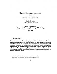
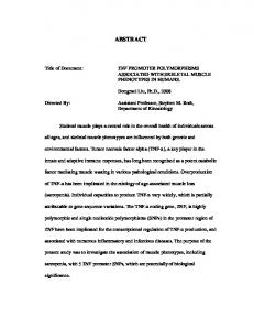
3 Evaluating the Integral We shall apply the divide-and-conquer strategy for integral evaluation. When there are several vertices of the polygon inside the mask, we may break the integral region into several components by linking the pixel center and the vertices (Figure 2). When there is no vertex inside the circle (Figure 3(a)), the region is not further broken. If the pixel center is on the left of the polygon edge, the corresponding component integral, or the integral over the component region, is added to the accumulation buffer. Otherwise the negative component integral is added (Figure 2(b)). After the traveling is finished, the accumulation buffer is not exactly the desired integral. Instead, it can be either negative or larger than 1, but the difference from the exact value is always an integer (Figure 2(b)). We have not found a convenient way to resolve such difference. Nevertheless, as long as we are sure that the exact value must be between 0 and 1, we may shift the accumulation buffer by integers to make it between 0 and 1. Then the accumulation buffer must be identical to the exact value. The price paid for this compromise is that only non-negative filters can be used in SplitRender. Otherwise, our system cannot judge whether a buffer should be shifted if its value is negative or larger than 1. Now the problem becomes how the component integrals are computed. It can be seen that there are three kinds of component regions (Figure 3), depending on how many ends of a polygon edge are inside the filter mask. Note that the first kind is a special case of the second when the vertex is on the boundary of the mask, and the third is the difference between regions of the second type (Figure 3(d)). Consequently, an integral can be computed by combining only one type of basic component regions, shown in Figure 3(b). By defining a new coordinate (Figure 4(a)), where the t-axis is along the marching direction of the polygon edge and the d-direction is π/2 behind the t-direction, the basic component region can be parameterized by the coordinate of the polygon vertex V in the new coordinate, i.e., the distance d from the pixel center to the polygon edge and the distance t between the vertex V and the projection of the center onto the
2
=
+
+
(a) = (−
) + (−
) + (−
)+1
(b) Figure 2: The integral region is split into component regions by linking the pixel center and polygon vertices. (a) If the pixel center is on the left of the polygon edge, the component integral is added to the accumulation buffer. (b) Otherwise, the negative component integral is added. There is integer difference between the final accumulation buffer and the exact value.
= (a)
(b)
(c)
− (d)
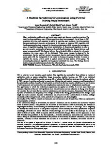
Figure 3: The component regions. (a)∼(c) Three kinds of component regions, where the polygon edge has 0, 1 or 2 ends inside the filter mask, respectively. (d) Further decomposition of the region in (c). polygon edge. When non-circular filters are used, an extra parameter θ, which is related to the polar sweep angle of the d-axis (Figure 4(b)), is also necessary for the parameterization. If the vertex coincides with the pixel center, the basic component region is not well defined. However, this ambiguity can be conveniently solved by adding a tiny displacement (1/512, 1/512) to the vertex so that the parameters can be computed appropriately. At the same time, the difference from the exact integral is less than 1/256 and the integer pixel values will not change. A look-up table can be built for the basic component regions. Then the integral over the part of a polygon inside the filter mask can be computed by combining the basic component regions and then looking up the table. However, fine anti-aliasing usually requires a large look-up table. Otherwise, random noise due to quantization may appear (Figures 7(c)(e)(f) and 8(c)(e)(f)). This calls for long preparation time of the look-up table and large memory, especially when the table is 3D. To remedy this problem, we use low-order polynomial filters, either circular or square, that can provide closed-form solutions for the integral over basic component regions and achieve excellent anti-aliasing results. Please refer to [6] for more detail.
4 Experimental Results We first present the pre-filtering results of SplitRender using various filters 1 . The test patterns, a wheel and a checkerboard, are shown in Figure 5. There are 180 triangles in Figure 5(a), while Figure 5(b) has 92,100 quadrilaterals, most of which are extremely small and are at the top of the image. Figure 5 is rendered by SplitRender using our square polynomial filter with radius 2 [6]. We see that the rendering results are almost aliasing-free. The filters used are all of radius 2, including our square polynomial filter, our circular polynomial filter [6], box filter, and circular Gaussian filter with σ = 0.9. We choose the box filter and the Gaussian filter because they are very common in computer graphics. For the box filter and our circular polynomial filter, both analytic evaluation and look-up tables are applied. For the circular Gaussian filter, σ is chosen as 0.9 by visual comparison so that the rendered results have optimal balance between eliminating the aliasing and keeping the image sharp. When a filter uses a look-up table, the size of the table is always 129 × 257 (i.e., d and t are uniformly divided into 128 and 256 parts, respectively), and nearest-neighbor interpolation is used if (d, t) is not a sample point. We do not provide higher-resolution look-up tables 1 The
full-resolution images for Figures 5∼9 are available online at http://www.acm.org/jgt/papers/LinEtAl04.
3
y
y R
R V
d
d
t
t
V
R
O
R
O
x
(a)
x
(b)
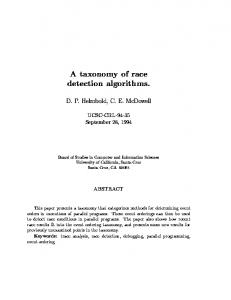
Figure 4: The basic component region (shaded area) is bounded by one polygon edge, one radius passing the polygon vertex and the filter boundary. (a) For circular filters, the parameterization (d, t) is 2D. (b) For square filters, the parameterization (θ, d, t) is 3D. because we want to exemplify that using look-up tables can result in random noise when the details are beyond their resolutions and on the other hand larger look-up tables require too much storage. We do not use the square Gaussian filter and do not apply a look-up table to our square polynomial filter because the required look-up tables are both 3D, demanding huge storage. Figures 6∼8 show the zoom-ins of the rendered results using various filters. Our polynomial filters (Figures 6(a)(b)(c), 7(a)(b)(c), 8(a)(b)(c)) are better than the box filter and the Gaussian filter (Figures 6(d)(e)(f), 7(d)(e)(f)), 8(d)(e)(f)). When look-up tables are used, random noise is unavoidable at places that have fine details. For example, the random noise near the bottom-left of Figures 6(c)(e)(f) is perceptible because the triangles swarm there, while the noise become apparent at the top of Figures 7(c)(e)(f), 8(c)(e)(f) because the quadrilaterals are extremely small. In contrast, when analytic evaluation is applied, the random noise is completely removed (Figures 6(a)(b)(d), 7(a)(b)(d), 8(a)(b)(d)). For comparison, we also render the patterns in Figure 5 by uniform super-sampling. The filter used is the MitchellNetravali filter [7] with B = 1/3 and C = 1/3. It is of size 2 by 2. This family of filters have been reported to have good anti-aliasing performance [7, 5, 3]. The sampling rate is 1024 (32×32) points per pixel. We deem that 1024 is a high enough sampling rate because we have not seen any example in the literature with a sampling rate higher than 256. Though the results with the Mitchell-Netravali filter (Figures 9(a)∼(c)) look sharper, the aliasing is also more visible than that rendered by our polynomial filters. Moreover, the random noise is still visible (top of Figures 9(b)(c)) even at such a high sampling rate. This is due to an insufficient sampling rate for pixels containing tiny quadrilaterals. The above examples testify that pre-filtering with closed-form evaluation is more suitable for high-quality antialiasing. Using look-up tables or super-sampling always introduces random noise if the size of graphical objects is beyond their precision.
5 Discussion A main disadvantage of SplitRender is that it does not support filters with negative lobes. However, we exemplify in [6] that choosing appropriate non-negative filters, such as our optimal polynomial filters, suffices to achieve high-quality anti-aliasing results. Another defect is that SplitRender is hard to be fully hardware accelerated. Currently we only optimize it by fixedpoint computation and output to screen via DirectDraw. To render Figure 5(a) on our Pentium IV 1.3GHz PC, it takes about 80 milliseconds using analytic evaluation with the square polynomial filter of radius 2 and about 5 milliseconds using a 129 × 257 look-up table computed from the circular polynomial filter of radius 2. We are still seeking more hardware acceleration. In principle, SplitRender can support graphical objects with piece-wise polynomial textures (just raise the orders of polynomials in the formulae of the component integral, see [6]), though we have not implemented so. We are also investigating the pre-filtering of more generally textured graphical objects.
4
(a)
(b)
Figure 5: The rendering results of SplitRender using the square polynomial filter with radius 2, closed-form solution used.
References [1] B. Ackland and N. Weste. Real time animation playback on a frame store display system. In SIGGRAPH 1980 Conference Proceedings, Annual Conference Series, pages 182–188, July 1980. [2] Tom Duff. Polygon scan conversion by exact convolution. Raster Imaging and Digital Typography ’89, pages 154–168, 1989. [3] A. E. Fabris and A. R. Forrest. Antialiasing of curves by discrete pre-filtering. In SIGGRAPH 1997 Conference Proceedings, Annual Conference Series, pages 317–323, August 1997. [4] E. A. Feibush, M. Levoy, and R. L. Cook. Synthetic texturing using digital filters. In SIGGRAPH 1980 Conference Proceedings, Annual Conference Series, pages 294–301, July 1980. [5] Brain Guenter and Jack Tumblin. Quadrature prefiltering for high quality antialiasing. ACM Trans. on Graphics, 15(4):332–353, 1996. [6] Zhouchen Lin, Hai-Tao Chen, Heung-Yeung Shum, and Jian Wang. Optimal polynomial filters. Journal of Graphics Tools, ??(??):??, 2004. [7] Don P. Mitchell and Arun N. Netravali. Reconstruction filters in computer graphics. In SIGGRAPH 1988 Conference Proceedings, Annual Conference Series, pages 221–227, August 1988.
5
(a)
(b)
(c)
(d)
(e)
(f)
Figure 6: Zoom-in of the polygons in Figure 5(a) rendered by SplitRender using filters with radius 2. (a) Square polynomial filter, closed-form solution used. (b) Circular polynomial filter, closed-form solution used. (c) Circular polynomial filter, look-up table used. (d) Box filter, closed-form solution used. (e) Box filter, look-up table used. (f) Circular Gaussian filter with σ = 0.9, look-up table used.
6
(a)
(b)
(c)
(d)
(e)
(f)
Figure 7: A zoom-in of the polygons in Figure 5(b) rendered by SplitRender using filters with radius 2. (a) Square polynomial filter, closed-form solution used. (b) Circular polynomial filter, closed-form solution used. (c) Circular polynomial filter, look-up table used. (d) Box filter, closed-form solution used. (e) Box filter, look-up table used. (f) Circular Gaussian filter with σ = 0.9, look-up table used.
7
(a)
(b)
(c)
(d)
(e)
(f)
Figure 8: Another zoom-in of the polygons in Figure 5(b) rendered by SplitRender using filters with radius 2. (a) Square polynomial filter, closed-form solution used. (b) Circular polynomial filter, closed-form solution used. (c) Circular polynomial filter, look-up table used. (d) Box filter, closed-form solution used. (e) Box filter, look-up table used. (f) Circular Gaussian filter with σ = 0.9, look-up table used.
(a)
(b)
(c)
Figure 9: Zoom-in of the polygons in Figure 5 rendered by uniform super-sampling at 1024 points per pixel. The filter used is the Mitchell-Netravali filter [7] with B = 1/3 and C = 1/3.
8