Apr 15, 2017 - ation from two different standpoints i)a single ray emanating from a source. 1. arXiv:1704.04668v1 [physics.geo-ph] 15 Apr 2017 ...
arXiv:1704.04668v1 [physics.geo-ph] 15 Apr 2017
Pre-stack deconvolution revisited Jagmeet Singh Regional Computer Centre, ONGC Ltd, Vadodara,India
April 18, 2017
Abstract While in the case of zero offset data with horizontal beds, it is clear that the recorded trace is a convolution of the wavelet and reflectivity series, the situation in the case of finite offset is a bit more complex as the direction of the incident ray is not vertical, the natural direction in which the reflectivity series is measured.We examine the consequences of this hitherto neglected fact.
Introduction While in the case of zero offset data with horizontal beds, it is clear that the recorded trace is a convolution—say w1 R3 + w2 R2 + w3 R1 — of the reflectivity encountered along the incident vertical ray and the wavelet [1], the situation in the case of finite offset is not so simple. For finite offset, the direction of the incident ray is not vertical, the direction along which one would normally measure the reflectivity series.A question that arises naturally is:- ’what is the direction along which time/reflectivity series is measured-is it the slant direction along the incident ray or the vertical direction?’.We examine this question as well the consequences of two directions involved below.Origin of time is clearly the moment of initiation of blast. In the section below namely Different Ray Paths , we examine the situation from two different standpoints i )a single ray emanating from a source 1
hitting different reflectors at different CMP’s and ii ) multiple rays maintaining the same CMP. We restrict ourselves to the case of horizontal reflectors in this paper.We shall examine whether the idea of convolution survives or not– whether we have to think in terms of convolution or consider the recorded amplitude at a particular time as just an ’amalgam’ of amplitudes reflected from nearby reflectors).In the next section, we take a critical look at the idea of predictive deconvolution in the case of finite (non-zero) offset.A section looking critically at the idea of τ -p deconvolution then follows.Finally, we draw main ideas of the paper in the last section Conclusions.
Different ray paths As discussed above, a slant incident ray meets the series of reflection coefficients in the slant direction, whereas the series itself is defined in the vertical direction. Figure 1 shows a single ray path that meets different reflection coefficients R1 ,R2 and R3 at different times along the slant path.When we write h(t) = w(t) * R(t),what is the origin of time the for the three quantities involved? Obviously,all the three quantities must refer to the same origin of time —the moment the source S blasts. Even the reflectivity series has to bo measured/sampled along the slant direction i.e. the ray direction. If one assumes that the reflectivity series is the series of reflection coefficients measured in the vertical direction, the convolution won’t stand. In figure 1 , the difference in times between w1 and w2 (in the convolution sum w1 R3 + w2 R2 + w3 R1 ) must match the difference in times between R3 and R2 which happens when time axis for w and R is the same. If we insist on defining reflectivity in the vertical direction independent of the direction of the incident ray,the resulting ’convolution’ would be something like Z ∞ h(t) = w(τ )R((t − τ ) sin θ)dτ (1) −∞
where θ is the angle between the incident ray and the horizontal.This is clearly not a convolution as long as sin θ sits in the equation(only when θ is 90◦ i.e. the case of vertical incidence, true convolution is restored).A simple solution then is to redefine refectivity series as the one sampled along the slant direction of the incident ray itself rather than the vertical direction.However, as shown in Figure 1 below, we find that the reflections ( w1 R3 , w2 R2 , w3 R1 )that would normally be received at a single receiver (in 2
Figure 1: A single ray path getting reflected and received at multiple receivers the case of zero offset), are received at different receivers. So, the reflected amplitudes that were supposed to exist in the convolution sum at a single location are in fact being received at different receivers. A possible solution to restore the convolution could be to simply add across the traces at R1,R2 and R3 i.e. a kind of local stack.But why generate a convolution when it’s not there in the first place. Let us now look at the picture from another angle. Instead of looking at a single incident ray, let us examine what is received at a single receiver from a source (Figure 2). The source S is reflected at the three reflectors shown to produce virtual sources S”’,S’ and S’. Three ray-paths result corresponding to different depths but the same CMP. Can such a trace be looked upon as a convolution between the wavelet and the reflection coefficients ? The important difference here is that there are multiple ray paths involved. In the case above, reflectivity series is measured along a single ray, whereas, here, it is 3
Figure 2: Multiple ray paths getting reflected and received at a single receiver being measured along different rays.It is indeed a problem that there is no single direction along which reflectivity is measured.However,whatever may be the awkward direction-changing sequence of reflection coefficients,we may still call it as a ’convolution’ between the wavelet and the reflection field(field of reflection coefficients) as measured from the source point.Since time differences between two oblique rays in Figure 2(which is different from the time differences between corresponding vertical rays) must match time differences between the wavelets at the two locations, there would be a diiferent set of terms in the convolution sum.That is the degree of convolution in the slant case would be different from the one in the vertical case.For a single trace recorded at a receiver, the angle changes with depth and the terms participating in the convolution also change i.e. shallow reflectors may be more convolved than the deeper ones.As we go deeper and deeper, we go closer to the vertical case.
4
To quantify the two dimensional nature of the problem(case of slant rays), note that the argument of the wavelet is actually (t − r/c) i .e. the wavelet should be written as w(t − r/c)(instead of simply w(t)) where r = |~r| is the distance travelled from the source point to the reflector and c is the wave speed. We define a hypothetical trace h(t), summing over all amplitudes received at the surface from different reflection points ~r at two way time t as Z h(t) =
w(t − r/c)R(~r/c)d(~r/c),
(2)
where we have used argument of reflection coefficient as ~rc instead of ~r to let arguments of both w and R be in time.By d(~r/c), we mean rdrdθ/c2 and R(~r/c) means R(x/c, z/c). Why we call it hypotheical is because it is never recorded as it sums over all possible positions ~r–if the x component of ~r is not fixed, the reflections are received at different receivers. So, in the above equation we need to integrate over z keeping x fixed if we need to find the amplitude received at one receiver i.e. p Z (x2 + z 2 ) x z h(t, x) = w(t − )R( , )dz/c. (3) c c c For the flat reflector case that we are considering, dependence of R on x in the above equation may be dropped.Clearly equation (3) does not represent a convolution.So, what’s wrong? The answer is nothing–the recorded trace is not a convolution between the reflectivity measured in the vertical direction and the wavelet!There is, however, another way of looking at the problem – the reflector is met when t=r/c and the reflectivity is referred to time t with the origin of time as the moment of initiation of the blast.With reflectivity series defined in two way time r/c, equation((2)), for the case of constant x(single receiver) may be re-written as
Z h(t, x) =
p p (x2 + z 2 ) (x2 + z 2 ) z w(t − )R( , x) p dz, 2 c c c (x + z 2 )
(4)
p where we have written arguments of R as the two way time (x2 + z 2 ) as well as position x.We need an additional qualifier x because same 5
time( used
p 2 (x + z 2 )/c) may correspond to two different x(or z).Further,we have zdz d(r/c) = p , c (x2 + z 2 )
valid for the case of constant x.Defining p (x2 + z 2 ) τ= , c we see that the above may be re-written as: Z h(t, x) = w(t − τ )R(τ, x)dτ,
(5)
which looks like a convolution at least for a constant x.The reflectivity series is sampled differently at different x, so that we need an additional qualifier x in R, even for the case of horizontal reflectors.So, is the convolution restored(for a constant x)?Another question that arises is ’which equation ( (3) or (4)) describes correctly the amplitude recorded at x?’.Both equations (3) and (4) need a slight modification–both have dimensions of time and need to be normalised.We need to divide (3) by two way vertical time t0 corresponding to time t = R/c (where R is the distance upto reflector met by wavelet amplitude w0 ) i.e. t = Z/c, and (4) by two way time t.When we do this, it’s easy to see that equations (3) and (4)are essentially the same–they are two ways of looking at the same problem.And yes, for a constant x(and flat reflectors), we can say the trace is a convolution of the wavelet and reflectivity measured in two way time. √ Note that although the limits of integration are from z = 0 to z = c2 t2 − x2 , the lower limit is much higher than zero because the wavelet is of a limited duration say τ .So lower limit of z is set by the equation p (x2 + z 2 ) t− =τ c
(6)
Regarding the change of degree of convolution with depth in a trace, we need to look back at the relation zdz d(r/c) = p c (x2 + z 2 ) 6
or
dz d(r/c) = p c (1 + x2 /z 2 )
We see that as we go deeper i.e. z increases, we get closer to the vertical difference dz/c and at shallower z, the difference is lower than dz/c meaning thereby more terms in the convolution.That is, shallower reflectors are more convolved than the deeper ones in a finite offset trace.Though with equation (5), we have managed to give our amalgam of amplitudes, mathematically, the shape of a convolution–we have to understand the limitations of such a definition.With time varying degree of convolution in a trace represented by equations (4),(5) and with different reflectivity series across a gather(although R is not a function of x), deconvolution would be problematic.For example,in the case of surface consistent deconvolution,we expect a single deconvolution operator for a shot gather(other things being equal i.e. identical receivers in identical surface conditions)–this is clearly not right.Also even for a single trace deconvolution,we expect the whiteness of the reflectivity series to be disturbed by the irregular sampling of the reflection series by slant rays–reflectivity series would be denser at shallow times and sparser as we go deeper. One may be tempted to think that NMO which maps two way slant time t onto two way vertical time t0 would solve the problem i.e. restore the 1D convolution suggesting NMO befere deconvolution. But the constituents of the amalgam remain the same–it’s just that the amalgam h(t) is mapped onto h(t0 ) This will not be the same as 1D convolution recorded in the case of zero offset. What we arrived at intuitively in the two cases described above is very well encapsulated in the equation above.The equation (3) corresponds perfectly to the case 2 (Figure 2) discussed above.To cover case 1, we need to fix the angle θ in equation(1) so that we get Z h(t, θ) = w(t − r/c)R(r, θ)d(r/c), (7) where we have dropped the integration over θ.Note that this sum of amplitudes is also not recorded as its constituents are received on different receivers. We also need to consider the Fresnel zone at the surface in case 1.If the constituents of the amalgam of amplitudes reaching different surface locations fall within the Fresnel zone, we may as well take them to be recorded by a single receiver. However, for the sake of simplicity, we shall 7
assume here the Fresnel zone to be small enough and receivers well separated so as not to consider this case.
Predictive deconvolution All predictive deconvolution algorithms available in the seismic industry assume the simple 1D convolution h(t) = w(t) ∗ R(t). Now that we agree that what is recorded at a single receiver R is some amalgam of amplitudes arising from reflections from different rays or a convolution in limited sense, the next questdon that arises is ‘can we retain an idea similar to predictive deconvolution?’. Obviously, for predictive deconvolution to work, we need predictability apart from a convolution (which is true in a limited sense).We examine predictability here & we shall restrict ourselves to the case of horizontal reflectors. Predictability of the wavelet generally comes from a source of reverberation like the sea surface. Imagine sea surface lying just above source S and receiver R shown in Figure 3 and the first reflector being the water bottom.We see that the periods of the multiple energy corresponding to different rays shown are different and also received at different receivers, so we focus instead on multiple energy received at a particular receiver.We see that multiples received at a particular receiver would be generated from different CDP’s(whereas primary energy is from the same CMP (for the caseof horizontal reflectors) and the periods of multiple from different reflectors would be different. Cleadly, predictive deconvolution in the pre-stack case as a multiple attenuator fails. Even if we consider a single trace as a convolution of the wavelet and reflectivity series , the period of multiples is not fixed and predictive deconvolutnon as a multiple attenuator will not work. So, what is the way out?In Figure 4 , we show rays with same angle recorded at different receivers at different times.Such energy would be difficult to isolate, but would be convolutional.However, multiple energy corresponding to these primaries would be received at different receivers–so we have to reject this idea. We mentioned possible summation across traces while discussing the case of single ray—this reminds one of the slant stack[1]. A plane wave is received by multiple receivers— is the stack along the plane ( of the plane wave) a convolution? A beauty about the plane wave is that the period of the mutiple is fixed for a particularly directed plane wave i.e. a plane wave with 8
Figure 3: Multiple generation from sea surface
9
Figure 4: Rays with same angle
10
a particular p value. So, in this case, does predictive deconvolution work?We examine this question in the next section. Slant Stack Relooked An array of sources with suitable delays is expected to generate a plane wave. Since we have a single source in a shot gather, we simulate a plane wave by introducing the delays in the array of receivers instead. What is however recorded by the receivers is not pure plane waves as they have been altered by the reflectors.A more rigorous interpretation of the case in hand is that of a point source(time harmonic) which is a summation of plane waves via the Sommerfeld-Weyl integral [2].A real wavelet of finite duration is, of course, however simulated by a superposition of such time harmonic point sources.We assume that the modification of these plane waves by the reflectors is such that the sum over delayed receivers at a given p yields a convolution sum of these plane waves with the reflectors or in other words a convolution of the wavelet and the reflectors in zero offset time, so that a subsequent deconvolution in the τ − p domain would be justified.However, as the angle of incidence increases, the reflected plane waves are recorded by less and less of the spread of receivers–so this is a limitation that we need to keep in mind.Moreover, even in the case of infinite spread, we need to see mathematically if the slant stack is really a convolution of the wavelet and reflectivity in zero offset time or not. We work it out below.Starting with the definition of trace at a particular x Z h(t, x) = W (t − t0 )R(t0 , x)dt0 , (8) √ where t0 = x, we get
(x2 +z 2 .Making c
the substitution t = τ + px, and summing over Z
H(p, τ ) =
W (τ + px − t0 )R(t0 , x)dt0 dx,
(9)
Introducing Z W (t) =
W (ω) exp(ιωτ )dτ,
we write equation (9) as Z H(p, τ ) = W (ω) exp(ιωτ ) exp(ιω(px − t0 ))R(t0 , x)dωdxdt0 ,
(10)
(11)
we get Z H(p, τ ) =
W (ω) exp(ιω(τ + px)R(ω, x)dxdω, 11
(12)
where we have used the identity Z R(ω) = R(t0 ) exp(−ιωt0 )dt0
(13)
Note that factors of 2π etc. have been left out as these would cancel out in the use of inverse and forward transforms given by equations (10) and (13).Equation (12) wonderfully describes τ − p transform as a sum of plane waves with amplitudes as a product of R(ω,0 x0 ) and W (ω)–this is meaningful only when dependence of R on x can be dropped.With a little re-arrangement, we can show that H(τ, k) = W (τ ) ∗ R(τ, k)
(14)
H(τ, x) = W (τ ) ∗ R(τ, x),
(15)
or so it is H(τ, x) or H(τ, k) rather than H(τ, p), which is the desired convolution– i.e. convolution of the wavelet and reflectivity in zero offset time τ .So, in our view τ − k deconvolution instead of τ − p deconvolution is more meaningful.However, note that, in arriving at the last two equations, sign convention used for Fourier transform of x and t is not the same.
Conclusions Although there is nothing wrong with deconvolution of a zero offset trace,one needs to be careful while extending the idea to the p case of non-zero offset.Reflection coefficient series R(t0 ) is mapped onto R( (t20 + x2 /v 2 )) whereby it becomes a function of both time and offset.Gather level deconvolution i.e. a single deconvolution operator for a gather is not meaningful.Predictive deconvolution as a multiple attenuator is also not meaningful.Trace level spiking deconvolution may be tried to compress the wavelet/recover the reflectvity series.However, the assumption of whiteness of reflectivity series is not quite true in this case.We have also examined the slant stack critically, and found that if deconvolution is to be attempted in this domain,τ − k or τ − x deconvolution rather than τ − p deconvolution is more meaningful.
12
References [1] O. Yilmaz. Seismic Data Analysis, 2nd edition. Society of Exploration Geophysicists, 2001. [2] M. Tygel and P. Hubral. Transient representation of the SommerfeldWeyl integral with application to the point source response from a planar acoustic interface. Geophysics, 49(09):1495–1505, 1984.
13