Precise Image Segmentation for Forest Inventory - Robotics Institute

Precise Image Segmentation for Forest Inventory Jeffrey Byrne and Sanjiv Singh CMU-RI-TR-98-14

The Robotics Institute Carnegie Mellon University 5000 Forbes Avenue Pittsburgh, PA 15213 May 1998

© 1998 Carnegie Mellon University

ii

Abstract This paper presents a portable vision system for forest surveying that can estimate the diameter of a target tree with a single “point and click”. Of specific interest is the texture segmentation algorithm used for accurately determining the boundaries of the target tree in a forest. This segmentation is challenging because the target may be occluding other, almost identical looking trees, creating an obscure edge. To compensate for this possibility, we have created an algorithm sensitive to small texture changes which uses both the co-occurrence matrix and the Mahalanobis metric to first find a window that must contain the target texture edge. Then, the edge is precisely localized in this window using a novel method based on co-occurrence matrix differences. Using this algorithm, given no structured shadows, we have been able to achieve consistent accuracies of +/- 1 inch, or less than 5% error, in both simulated tests and a field trial.

iii

iv

Table of Contents 1.0 Introduction ......................................................................................................................1 1.1 Research Problem .................................................................................................. 1 1.2 Summary ................................................................................................................ 3 2.0 Image Segmentation .........................................................................................................4 2.1 Related Work ..........................................................................................................5 2.1.1 Texture Measurement ..............................................................................6 2.1.2 The Co-occurrence Matrix ......................................................................7 2.1.3 Texture Comparison ................................................................................8 2.1.4 The Mahalanobis Metric ......................................................................... 9 2.2 Texture Segmentation Algorithm .........................................................................10 2.2.1 Preprocessing - Gray Level Reduction ................................................. 11 2.2.2 Training .................................................................................................11 2.2.3 Mahalanobis Difference Computation ..................................................12 2.2.4 Adaptive Mahalanobis Difference Computation ...................................13 2.2.5 Edge Localization ................................................................................. 14 2.2.6 Edge Finding by Linear Regression ......................................................16 2.2.7 Complete Segmentation ........................................................................ 16 3.0 System Design .................................................................................................................18 3.1 Design Criteria ...................................................................................................... 18 3.2 Related Work ........................................................................................................18 3.3 Candidate Solutions ............................................................................................ 19 3.3.1 Scanning Laser Rangefinder ................................................................. 19 3.3.2 Spot Laser Rangefinder .........................................................................19 3.3.3 Full Frame Stereo ..................................................................................19 3.3.4 Line Scan Stereo ................................................................................... 19 3.3.5 Laser/Camera Hybrid ............................................................................20 3.4 Comparison of Candidate Designs .......................................................................20 3.5 Proposed Solution ................................................................................................ 20 4.0 Results ............................................................................................................................. 22 4.1 Simulated Environments ...................................................................................... 22 4.1.1 Radically Different Backgrounds ..........................................................22 4.1.2 Occlusions .............................................................................................23 4.1.3 Shadows ................................................................................................ 24 4.2 Field Results .........................................................................................................25 5.0 Conclusions .....................................................................................................................28 6.0 References ....................................................................................................................... 30

v

vi

1. Introduction Product inventory is an especially hard problem in commercial forestry. Deciding if a new piece of forest is worth buying, or measuring the growth on currently owned land requires special inventories called survey runs. The ultimate goal of a survey run is to determine the total harvestable wood volume in a survey area. To do this, a surveyor must first measure the height and diameter at approximately chest level of a sample set of trees in the survey area. Subsequent analysis then extrapolates this data to represent the total harvestable wood volume. Currently, tree diameter and height measurements are made by trained surveyors relying only on experience and simple optical devices. Estimates from experts suggest that due to the subjective nature of these methods, inventory on a per-area basis can vary up to 25% from the true value. While some commercially available instruments now provide better height estimation accuracy than conventional methods, diameter estimation using such instruments remains relatively slow and difficult to use. Automating this task offers the potential of improving accuracy, providing real time data logging and analysis, growth-rate feedback early in the product cycle, and reducing labor. In this report, we describe the design and testing of a system created to automate the process of diameter estimation.

1.1. The Research Problem Diameter estimation is largely a problem of image segmentation. As shown in Figure 1, assuming a cylindrical model, diameter (D) can be estimated from the range to target (R) and the angle subtended by the target or angular size (α).

D

Cylinder Cross Section R

α

Sensor

α 2R( sin ---) 2 D = ----------------------α 1 – sin --2 Equation 1

Figure 1: Diameter estimation parameters

Range measurement is a well understood problem and can be done using conventional methods such as lasers or various image processing techniques. Angular size measurement, however, is not as straightforward since the exact location of the target in a scene must be known. This location can be found by segmenting an image of the scene into target and background. 1

Depending on the sensor used, segmentation can be performed on either range or reflectance images. Range sensors are attractive since it is relatively straightforward to determine shape directly from sensed data and segmentation is generally easier. However, range sensors require moving parts and can be expensive. In contrast, segmentation of reflectance images, though computationally more challenging, holds the promise of a low cost system with no moving parts. For these reasons we propose to base the angular size measurement on reflectance image segmentation. Image segmentation of natural scenes is complicated by several issues. First, lighting cannot be easily controlled. Shadows cast by objects blocking ambient light are common and can potentially obscure the target edge. Second, objects in nature are rarely planar. Variations in shape can change the look of the target, making segmentation more difficult. Third, partial occlusions can obscure the edge boundary. This is true for a general outdoor scene, but it is especially true for what can be described as an homogeneous scene. An homogeneous scene contains many almost identical objects at various locations. A partial occlusion in such a scene makes the edge finding especially difficult since the occluded object and the target look quite similar (Figure 2c). Segmentation must be sensitive to such boundaries as well as obvious boundaries as in the more typical case shown in Figure 2b.

Figure 2: Tree image segmentation. (a) Raw image (b) Simple segmentation (c) Close up of segmentation in case of partial occlusion of a tree behind the target tree

Therefore, the research problem present in non-contact diameter estimation is creating a robust image segmentation algorithm that will find the correct target edge even in the presence of shadows, non-planarity and very similar looking occlusions. In addition, diameter estimation accuracy is directly dependent on how accurately the target edges are found, so this algorithm must also accurately localize the target edge boundary.

2

1.2. Summary This report describes the design and testing of a system to perform non-contact diameter estimation, focusing on the computer vision algorithm created to handle the outdoor segmentation issues present in a forest scene. Chapter 2 describes this algorithm in detail along with background on similar segmentation systems and research done in image segmentation using texture. Chapter 3 describes the design of a system used to perform this task. Five possible solutions are explored, and from these, it is shown that a spot laser boresighted with a camera best meets the design goals. Chapter 4 shows that in both simulated environments and an actual survey run, this system can achieve high accuracies. Finally, Chapter 5 gives conclusions about overall performance and recommendations for improvements.

3

2. Image Segmentation As shown in Figure 1, diameter estimation requires range to target (R) and angular size ( α). Section 1.1 argues that the most cost effective method of measuring angular size is by accurately segmenting a reflectance image into target and background. However, this segmentation is not trivial since a target tree is non-planar, and is quite similar looking to other trees nearby. This chapter will focus on the computer vision algorithm created to perform this segmentation. Good image segmentation relies on extracting the most significant differences between image regions, and in most natural settings, these significant differences are color and texture. In a forest, texture may be a better segmentation basis since color is fairly constant from tree to tree of the same species while texture changes significantly. In general, image textures can be broken into three categories, periodic, nearly periodic or random [5]. Periodic textures, such as a crystalline lattice from electron microscopy, have a regular, completely deterministic pattern. Nearly periodic textures, such as the stitches in a sweater, are close to being periodic, but have added noise. Random textures, such as pebbles on a beach, have regularity only in a statistical sense. Most commonly occurring natural textures, including tree bark, are random. An algorithm that will segment target tree texture from background texture must be sensitive to random texture, must not be confused by a non-planar surface, and must accurately localize the texture boundary even when this boundary is obscured, given an occluded tree as in Figure 2c. Many researchers have created general algorithms for texture segmentation, including such methods as active contours or snakes, Bayesian inference and region growing. These algorithms work well, but most are created to be used on planar textures [9][13], such as those found in the Brodatz set. Also, many algorithms that can reliably locate regions of differing texture do not always accurately localize texture boundaries, especially when presented with an obscured edge [6][12][14]. Therefore, a new algorithm must be created that can compensate for a non planar surface, find texture boundaries accurately even when presented with an obscured edge, and be optimized for use in a forest setting. To create this algorithm, similar outdoor segmentation systems are first explored to gain insight into the problem. This is followed by a discussion on current research in texture segmentation to find methods best suited to this application.

4

2.1. Related Work Many researchers have successfully created outdoor vision systems. One interesting system developed by Ollis and Stentz navigated an industrial alfalfa harvester by following the cut/uncut crop line in a field. To do this, a color image was taken of a field, and a best fit step function was computed for each image scan line using the fisher linear discriminant in RGB space [11]. Figure 3 shows the results obtained in a field using this method as well as the line found between compacted and uncompacted garbage using texture as a discriminant instead of color. This problem is surprisingly similar to the forest segmentation problem since both break an image into two regions, (cut/uncut vs. tree/background), and both segment along roughly vertical boundaries. However, this method uses a best fit step function which assumes that the region boundary is always clear, and in a forest an occluded tree many obscure the edge. Even though this algorithm is not directly applicable, this system does add insight to the design of robust outdoor vision systems. Most importantly, Ollis and Stentz found it necessary to perform a shadow removal step in order to compensate for ambient lighting changes. This problem is present with many outdoor vision systems and may influence results in a forest.

Figure 3: Segmentation using (a) color for finding the edge of cut crop (b) texture for finding the line between compacted and uncompacted garbage. The white line shows the result of the segmentation algorithm. Results due to Mark Ollis

Researchers have also done work to develop methods of image segmentation using texture. In general, texture segmentation algorithms must first measure texture in a region then compare this texture to the texture in other regions to test for similarity. Both texture measurement and texture comparison methods will be explored in the next section to find a method best suited for use in 5

this application. 2.1.1. Texture Measurement In general, texture measurement can be broken into five categories: spectral, multiscale, model based, structural and statistical methods [10]. Spectral methods such as the short-term fourier transform (STFT) or 2D power spectrum analysis measure the localized frequency content of an image. This method is particularly well suited, and is typically used for, the segmentation of images containing planar, periodic textures [9]. Since most naturally occurring natural textures are random and not periodic, this method may not be the best choice. Multiscale methods, such as wavelet analysis, also measure the localized frequency content of a signal, but, to achieve optimum space/frequency resolution, the window function varies with frequency instead of remaining a constant size. Again, this method is typically used for the segmentation of periodic or nearly periodic textures. Rubner and Tomasi have successfully applied this method to random textures [12], but their method unfortunately discards boundary areas as containing insufficient texture for segmentation. Since boundary areas are the ultimate goal of this segmentation, this method is again not the best candidate. Model based methods, such as Markov random fields, use many samples of a texture to create a general statistical model, where segmentation is done by checking how well new textures fit the model. This method has been successfully used in the segmentation of natural scenes, but common problems with this approach are the time and number of texture samples required for model creation [13]. This method is a possible choice since it has been proven to work with natural textures, however, the complexity and speed of the computation must be taken into account as negative factors. Structural methods, such as the texton model proposed by Voorhees and Poggio [13], extract texture primitives or macrotextures, such as blobs of similar color or shape, from an image. The density and other first order properties like width or length may then be used to group similar looking regions. This method and has been successfully applied to the segmentation of naturally occurring textures, and is a candidate for use here. Finally, statistical methods, such as the co-occurrence matrix proposed by Haralick et al. [4], extract microtextures such as local gray levels pairs to determine the texture of a region. This method has been widely used and can be applied to random textures. Therefore, it would seem

6

that the most promising methods of texture segmentation for this problem are structural methods and statistical methods, both of which have been successfully applied to naturally occurring random textures. The co-occurrence matrix, a statistical method, was chosen because it is an intuitive measure of texture, and is straightforward to compute. 2.1.2. The Co-occurrence Matrix The co-occurrence matrix can be described as "a matrix conveniently representing the occurrences of pairs of gray levels of pixels, that are separated by a certain distance and lie in a certain direction (angle) in an image." [4] Given an image I with m different gray levels, two pixels, i1 and i2 in I can be represented by: i1 = I(x1, y1)

i2 = I(x2, y2)

where x is the row location, y is the column location, and i is the gray value of the pixel. Let d be the distance that separates these two pixels, where d = 1 means neighboring pixels, and d = 2 means pixels separated by one pixel and so forth. Finally, let θ be the angle along which the pairs of pixels lie, typically 0, 45, 90, and 135 degrees. The co-occurrence matrix is an mxm square matrix. Suppose ik and ij are two gray values separated by a distance d along the angle θ in the original image. Also suppose that these gray values occur in this configuration of d and θ N times in the image I. The co-occurrence matrix is therefore the mxm matrix such that Pθ d (i k,i j) = N

Co-occurrence entries exist for each combination of gray value in the image, and a new co-occurrence matrix exists for each different choice of d and θ. This is best described by a simple example. Using the 5x5 image in Figure 4, the co-occurrence matrix P901 is computed. As shown, this simple image has only 4 distinct gray levels, so the cooccurrence matrix is 4x4. For every vertical gray level pair (vertical because we are computing θ = 90), the number of instantiations of this pair is counted up in the entire image, and this number

recorded in the co-occurrence matrix at the index corresponding to the 2 gray levels. As a side note, since the gray levels range from [0->(m-1)], the indices of the co-occurrence matrix must run from [1->m]. So, the number 3 at P901(4,3) means that gray level (4-1 = 3) was found above 7

or below gray level (3-1=2) three times as shown in the figure. This is repeated for every relevant pixel pair.

01210 32132 01321 11223 33230

I=

P901 =

0113 1145 1423 3530

4x4 Co-occurrence Matrix for θ = 90 and d = 1

5x5 Original Image Gray Levels 0-3

Figure 4: Co-occurrence Matrix Example

The co-occurrence matrix itself may be used as a measure of texture, or statistics based on the cooccurrence matrix may be computed to give a scalar texture measurement. Haralick et. al [4] proposed 10 such statistics, such as entropy, correlation, energy, contrast, and homogeneity which are computed from the co-occurrence matrix as shown in Figure 5. Entropy =

∑ Pθ ( i, j ) log Pθ ( i, j ) d

d

Contrast =

ij

∑ (i – j)

2

Pθ d ( i, j )

ij

Homogeneity =

Pθ d ( i, j )

∑ 1--------------------+ i– j ij

Correlation =

(i – µx)( j – µy) - ( Pθ d ( i, j ) ) ∑ ------------------------------------σxσy ij

µx =

∑ k 〈 Pθd ( k, l )〉

µy =

kl

2

σx =

Energy =

2

∑ P θ d ( i, j ) ij

σy =

kl

∑ ( k – µ x ) ∑ Pθd ( k, l ) 2

k

2

∑ l 〈 Pθd ( k, l )〉

l

∑ ( l – µ y ) ∑ Pθd ( k, l ) 2

k

l

1 ≤ i, j, k , l ≤ m

Figure 5: Co-occurrence based statistics

For a more detailed explanation of the co-occurrence matrix please see the following references [4][8]. 2.1.3. Texture Comparison Once the texture of two regions has been measured, these textures must be compared to determine if they are similar enough to be the same texture or different enough to be separate. Once this decision has been made on all regions, the result is a segmented image. Some examples of com8

parison methods include the Kolmogorov-Smirnov statistic, Mahalanobis metric, Bayes classifiers, Euclidean metric and the Fisher linear discriminant. Of the above methods we selected a non-linear distance vector comparison since the segmentation for this application is only between target and non-target. One promising method, the Mahalanobis metric, will be considered in more detail. 2.1.4. The Mahalanobis Metric Generally, the Mahalanobis metric is a non-linear distance vector measurement that compares a two vectors and returns a scalar similarity measure, where a small value implies vector similarity and a large value implies vector difference. In the context of image processing, the Mahalanobis metric can be used to compare "feature vectors" from different regions, where similar feature vectors correspond to similar image regions. A feature is a scalar measurement of some attribute of a specific region. Some examples of image features include the mean gray value intensity of a region, standard deviation of gray values, or possibly the texture measurements based on the co-occurrence matrix described in Figure 5. If a single region has more than one feature, they are collectively called a feature vector. Given two regions in an image, suppose each has a corresponding feature vector that has been computed. A simple linear distance vector measurement, such as the Euclidean metric, would compare these two regions by computing the mean of each feature vector, then subtracting to produce a scalar result. This metric works well under certain conditions, but does not accurately measure similarity when the features are highly correlated or badly scaled. The Mahalanobis metric is able to compensate for such limitations by using a feature co-variance matrix to compensate for highly correlated features, and a mean vector to produce a standardized distance measure giving scale invariance. The equation to compute the Mahalanobis metric r given a set of feature vectors with mean vector m, a new feature vector x, and the feature co-variance matrix C is shown in Figure 6. The derivation and justification for this metric is outside the scope of this paper, but the following gives a good tutorial on the subject [3]. Now that methods of measuring and comparing texture have been chosen, the algorithm which uses these two calculations to segment an image may be described.

9

r =

′

( x – m) (C )( x – m) –1

Figure 6: Mahalanobis Metric Equation

2.2. Texture Segmentation Algorithm This section will describe the image segmentation algorithm created to split a captured image into target tree and background. As described, this information can be used to computed the angular size of the target, and this information plus the range to the target will return a diameter estimate. To begin, some observations can help clarify the problem. Figure 7 shows a typical tree in a forest with the following observations: •

Edge types: Tree trunks are nearly vertical with continuous edges. Therefore, texture changes from target to background will be abrupt, allowing segmentation results defining the tree edge to be horizontal or to have large discontinuities to be discarded.

•

Bark texture: Tree bark has a particular random texture to it which is fairly consistent along the trunk center, yet is fundamentally different from the background and other trees of the same type further away.

•

Non-planar shape: Since a tree is not a planar surface but rather an approximate cylinder, the bark texture changes slightly from perspective shift approaching the edge as it curves around the trunk.

•

System orientation: The user is responsible for picking the target tree, setting up the unit a reasonable distance away, and orienting the system so that the target is approximately in the center of the image. Therefore, it is known that the center of the image corresponds to the approximate center of the target. This gives the algorithm a training set to learn what the target looks like.

•

Background - occlusions of other trees: If the background behind the target was always sky or grass, then this would be a trivial problem. However, it is likely that this edge will be obscured by another tree further away, yet right behind the target tree. The algorithm must correctly find the weak texture edge between the target and the occluded tree and not the strong edge between the occluded tree and the background.

Using these observations, Figure 8 outlines in detail the algorithm used to segment an image into target tree and background using texture information. This example, albeit trivial since the background is strikingly different from the target, is useful to describe the algorithm. More difficult cases are considered later. Each step shown in Figure 8 10

Abrupt, vertical edges

Image center = Tree center

Texture differences

Slight texture change near edges

Distinctive

Figure 7: Typical Survey Tree showing target tree properties

will now be described in detail. 2.2.1. Preprocessing - Gray level reduction Once the image is captured, the image is preprocessed to reduce the number of gray levels from 256 to 24. Since the co-occurrence matrix is a square matrix the same size as the number of gray levels in the image, reducing the number of gray levels both speeds up image processing and helps with edge localization. Visually, this image looks the same as the captured image, but the information content is different. The reason for this step will be described in more detail in section 2.2.5. 2.2.2. Training - Compute statistics from a known tree set As described previously, before the image is captured, the user orients the unit so that the target tree is in the center of the image. There are two reasons for this. First, angular size computation becomes less accurate due to lense distortion when the tree is not in the image center. Second, using the range to the tree along with a rough idea of the different diameters to be surveyed, a narrow vertical slice can be taken out of the center of the image and confidently be labeled “tree”. This vertical slice can be used as a tree texture training set. Next, for each 32x32 region in this narrow vertical strip, the P90 1 and P01 co-occurrence matrices are computed, and for each, the following statistics are found: energy, correlation, entropy, homogeneity, and contrast. Also, the mean intensity and range (difference between the maximum and minimum intensity) of the region are computed, creating a set of length 14 feature vectors. As a 11

Centered Target Image

Found window containing texture edge

Close-up of texture edge window

Preprocessing: Gray level reduction

Training: Compute Statistics from known tree set

Adaptive Mahalanobis Difference Threshold

Segment region using the co-occurrence matrix and find best fit line

Repeat for left edge.

Choose a Region of Interest to process

Mahalanobis Difference Calculation

Repeat for all non-overlapping regions

Figure 8: Edge Finding Algorithm

side note, all computations are done on 32x32 windows of the image, because through experimentation, this was the smallest region to still retain essential tree textures. This set is then used to compute the mean vector (m) and the feature co-variance matrix (C) used in later Mahalanobis metric calculations. 2.2.3. Mahalanobis Difference Computation Starting in the tree center, two side by side 32x32 windows are extracted from the region of interest, and the same features extracted from the training set are computed for each. The Mahalanobis metric is used to compare the texture in each of these windows to the training set, and since both windows are near the tree center and contain only tree texture, the Mahalanobis metric result 12

for each will be some small value, meaning the textures are similar. The difference between the two, hereafter called the Mahalanobis difference is recorded. Since the Mahalanobis metric results for each window is a small value, the Mahalanobis difference is close to zero. The Mahalanobis difference is used because, as observed, the tree is not a planar surface, rather, the texture changes slightly near the edges. If the texture near the edge was to be directly compared to the training set in the tree center, the Mahalanobis metric would call this difference significant. To compensate for this, the Mahalanobis difference compares the texture of the outermost window relative to the innermost window, thereby giving a localized texture measurement. Since both windows are small, texture changes caused by perspective shift are compensated for since the texture change is contained in both windows. These side by side windows are shifted by one pixel away from the tree center and the Mahalanobis difference calculation is repeated and recorded. This continues until eventually, the outermost window will contain background information as well as tree information as the window is shifted off the tree, which will make the Mahalanobis difference become non zero. Once the Mahalanobis difference crosses an empirically defined absolute threshold, the outermost window cannot possibly contain only tree information anymore, so the computation is stopped. 2.2.4. Adaptive Mahalanobis Difference Threshold Since the Mahalanobis difference computation was stopped, it is known that at some point the outermost window began containing non-tree texture information. The goal of the adaptive threshold is to find the value of the Mahalanobis difference corresponding to the first significant texture difference between the two windows. The Mahalanobis difference histogram shows a cluster of small values and scattered larger values. The small values correspond to places where both windows were still on the tree, and the difference in texture between the two was negligible, and the larger values correspond to the places where the outermost window contains non-tree texture and is different than the innermost window which contains only tree information. Through experimentation, it was discovered that using a fixed bin size of 10, then looking for the first empty bin past the cluster near zero was a reliable method of determining the threshold. The computed threshold is shown in the histogram in Figure 8 as a vertical dotted line. This method works because of the use of the Mahalanobis difference and the observation that tar13

get to background texture changes are abrupt. Because the texture comparison is localized, the difference values will all be close to zero until the first hint of background is found, then since the texture change is abrupt, the difference will quickly and strongly shoot away from zero. This makes a dramatic gap in the histogram between the small values and the large values so the first empty bin is a good threshold to choose. Therefore, the first window pair with a mahalanobis difference greater than the computed adaptive threshold is the first with a significant texture difference. 2.2.5. Edge Localization Figure 8 shows that once the adaptive Mahalanobis difference threshold has been crossed, a pair of windows exist such that the innermost or tree window contains only tree texture, and the outermost or edge window contains both tree and significant background information. The tree/background boundary must be somewhere in the edge window, but the exact location is not known. This location can be computed directly from the co-occurrence matrix by determining which pixel pairs in the edge window are causing the texture difference. Texture at the most basic level is simply a specific layout of pixel values, and one way to describe this layout is by computing which gray levels occur next to each other and how often using the cooccurrence matrix. The co-occurrence matrix can then be thought of as containing a set of pixel pairs that describe that texture. These sets can then be directly compared. Given two sets describing tree texture, typically these sets will strongly overlap, since they contain many of the same elements. The opposite is true given two sets describing different texture, such as tree and background. Similarly, given one set describing tree texture and another made of a union of tree texture and background, the sets will only partially overlap due to the one texture both have in common. This idea leads towards a simple method of finding texture boundaries. The co-occurrence matrix for the tree window is the set of pixel pairs describing tree texture. The co-occurrence matrix for the edge window is the set of pixel pairs containing both tree pixel pairs and background, or is a union of the tree set and the background set. The texture boundary is therefore the line in the edge window best separating all the tree set elements from all the background elements. An example of this method is shown in Figure 9. Here, the co-occurrence matrices for both the tree and edge windows are shown in image form. The set of pixel pairs describing tree texture is

14

clustered in the center corresponding to slowly varying, moderately dark pixels. The set describing the edge window contains elements also clustered in the center caused by the tree texture, yet with others spread towards the bottom right caused by the additional bright background Co-occurrence Matrix for tree window

Find all these pixel pairs in edge window, working inwards

Σ

+ Positive Difference Matrix

Co-occurrence Matrix for edge window

Binarized region after median filter

Figure 9: Edge Localization

Next, subtract the two sets and keep only the positive results. Intuitively, removing all tree set elements from a union of background set and tree set must leave only background set. Here, the edge window contains elements from the background set and the tree set, while the tree window contains elements only from the tree set. Subtracting the two co-occurrence matrices, leaves the positive difference result in Figure 9. As shown, the elements left are clustered mostly in the bottom corner, which corresponds to background. The tree set has been successfully removed. Each element left in the positive difference matrix corresponds to the number of times a specific pixel pair contributes to background texture. For each of these pixel pairs, the edge window is searched starting on the outermost side where the background should be, and when this pixel pair is found, it is labeled background. Once the correct number of this pair has been found in the edge window, the search is repeated for the next pair in the positive difference matrix, and so on. To increase the accuracy of the segmentation, this process is repeated for an orthogonal co-occurrence matrix (P01 -> P901), and the two results are compared. Places where both results agree on background location are entered into a final result as white, and places where the two results disagree are entered randomly as black or white. This final result is then 3x3 median filtered to remove noise, creating the segmented binary region shown. The best fit line between labeled

15

white and unlabeled black pixel pairs is the texture boundary. This method works because of gray level reduction. If all 256 gray values are used, two samples from the same texture may not have many exactly overlapping elements due to the thousands of possible gray level combinations. Reducing the number of gray levels does not significantly reduce the information present in the image, yet increases the overlap of elements of the same set, allowing the set subtraction to work. The case above shows this method works with an obvious background of grass and sky, where the intensity difference between foreground and background is dramatic. However, this method will also work if the background is not at a radically different intensity, as is the case with an occluded tree. The co-occurrence matrix for the edge window, which contains tree and occluded tree information, will have entries clustered in the center, but in different amounts than that of the tree window co-occurrence matrix due to the different texture added by the occlusion. The positive difference then corresponds to those pixels pairs contributed only by the occluded tree texture, allowing the algorithm to segment as previously described. 2.2.6. Edge Finding by Linear Regression Once the edge window has been segmented and the corresponding binary window created, the final step in the edge localization is for a best fit line for the texture boundary to be computed using linear regression. In order to make sure the results are repeatable, the edge localization procedure is repeated three times, where each time the window pair is shifted by one pixel away from the tree center. If the texture boundary line passes through the window midline at a point within +/- 1 pixel for all three, the boundary is said to be found. 2.2.7. Complete Segmentation This method is repeated for the left edge of the current region of interest, then for each remaining non-overlapping region, giving a complete tree segmentation. Once the edges have been computed, the final step is the global removal of outliers. To compensate for the chance that a single region contains a gross edge finding mistake, the entire tree is segmented, and the resulting tree edge is checked for continuity. If any edge location, when connected to either neighbor, creates a line with a slope greater than +/- 1, this edge location is removed. A slope of +/-1 corresponds to a tree that is leaning greater than 45 degrees from vertical, which in timber applications is rare. This chapter describes a straightforward method of finding tree edges from a camera image. The 16

next chapter will describe the system design necessary to create a fully functional system.

17

3. System Design In this chapter we present the criteria used to evaluate alternate designs for a system that will measure tree diameters. We discuss candidate configurations and sensing modalities and end with a design of a system that was used in our experiments.

3.1. Design Criteria This system will mainly be used as a survey tool for forestry workers in the field, so the most important design goals are portability, ruggedness, ease of use and accuracy. The surveyor should be able to carry the system out to the forest, point it at a tree, and simply click a button to return a diameter estimate. Specifically, the following design goals have been outlined: •

Semi-Autonomy: The user carries the system to the forest and orients it properly towards the target, but the diameter estimation requires no human intervention. The system should have a "point and click" feel.

•

Portability and Ruggedness: The system must be light and compact enough to carry for miles through dense forest, and must be able to withstand standard tool treatment.

•

Price: The design should maximize performance vs. cost.

•

Ease of Use: The system should not require any complex setup, allowing the user to quickly move from tree to tree.

•

Accuracy: Diameter estimates must be accurate to within +/- 1 inch, a typical survey goal.

3.2. Related Work No researchers have attempted pre-harvest diameter estimation, but there has been work done on trees after harvest. Brodie, Reid and Hanson created a computer vision system that could be set up at a highway weigh station to measure the cross sectional area of logs stacked on a flatbed truck. This was done by setting a camera a known distance from the truck, then fitting circles to a picture of the cut log ends using the Hough Transform [1]. The segmentation of logs on a truck is not as difficult as the segmentation of trees in a forest since the forest adds a confusing background, making isolating the target difficult. However, one interesting result obtained was that the diameter estimation error under a circular cross sectional model was less than 5%. This shows that the cylindrical model assumption posed in Figure 1 is reasonable. 18

3.3. Candidate Solutions As shown in Figure 1, diameter can be estimated from the distance to the target (D) and the angular size of the target (α). There are many different methods of measuring these two quantities including active ranging using scanning or spot lasers, cameras and hybrids of the two. These methods will be explored to find the best feature combination. 3.3.1. Scanning Laser Rangefinder A scanning laser rangefinder uses a constantly moving mirror to scan a laser beam across a scene, recording the range to each point. This range map can then be used for scene segmentation by grouping regions of similar range, and splitting regions at abrupt range boundaries. This method has been widely used for accurate 3D measurement, object recognition and localization, however, due to the complexity of the mirror actuation, these lasers are expensive and very delicate. 3.3.2. Spot Laser Rangefinder Unlike the scanning laser, a spot laser rangefinder returns the range to a single point, and does not have any moving parts. Scene segmentation using this method can be done by mounting the laser on a tripod with a yaw rotational encoder, where the user would be required to sweep the laser across the scene, giving a slice of range data similar to that returned by the scanning laser. This method is promising in its simplicity, however, one design criteria is a "point and click" interface, which this method violates. Even if a motor was added to do the sweeping, the system would still violate the design criteria since a unit with moving parts would not be as robust as without. 3.3.3. Full-Frame Stereo Full frame stereo vision can segment a scene by using a technique similar to human eyesight, where range to a target is computed using images from two cameras a fixed distance and orientation from each other. Once the range to each point is known, like the scanning laser, large jumps in range plus additional image clues can be used to segment the scene. The benefits of stereo are that the cameras used are inexpensive and robust, however, the cameras must be a fixed, calibrated distance away from each other at all times, making a bulky system. Also, the range measurement is not as accurate as that of a laser due to possible parallax errors. 3.3.4. Line Scan Stereo Line-scan stereo is similar to full frame stereo only the cameras capture a single, high resolution 19

scan line of the scene. Since the edges of the tree are perpendicular to the scan line, this method seems to be promising since line scan cameras are much cheaper than high resolution full frame cameras. However, calibration of the unit is more demanding than for full frame, and the other drawbacks of stereo still remain. 3.3.5. Laser/Camera Hybrid Finally, hybrids use various combinations of lasers and imaging. One method employs a spot laser, which returns the range to one specific point, boresighted with a camera to take an image of the scene. This method is similar to commercial products that exist to aid in surveying [2]. These products combine a rifle scope with a spot laser where diameter estimation is done by measuring range to the target with the spot laser then requiring the user to measure angular size by looking through the scope and finding the tree. In contrast, a laser/camera hybrid automates the angular size measurement by segmenting a captured image into similar looking regions. This method combines the low cost and physical robustness of computer vision with the accuracy of laser ranging all in a tight portable package.

3.4. Comparison of Candidate Designs Portability/ Robustness

Performance vs. Price

Ease of Use

Accuracy

Conclusion

Low

Low

High

High

X

Medium

High

Low

High

X

Full-Frame Stereo

Low

Medium

Medium

Medium

X

Line-Scan Stereo

Low

Medium

Medium

Medium

X

Hybrid

High

Medium

High

High

Best Choice

Design Scanning Laser Spot Laser

Table 1: Comparison between sensing modalities

3.5. Proposed Solution Table 1 shows that the most promising solution is a laser/camera hybrid. Figure 10 shows a block diagram of the proposed system. Here, a spot laser rangefinder is boresighted with a high resolution, monochrome camera. The user is responsible for carrying the unit out to the survey area and facing it towards the target tree. The spot laser then returns the range to the target (R), while the camera captures a current image. The algorithm described in chapter two can be used to find the 20

edges of the target tree in the image, then this measurement can be combined with physical camera constants as shown in Figure 11 to compute angular size. Equation 1 can then be used to estimate diameter.

Angular Size (α) CCD Camera Spot Laser Rangefinder

Range (R)

Target Tree

Tripod

Figure 10: Prototype System

β(w) α = ----------W Equation 2

α = Angular size of the target tree β = Horizontal Angular Field of View of the CCD Camera (constant) W = Horizontal Resolution of the CCD camera in pixels (constant) w = Computed Width of the tree in pixels

Figure 11: Angular size equation for reflectance images

Now that a system design has been described, this system can be applied to both simulated and real situations to verify actual performance.

21

4. Results Since the accuracy of this system is dependent on the edge finding capability of the algorithm, testing must be done to determine how well the algorithm works. First, the algorithm was tested using simulated images. Instead of finding every different type of edge in the field, a set of simulated edges was created by replacing the background in a sample target image with the background to be tested. Next, the entire system was tested in a field trial. The results of each will be presented and described.

4.1. Simulated Environments In creating these simulated edges, two notes must first be addressed. First, only completely vertical edges have been simulated. So, even though the algorithm can find non-vertical edges, since one step in the algorithm is finding the best fit line to the segmentation result, these edges were left out for clarity of the display results. Second, the system goals require the diameter estimation accuracy to be within 1 inch. Since these simulation images do not have an associated measured range, there must be a conversion between diameter estimation accuracy in inches and segmentation accuracy in pixels. Using an average range measurement of 3 meters, and the hardware parameters described in previous sections, equations 1 and 2 convert an error of +/- 1 inch diameter estimation error into +/- 10 pixels of segmentation error. So, on average, the algorithm must be able to find the tree edges within +/- 5 pixels on each side. The types of edges found in a real setting can be split into three groups: radically different backgrounds, occlusions and shadows. Each of these groups will be described in detail, and the results of the algorithm on simulated examples of the edge type will be shown. 4.1.1. Radically different backgrounds Radically different backgrounds cover all cases where the edge between the tree in the foreground and the background has a large texture or intensity jump, making the texture edge location obvious. Figure 12 shows three examples of obvious backgrounds, including a completely white background, a background with the same mean intensity as the target, and a background with the same mean and standard deviation as the target. The results show that the segmentation is consistently accurate to within +/- 1 pixel. In practice, this case is by far the most common type of edge 22

found, since the edge boundary in a forest is often between the target and the sky, leaves, or grass in the background.

Segmentation Region

Original Image Gray = Segmentation Result

BG : White Error :0 Pixels

BG: Same mean as the tree Error: +1 Pixel

BG: Same mean and standard deviation as the tree Error: 0 Pixels

Figure 12: Radically Different Backgrounds

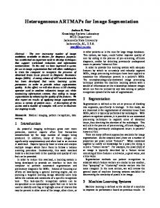
4.1.2. Occlusions Occlusions cover all cases where another tree is in the background, and the texture edge is not immediately obvious. Figure 13 shows five simulated occlusions, where the target tree on the left side of each image is a fixed distance R from the camera, and the occluded tree is a relative distance k*R from the camera (where k is a real number greater than 1). The simulated occlusions were created by taking a window of tree data, then reducing this window size by first convolving the window with an appropriate low pass filter to remove possible aliasing effects, then sampling the window both vertically and horizontally. Figure 13 shows that the correct edge can be found up until the occluded tree is a distance of 1.4*R from the camera. At this point, even humans have some trouble finding the texture edge because the occluded tree simply looks too much like the target for good segmentation. So, the algorithm incorrectly finds the outside edge in this case. However, it must be noted that this simulation was made as difficult as possible by making the mean intensity of the occlusion the same as the target, which in a real setting, will not typically happen. Also, in practice, due to limited depth of field of the camera, the occluded tree will be blurred, making the segmentation easier. A second, more difficult scenario occurs when the target almost fully occludes the background tree, and there is only a small amount of occlusion information present. If in a typical image, the target takes up approximately 30% of the horizontal resolution, and a typical occlusion like those in Figure 13 take up 6-8%, an occlusion with limited information takes up only 2% or less of the horizontal resolution. Figure 14 shows examples of this case. The first image shows the correct segmentation of an occluded region containing the same mean and standard deviation as the target taking up only 0.8% of the total horizontal resolution. The second and third images show correct 23

Distance to occlusion: 3.3*R Error:-1 Pixel

Distance to occlusion: 2*R Error: +3 Pixels

Distance to occlusion: 2.5*R Error: -3 Pixels

Distance to occlusion: 1.7*R Error: -1 Pixel

Distance to occlusion: 1.4*R Error: >5 Pixels

Figure 13: Occlusions

segmentation for tree occlusions at different distances. However, the last image shows that when the occlusion is closer than 2*R, and there is less than 1.5% of the occlusion information present, there is simply not enough information for correct segmentation, and the white background is chosen. The reason for this is that as an occlusion gets closer to the target, texture elements in the image get bigger due to the occlusion being closer to the camera. If the region containing the occlusion information is not big enough to capture these texture elements, then there is simply not enough information for correct segmentation. Therefore, the closer an occlusion is the more information is needed.

Region with same mean and standard deviation as target Coverage: 0.8% Error: 0 Pixels

Distance to Occlusion: 3.3*R Coverage: 0.8% Error: +1 Pixel

Distance to Occlusion: 2*R Coverage: 1.6% Error: +2 Pixels

Distance to Occlusion: 2*R Coverage: 0.8% Error: > 5 Pixels

Figure 14: Occlusions with limited texture information

4.1.3. Shadows The final class of texture edges is due to shadows. Forest scenes will always have shadows 24

because of leaves and branches in the canopy blocking the ambient light. If the shadows are random yet fairly uniform along the trunk, like those caused by leaves, the shadows simply look like another type of texture. Problems arise when shadows are structured and mimic a vertical edge, like those cast by thick branches. Figure 15 shows three possible shadow situations.

Shadow: Within training set Error: 0 Pixels

Shadow: Only at tree edge Error: > 5 Pixels

Shadow: Gradient at tree edge Error: > 5 Pixels

Figure 15: Shadows

The first image in Figure 15 shows a shadow being cast near the center. Since the shadow occurs within the training set, the algorithm can correctly compensate for it. But, if the shadow is right near the edge, as in the second image, this intensity shift will fool the algorithm into seeing this as a close occlusion situation. Finally, the third case shows a situation where a shadow is causing an intensity gradient near the edge. The algorithm is optimized to look for abrupt, vertical edges, so a gradient fools it into latching onto the first strong edge it can find which is a branch in the background. Using abrupt changes in intensity to signal texture boundaries is both a strength and a drawback of this algorithm. Since some of the statistics used in measuring texture are not invariant to linear gray level transformations (i.e. energy, mean), the algorithm can trigger on abrupt intensity changes, which in many cases can aid in segmentation. However, the cases in Figure 15 show that shadows on the trunk can be harmful as well, since intensity changes do not always mean texture changes.

4.2. Field Results Next, the system was taken out into a forest to collect actual data. The following are the results of a survey run consisting of 10 trees taken in a single afternoon. Care was taken to not help out the algorithm by placing the camera so that there were no occlusions. Instead, the camera was placed randomly, mimicking the images that would be taken by a surveyor. In order to give a ground truth to the results of the system, an accuracy verification step, shown in 25

Figure 16 with dotted lines, was added. Here, a tape measure was used to measure the circumference of the trunk at breast height, which was then converted to a diameter by assuming a circular cross section.

Range Measurements

Images 1-10

True Circumference Measurements

Segmentation Results

Diameter Estimate

Diameter Estimation Error

Figure 16: Field Test - Estimation Accuracy Verification

Image Number

Range

Width in Pixels

True Diameter

Est. Diameter

Estimation Error

1

3.05m

190

0.62m

0.6297m

+0.97cm

2

3.10m

151

0.48m

0.4975m

+1.75cm

3

3.4m

101

0.35m

0.3552m

+0.52cm

4

5.25m

125

0.68m

0.6876m

+0.76cm

5

6.30m

100

0.66m

0.6513m

-0.87cm

6

3.00m

119

0.37m

0.3728m

+0.28cm

7

4.25m

111

0.50m

0.4906m

-0.94cm

8

3.65m

140

0.54m

0.5398m

-0.02cm

9

4.95m

139

0.71m

0.7265m

+1.65cm

10

4.70m

108

0.55m

0.5270m

-2.30cm

Table 2: Field Test Results As is shown in Table 2, the diameter estimation error is within the required specification of one inch for all trials. One caveat to these results is that the afternoon this system was test run happened to be overcast, which did not produce shadows like those in section 4.1.3. Therefore,

26

while not a rigorous test, the field results show that this system is accurate under randomly occurring natural conditions.

27

5. Conclusions A system has been designed that can reliably estimate the diameter of a target tree simply by carrying the unit into the forest and orienting it properly in front of the trunk. This solution combines a spot laser rangefinder to measure range with a monochrome camera which can measure angular size if a captured image can be segmented into target tree and background. A new segmentation algorithm was presented that can both compensate for a non-planar target tree and can successfully segment when presented with occlusions of similar looking trees in the background. This algorithm uses the concept of the Mahalanobis difference to compensate for the non-planar surface of the tree and correctly find a small window that must contain the tree edge. Then, the exact edge location in this small window is found by using information already in the co-occurrence matrix for this window. The system has been shown to work reliably in the field and with many different simulated backgrounds. But, as described, this system has trouble in three cases. First, and least problematic, section 4.1.2. shows that the algorithm has trouble finding a texture edge when presented with a very close occlusion. At this point, even humans have some trouble finding this edge, so it is not surprising that the edge finding algorithm does too. However, trees on a plantation are regularly spaced and naturally occurring trees have a rough inter-tree spacing due to competition for sunlight. So, to ensure correct segmentation, the user can be constrained to keep the system roughly within this inter-tree distance. This will cause the occluded tree to be at least as far from the target as the target is from the camera (i.e. 2*R), which according to the simulated results, is distinguishable. So, even though the algorithm fails on cases closer than 2*R, it does not have to happen in practice. Second, section 4.1.2. also shows the failure to find texture edges given a lack of sufficient occlusion information. In the case where a background tree is almost fully occluded, and only a narrow region of occlusion information is present, there is often not enough texture information for reliable segmentation. If an occlusion is at a distance 2*R, at least 1.6% horizontal resolution coverage is necessary for accurate segmentation. Therefore, it is reasonable to require the user to set up the unit even closer to the target than required for close occlusions. This means that less occlusion information is needed for correct segmentation, and if a mistake is made, the difference between the target edge and the occlusion edge is so small to be within the 1 inch error criteria. Also, these tests were done without taking limited depth of field of the camera into account. In 28

practice, the occluded trees will be blurred making the segmentation easier, and requiring less occlusion information than shown in the worst case simulation. Finally, section 4.1.3. describes the effects of certain shadows on system performance. Natural scenes do not have reliable lighting, so for true robustness, the system should be able to work in any lighting conditions. But, as shown, if there are shadows cast near the edge of the tree, the texture edge caused by the shadow will typically be chosen over the true tree edge. One possible solution is to use a strobe flash when taking the scene image, which will remove all shadowing effects as well as help illuminate the target. Another solution, presented by Ollis and Stentz, is a method of shadow removal by using information from a color camera to compensate for the difference in spectral power distribution between light illuminating the shadowed and unshadowed regions [11]. It is possible that this method could be applied here. To summarize, this system has shown to be accurate and reliable if the system is set up so that occlusions are at a distance of 2*R or greater from the target and there are no structured shadows outside the training set. The first requirement is quite acceptable since typical forests have an average inter-tree distance set by nature. If the unit is set anywhere within this inter-tree distance, then the 2*R requirement is easily met. However, this system, like other outdoor vision systems, is hampered by poor lighting. One way to deal with shadows is to use a strobe flash, or to use a color camera and implement the Ollis-Stentz shadow compensation.

29

6. References [1]

J. Brodie, C. Hansen, and J. Reid, "Size Assesment of Stacked Logs via the Hough Transform", Transactions of the ASAE. Vol. 37(1):303-310

[2]

Criterion and Impulse Survey Lasers, Laser Technology Inc., 7070 South Tucson Way, Englewood, CO 80112

[3]

R. Duda and P. Hart, Pattern Classification and Scene Analysis, Stanford Research Institute, Menlo Park, CA, Jon Wiley and Sons, New York, 1973, pp 27-30

[4]

R.M. Haralick, K. Shanmugam, and I. Dinstein, "Texture Features for Image Classification". IEEE Transactions on Systems, Man, and Cybernetics, Vol. SMC-3, No. 6, 1973, pp. 610-621

[5]

B.K.P. Horn, Robot Vision, Cambridge MA, MIT Press, New York, McGraw Hill 1986, pg 140.

[6]

M. Kass, A. Witkin, D. Terzopoulos, "Snakes: Active Contour Models", International Journal of Computer Vision, 1988, pp 321-331

[7]

C. Kervrann and F. Heitz, "A Markov random field model based approach to unsupervised texture segmentation using local and global spatial statistics", Technical Report 752, IRISA, Campus Universitaire de Beaulieu, August 1993

[8]

H. Kreyszig, "Descriptors for Textures", Technical Report, University of Toronto, Department of Computer Science, RBCV-TR-90-33, July 1990

[9]

J. Krumm and S. Shafer, "Segmenting textured 3D surfaces using the space/frequency representation", Spatial Vision, Vol. 8, No. 2 pp. 281-308 (1994)

[10]

S. Livens, P. Scheunders, G. Van de Wouwer and D. Van Dyck, "Wavelets for Texture Analysis: An Overview", Technical Report, VisieLab, Department of Physics, RUCA University of Antwerp, April 1997

[11]

M. Ollis, A. Stentz, "Vision-Based Perception for an Automated Harvester", Proceedings of IEEE/RSJ International Conference on Intelligent Robotic Systems (IROS ’97)

[12]

Y. Rubner, C. Tomasi, "Coalescing Texture Descriptors", Proceedings of ARPA Image Understanding Workshop, February 1996

[13]

H. Voorhees and T. Poggio, "Computing texture boundaries from images", Nature 333, 364-367

[14]

S.C Zhu, T.S. Lee, A.L. Yuille, "Region Competition: Unifying Snakes, Region Growing, Energy/Bayes/MDL for Multi-band Image Segmentation", Proceedings of the Fifth International Conference in Computer Vision (ICCV ’95), pp 416-425

30