Overlapping image segmentation for context

Overlapping image segmentation for context-dependent anomaly detection James Theiler and Lakshman Prasad Space and Remote Sensing Sciences Group, Los Alamos National Laboratory, Los Alamos, NM, USA ABSTRACT The challenge of finding small targets in big images lies in the characterization of the background clutter. The more homogeneous the background, the more distinguishable a typical target will be from its background. One way to homogenize the background is to segment the image into distinct regions, each of which is individually homogeneous, and then to treat each region separately. In this paper we will report on experiments in which the target is unspecified (it is an anomaly), and various segmentation strategies are employed, including an adaptive hierarchical tree-based scheme. We find that segmentations that employ overlap achieve better performance in the low false alarm rate regime. Keywords: image segmentation, anomaly detection

1. INTRODUCTION When it comes to detecting anomalies, context is everything. Anomalies, by and large, are unspecified entities, defined only by what they are not. An anomaly is something that stands out from its background, that differs from the context in which it finds itself. When it comes to detecting anomalies in hyperspectral imagery, a wide variety of algorithms have been proposed, many of which are described in recent surveys.1, 2 These algorithms identify a context (sometimes local, sometimes global, sometimes a combination thereof), and seek to characterize the pixels in that context. Pixels that are inconsistent with their associated characterizations are identified as anomalies. The RX algorithm3 provides both a standard benchmark and an illustrative example. In the simplest variant, the context is the whole image, and the characterization is a Gaussian distribution, fit to the sample mean and sample covariance of the pixels in the image. The anomalousness of a pixel is defined by the Mahalanobis distance from the pixel to the centroid of the distribution. A slightly more complicated (and considerably more common) variant uses a moving window as its context. In particular, the anomalousness of a given pixel is based on the mean and covariance of the pixels in an annulus that surrounds that pixel. A smaller context is generally more uniform, which means that smaller deviations from what is normal can be detected. A local context is also appropriate for identifying local anomalies. A green tree in a forest is not unusual; a green tree in the desert may be. If a large image has both forest and desert areas, the lone tree in the desert may still be interesting, but only because it is unusual with respect to its local context. Detecting anomalous changes follows the same idea.4–23 In this case there are two (or more) co-registered images, and one seeks the pixel locations for which the corresponding pixels are anomalously changed; i.e., they differ in a way that different from the way all the other corresponding pixels in the images differ. For residualbased anomalous change detectors – of which chronochrome4 is the most well known, but multivariate alteration detection5 and covariance equalization7 are well known alternatives – a single image is obtained (in some cases,6 that image is explicitly the difference between the two images), and anomalies are sought in that single difference or residual image. In machine-learning approaches to anomaly detection,24–29 formal approaches have been identified that implicitly model the underlying distribution, without assuming that it has a particular parametric (e.g., Gaussian) E-mails: [email protected], [email protected]

form. (What one explicitly models is not the distribution, per se, but a boundary that encloses a large fraction of the measure in the distribution.) A strength of these approaches is that they recognize and deal with the non-Gaussian structure of real hyperspectral data. A weakness, however, is that they treat the hyperspectral image as a “bag of pixels,” without respect to the considerable spatial structure that is evident in imagery. For anomaly detection in multispectral and hyperspectral imagery, a variety of approaches have been pursued,30–40 some involving more sophisticated modeling of the spectral, and others combining spatial aspects of the imagery. In what follows, we will emphasize spatial analysis, and in particular will consider approaches employing image segmentation to limit the context under which anomalousness is sought. The spectral analysis will be standard RX, with sample mean and sample covariance provided by the data in each of the image segments. Also, although interesting anomalies might span a number of adjacent pixels, and although that is something that might be exploited in a more comprehensive anomaly detector, we will consider single pixel and sub-pixel anomalies. That is not to say that the algorithms will be useless against multi-pixel anomalies, just that they will be designed for and evaluated against anomalies with no spatial extent. In other words, it is the spatial properties of the background that we seek to exploit, not the spatial properties of the anomalous targets.

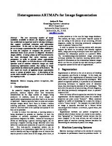
2. SEGMENTATION-BASED ANOMALY DETECTION 2.1. Fixed window segmentation In the most straightforward use of segmentation, the image is partitioned into disjoint sets of pixels (which we will call segments), and anomalies are sought separately in each segment. In particular, a mean and covariance is computed separately for each segment, and an Mahalanobis distance-based anomalousness is computed for each of the pixels in that segment. For example, one can very simply and cheaply segment an image into non-overlapping rectangular (typically square) tiles. Given that segmentation, Algorithm 1 describes the process of computing mean and covariance over each segment (i.e., in this example, over each tile), and then computing anomalousness for each pixel in that segment with respect to the mean and covariance associated with that segment. We will use square tiles as a kind of baseline to compare more sophisticated segmentations against. Algorithm 1 Anomaly detection over a segmented image. A segmentation is usually maintained as an image s for which s(j, k) is an integer index indicating the segment to which (j, k) belongs. Require: Image a, Segmentation s for each segment i do Let X ← {(j, k) | s(j, k) = i} {Set of pixels in ith segment} {Compute mean and covariance of the pixels in the segment X} P µ ← (j,k)∈X a(j, k)/|X| P R ← (j,k)∈X (a(j, k) − µ)(a(j, k) − µ)T /|X| {Compute anomalousness of each pixel in the segment X} for each pixel (j, k) ∈ X do A(j, k) = (a(j, k) − µ)T R−1 (a(j, k) − µ) end for end for Output is anomalousness image A When the segments are small, there is often concern that the anomaly being tested will contaminate the estimates of mean and covariance (as they do in other kinds of target detection41, 42 ). But when the contamination is the target itself, the effect is more benign.43 Fig. 1 shows that the effect of contamination can be quite large, but that the effect is only one of calibration. There is a monotonic relationship between the anomalousness measures computed with and without the pixel, and that relationship is constant over the whole image, so relative anomalousness over the pixels in the image is the same in either case.

Uncontaminated anomalousness

70 60

p=1 p=2 p=3 p=4

50 40 30 20 10 0 0

5 10 Contaminated anomalousness

15

Figure 1. Plot of anomalousness as computed with (horizontal axis) and without (vertical axis) the contaminating effect of the anomaly under test. The top curve is for N = 10 pixels (plus one contaminating pixel), the middle curve is for N = 20, and the bottom is for N = 50. The points correspond to trials in which N + 1 points are chosen at random, with the last point treated as the pixel under trial. Trials are performed for dimensions p = 1 through p = 4. The lines are ˜ ˜ ) where A is the uncontaminated anomalousness, and A˜ is the contaminated value. the curves A = A/(1 − A/N

2.1.1. Adaptive and hierarchical segmentation While tile-based segmentations are simple and cheap to obtain, they do not exploit the detailed spatial structure in the image. (They do exploit the general tendency for parts of the image that are far apart spatially to be less correlated spectrally.) Purely spectral segmentation, such as k-means,44–46 provide clusters of pixels that are not necessarily adjacent, but that can in principle still be used for anomaly detection. However, this is not very effective for finding single pixels that are locally anomalous, because locality is not taken into account. Variants of k-means that account for spatial structure, such as contig-k-means,47 or the superpixels given by simple linear iterative clustering (SLIC),48 are more promising for this purpose, but will not be pursued here. Our focus here will be on a particular segmentation algorithm, known as HierArchitect,49–51 which produces not a single segmentation but a stack of them. This segmentation scheme starts with image edges as a prior and establishes proximity-based regional relationships between them via a Delaunay triangulation. The triangles are then grouped into polygons based on region-contour affinity criteria. The grouping criteria tend to assemble spectrally similar areas with relatively smooth boundaries. They are grouped further based on their individual and ensemble spatio-spectral characteristics, thus generating nested polygons at multiple scales. By choosing a particular level of the hierarchy, a finer or coarser segmentation can be obtained. And this segmentation, just like that of the fixed tile segmentation, can be taken as input to Algorithm 1 for finding anomalies in the image.

2.2. Detectors based on overlapping segmentations One difficulty with fixed segmentations is that pixels near the borders of segments may be “less typical” than pixels well into the interior, and may appear as false positives in segmentation-based anomaly detection. Furthermore, particularly with the adaptive segmentation schemes, there may be boundary effects of quantization due to rasterization. We suggest that these problems can be dealt with using algorithms based on overlapping segmentations. For example, a pair of overlapping square tile segmentations leads to the “double-window detector” described in Algorithm 2. The basic idea is to compute two anomalousness maps, one for each segmentation, and then to take the pixel-by-pixel minimum to produce the final anomalousness map.

Algorithm 2 Double-window anomaly detection Require: Image a, Two segmentations s1 , s2 Compute A1 using segmentation s1 in Algorithm 1 Compute A2 using segmentation s2 in Algorithm 1 for each pixel (j, k) in the image do A(j, k) ← min(A1 (j, k), A2 (j, k)) end for An approach which combines the utility of overlapping segmentations with the image-adaptability of the hierarchical segmentation is described in Algorithm 3. Here, each of the segments is made just a little bit larger (in our experiments, we dilated by just two pixels), so as to more completely cover the boundary region. As with the double-window detector, the anomalousness of pixels that are covered by multiple segments is computed by taking the minimum of all the anomalousness values computed for that pixel. Algorithm 3 Anomaly detection with dilated segments Require: Image a, Segmentation s, Dilation d {Here, d is the structuring element for the dilation.} Initialize anomalousness image A ← ∞ for each segment i do Let X ← {(j, k) | s(j, k) = i} {Set of pixels in ith segment} Let b be a binary image, with b(j, k) = 1 for (j, k) ∈ X and zero otherwise. b ← dilate(b, d) {Dilate the binary mask} Let X 0 ← {(j, k) | b(j, k) = 1} {Expand X to include pixels within a distance d of X} {Compute mean and covariance of the pixels in the segment X 0 } {Compute anomalousness A0 of each pixel in the segment X 0 } for each pixel (j, k) ∈ X 0 do A(j, k) = min(A(j, k), A0 (j, k)) end for end for Output is anomalousness image A

2.3. Moving window detector The moving window anomaly detector can be thought of as an extreme case of an overlapping segmentation. A separate mean and covariance are computed for every pixel in the image, based on the pixels in a window that is centered on that pixel. A naive implementation of the moving window anomaly detector can be very expensive. If there are N pixels in a p-channel image, and a window of width w is employed, then there will be O(N p2 w2 ) + O(N p3 ) operations to compute the covariance matrices at all the pixels. The implementation in Algorithm 4 speeds this up considerably. The local outer products require O(N p2 ) operations; depending on the implementation of the smoothing operator, up to O(N pw2 ) operations are necessary, and much fewer if Fourierbased smoothing (which is standard in packages like Matlab) is used. Finally, the anomalousness computations only take O(N p3 ) operations (since all of those covariances matrices need to be inverted). In practice, it is the O(N p3 ) terms that dominate, but that is the same order as an estimate of anomalousness based on a single global estimate of the covariance.

3. SIMULATED IMAGERY For real imagery, there is no “ground truth” with respect to the correct hierarchical segmentation. So we will begin with simulated imagery where that decomposition is built into the simulation. The simulated image has a fractal structure based on nested quad-trees, optionally followed by a rotation. In the first step, the image is divided into quadrants, each quadrant is assigned a random value, and that value is assigned to all the pixels in the quadrant. Each quadrant is divided into sub-quadrants, and each of those sub-quadrants is assigned a random value, and that value is added to all the pixels in the sub-quadrant. The process continues until the

Algorithm 4 Anomaly detection with moving window Require: p-channel image a, window width w Create temporary image z with p(p + 1)/2 channels. a ← a − mean(a) {Subtract mean from image; this is not strictly necessary, but is numerically advantageous.} for each pixel (j, k) in the image do Compute R ← a(j, k)a(j, k)T ∈ Rp×p Pack the p(p + 1)/2 distinct components of R into z(j, k) end for z ← smooth(z, w) {Smooth image z in place, using a w × w square window} a ← a − smooth(a, w) {Subtract local mean from image a} for each pixel (j, k) in the image do Unpack components of z(j, k) into symmetric matrix R ∈ Rp×p R ← R − a(j, k)a(j, k)T A(j, k) ← a(j, k)T R−1 a(j, k) {Mahalanobis distance to local mean is anomalousness} end for Output is anomalousness image A

(a) Square (θ = 0)

(b) Rotated (θ = 30o )

Figure 2. The first band of two simulated images, with and without rotation, illustrating the hierarchical structure that is designed into Algorithm 5. One can see structure on all scales, as well as strong (and weak) edges. Both images are 1024×1024 pixels and were generated using γ = 0.5.

sub-sub-· · ·-sub-quadrants are individual pixels. An implementation is described in Algorithm 5, and an example is shown in Fig. 2(a). A variant is to start with an image twice as large as desired, to rotate it by some angle θ, and then to crop the center of the rotated image, as seen in Fig. 2(b). Algorithm 5 Simulating one band of a fractal square image of size 2n on a side. Multi-band images can be made using the same scheme (with different random number seed) for subsequent bands. The larger γ, the more distinct are the larger squares; we used γ = 0.5. Require: Parameters n, γ, θ a(1 : 2n+1 , 1 : 2n+1 ) ← 0; {Initialize double-sized image with zeros} for i = 1 to n + 1 do w ← 2n+1−i {width of square; there will be 4i of these squares, corresponding to the ith level of a quad-tree.} for j = 1 to 2i do Rj ← [1 + (j − 1)w : jw]; {range of row indices} for k = 1 to 2i do Rk ← [1 + (k − 1)w : kw]; {range of column indices} {Note: (Rj , Rk ) is a range that covers a square of width w} Let r be a random scalar {We use a Gaussian distribution} a(Rj , Rk ) ← a(Rj , Rk ) + wγ r {Add random value to square of width w} end for end for end for a ← rotate(a, θ) {Rotate image by angle θ} Let (c, c) be the center of the rotated image Rc = [1 + c − 2n−1 : c + 2n−1 ] {Range of 2n indices centered at c} a ← a(Rc , Rc ) {Crop out the central 2n × 2n pixels}

3.1. Simulating anomalies Starting either from a simulated or a real image, anomalies can be artificially embedded in the image so that algorithms for detecting anomalies can be quantitatively evaluated. Our approach for this simulation is to draw from the image itself. Our anomalies are not spectrally anomalous with respect to the entire image; indeed, they are typical in this global context by definition, since they are drawn at random from the image. However, by placing the pixels in new random locations – the details are shown in Algorithm 6 – we will generate local anomalies, pixels that are not by themselves unusual, but are unusual with respect to their local context. In the experiments reported here, m = 1049 anomalies were generated; this corresponds to 1/1000 of the total number of pixels. Algorithm 6 Simulating full (α = 1) and sub-pixel (α < 1) anomalies; this algorithm inserts m anomalous pixels into the image a. These anomalies are obtained from random positions in the same image. Require: Image a, Parameters m, α Choose m random pixels locations in the image a: (j1 , k1 ), . . . , (jm , km ) Let b(1), . . . , b(m) be the pixel values a(j1 , k1 ), . . . , a(jm , km ). Let p(1), . . . , p(m) be a random permutation of the integers {1, . . . , m}. for i = 1 to m do Set a(ji , ki ) ← (1 − α)a(ji , ki ) + αb(p(i)) end for

4. RESULTS With simulated images and simulated anomalies, we are able to evaluate and compare the different segmentationbased anomaly detectors that we have discussed.

(a)

(b)

(c)

(d)

Figure 3. (a,b) Segmentation using HierArchitect on the simulated square and rotated images shown in Fig. 2. (c) Fixedwindow segmentation does not pay attention to the content of the image, so it is the same for both images. (c,d) The double-window segmentation combines the anomalousness maps of two fixed-window segmentations, each offset from the other by half the width of the square. The colors in these segmentations are randomly chosen and serve only for visualization purposes.

(a) square

(b) rotated

1

1

0.8 Detection Rate

Detection Rate

0.8

0.6

0.4 MovingWindow FixedWindow DoubleWindow HierArchitect HierArchitect(dilated)

0.2

0 −6 10

−5

10

−4

−3

−2

10 10 10 False Alarm Rate

−1

10

MovingWindow FixedWindow DoubleWindow HierArchitect HierArchitect(dilated)

0.6

0.4

0.2

0

10

0 −6 10

−5

10

−4

−3

−2

10 10 10 False Alarm Rate

−1

10

0

10

Figure 4. ROC curves for local anomaly detection in simulated images, using a variety of strategies. The original images are 1024×1024 pixels, and are based on the simulation illustrated in Fig. 2(a) and Fig. 2(b). The anomalies are single-pixels that were simulated by sampling randomly from across the image.

For the unrotated image in Fig. 2(a), there is a fortuitous (and unnatural) alignment of the natural hierarchy of the image with the image axes. This means, for instance, that tile-based segmentation (especially if those tiles are squares whose widths are powers of two) will very neatly match the built-in segments in the simulated image. One consequence of this alignment is seen in within-segment variances shown in Table 1. In general, the smaller the within-segment variances, the better, because less clutter means anomalies are more detectable. We see that with the fixed window segmentation leads to low variance for the unrotated image. The moving window is also aligned with the natural hierarchy, but it does not have as low a variance because although the axes are aligned, the offsets generally are not. The HierArchitect segmentation (which is seen in Fig. 3(a)) is smaller still, partly because the boundaries have been adapted to the image content (but possibly also because, at this level of the hierarchy, there were more segments than for the fixed window). The dilated segmentation has substantially higher variance, nominally suggesting that its performance should be worse than the original HierArchitect segmentation. Fig. 4(a) shows the actual performance, as defined in terms of detections and false alarms. It shows excellent performance for the fixed window detector, and only marginally better performance for the much lower-variance segmentation given by HierArchitect, and that marginal improvement only coming in the high false-alarm rate regime. At lower false alarm rates, the HierArchitect solution is the worst of all the plotted alternatives. That this can be attributed to effects on the border of the segments is indicated by the substantially better performance at low false alarm rate exhibited by the dilated HierArchitect. The rotated case should be considered more typical, because the fortuitous alignments no longer apply. In this example, looking again at Table 1, the square window variances are much larger than the adaptive HierArchitect variances, even though those windows are on average smaller. And in this case, Fig. 4 shows that in the moderate false alarm rate regime (larger than 10−3 ), the HierArchitect performance is substantially better than any of the square window variants. Also, in this unaligned case, we see that the moving window and double-window detectors outperform the fixed window detector, and this is seen over the full range of false alarm rates. As with the aligned case, we also see that the small two-pixel dilation dramatically improves the low false alarm rate performance of the HierArchitect detector.

5. CONCLUSIONS To investigate and compare the effectiveness of segmentation-based anomaly detectors, we developed a way to simulate imagery that builds in a natural hierarchical structure. We also proposed a principled scheme to simulate anomalies in a way that tests for local anomalousness without confounding that with global anomalousness. Based

Segmentation Algorithm Moving window Fixed window HierArchitect HierArchitect (dilated)

Number of Segments Square Rotated – – 64 64 99 41 99 41

Within-segment variance Square Rotated 367 543 111 461 83 130 144 181

Table 1. Number of segments and average within-segment variances for four segmentations. Although the moving window has a huge number of (highly overlapping) segments, it is the same size as the fixed window, which has a width of 128 pixels.

on this imagery and these anomalies, we produced ROC curves that quantified the performance of different detection algorithms in terms of detection and false alarm rates. One conclusion to be drawn from the performance of the detectors in Fig. 4 is that overlapping segmentations outperform disjoint segmentations in the low false alarm rate. The tendency of false alarms to concentrate on the boundaries of segments is a problem that has been previously noted,52–54 and the effect of the overlapping segments is to ameliorate these boundary effects. The ostensible problem with the moving window (aside from the computational expense) is that a window that straddles two natural segments of an image will have larger variance than is needed to express the natural variability expected at the center pixel, thereby reducing the magnitude of anomalousness that is detectable. This effect is exhibited as reduced performance for the moderate false alarm rate regime, compared to adaptive segmentation, such as that given by the HierArchitect. But the moving window has a robustness against false alarms because the pixel under test is always far from the boundary, and this is seen in the respectable performance at low false alarm rate. In this paper, we introduced two tricks for improving the performance of segmentation-based anomaly detection: the double-window (or twindow !) trick, and the dilation trick. Both tricks involve overlapping segments, and this overlap minimizes the false alarms that occur on the boundaries of segments. These methods are competitive with the moving window algorithm, but are much cheaper. And in the case of the dilated HierArchitect, we can combine the advantages of adaptive segmentation with the robustness of these overlaps to produce a detector the performs well across the whole range of false alarm rate.

Acknowledgments This work was supported by the Laboratory Directed Research and Development (LDRD) program at Los Alamos National Laboratory. We are grateful to Jacopo Grazzini for useful discussions, and for pointing out Ref. [48].

REFERENCES 1. D. W. J. Stein, S. G. Beaven, L. E. Hoff, E. M. Winter, A. P. Schaum, and A. D. Stocker, “Anomaly detection from hyperspectral imagery,” IEEE Signal Processing Magazine 19, pp. 58–69, Jan 2002. 2. S. Matteoli, M. Diani, and G. Corsini, “A tutorial overview of anomaly detection in hyperspectral images,” IEEE A&E Systems Magazine 25, pp. 5–27, 2010. 3. I. S. Reed and X. Yu, “Adaptive multiple-band CFAR detection of an optical pattern with unknown spectral distribution,” IEEE Trans. Acoustics, Speech, and Signal Processing 38, pp. 1760–1770, 1990. 4. A. Schaum and A. Stocker, “Long-interval chronochrome target detection,” Proc. ISSSR (International Symposium on Spectral Sensing Research) , 1998. 5. A. A. Nielsen, K. Conradsen, and J. J. Simpson, “Multivariate alteration detection (MAD) and MAF postprocessing in multispectral bi-temporal image data: new approaches to change detection studies,” Remote Sensing of the Environment 64, pp. 1–19, 1998.

6. L. Bruzzone and D. F. Prieto, “Automatic analysis of the difference image for unsupervised change detection,” IEEE Trans. Geoscience and Remote Sensing 38, pp. 1171–1182, 2000. 7. A. Schaum and A. Stocker, “Linear chromodynamics models for hyperspectral target detection,” Proc. IEEE Aerospace Conference , pp. 1879–1885, 2003. 8. C. Clifton, “Change detection in overhead imagery using neural networks,” Applied Intelligence 18, pp. 215– 234, 2003. 9. A. Schaum and E. Allman, “Advanced algorithms for autonomous hyperspectral change detection,” IEEE Applied Imagery Pattern Recognition (AIPR) Workshop: Emerging technologies and applications for imagery pattern recognition 33, pp. 33–38, 2005. 10. J. Theiler and S. Perkins, “Proposed framework for anomalous change detection,” ICML Workshop on Machine Learning Algorithms for Surveillance and Event Detection , pp. 7–14, 2006. 11. J. Theiler and S. Perkins, “Resampling approach for anomalous change detection,” Proc. SPIE 6565, p. 65651U, 2007. 12. A. A. Nielsen, “The regularized iteratively reweighted MAD method for change detection in multi- and hyperspectral data,” IEEE Trans. Image Processing 16, pp. 463–478, 2007. 13. M. T. Eismann, J. Meola, and R. Hardie, “Hyperspectral change detection in the presence of diurnal and seasonal variations,” IEEE Trans. Geoscience and Remote Sensing 46, pp. 237–249, 2008. 14. J. Meola and M. T. Eismann, “Image misregistration effects on hyperspectral change detection,” Proc. SPIE 6966, p. 69660Y, 2008. 15. J. Theiler, “Sensitivity of anomalous change detection to small misregistration errors,” Proc. SPIE 6966, p. 69660X, 2008. 16. J. Theiler, “Subpixel anomalous change detection in remote sensing imagery,” Proc. IEEE Southwest Symposium on Image Analysis and Interpretation , pp. 165–168, 2008. 17. M. T. Eismann, J. Meola, A. D. Stocker, S. G. Beaven, and A. P. Schaum, “Airborne hyperspectral detection of small changes,” Applied Optics 47, pp. F27–F45, 2008. 18. J. Theiler, “Quantitative comparison of quadratic covariance-based anomalous change detectors,” Applied Optics 47, pp. F12–F26, 2008. 19. L. Prasad and J. Theiler, “A structural framework for anomalous change detection and characterization,” Proc. SPIE 7341, p. 73410N, 2009. 20. J. Theiler, N. R. Harvey, R. Porter, and B. Wohlberg, “Simulation framework for spatio-spectral anomalous change detection,” Proc. SPIE 7334, p. 73340P, 2009. 21. J. Theiler, C. Scovel, B. Wohlberg, and B. R. Foy, “Elliptically-contoured distributions for anomalous change detection in hyperspectral imagery,” IEEE Geoscience and Remote Sensing Letters 7, pp. 271–275, 2010. 22. I. Steinwart, J. Theiler, and D. Llamocca, “Using support vector machines for anomalous change detection,” Proc. IEEE International Geoscience and Remote Sensing Symposium (IGARSS) , pp. 3732–3735, 2010. 23. M. T. Eismann, J. Meola, and A. D. Stocker, “Automated hyperspectral target detection and change detection from an airborne platform: Progress and challenges,” Proc. IEEE International Geoscience and Remote Sensing Symposium (IGARSS) , pp. 4354–4357, 2010. 24. S. Ben-David and M. Lindenbaum, “Learning distributions by their density levels: A paradigm for learning without a teacher,” J. Computer and System Sciences 55, pp. 171–182, 1997. 25. D. Tax and R. Duin, “Data domain description by support vectors,” in Proc. ESANN99, M. Verleysen, ed., pp. 251–256, D. Facto Press, (Brussels), 1999. 26. B. Sch¨ olkopf, J. Platt, J. Shawe-Taylor, A. J. Smola, and R. C. Williamson, “Estimating the support of a high-dimensional distribution,” Neural Computation 13, pp. 1443–1471, 2001. 27. T. Hastie, R. Tibshirani, and J. Friedman, Elements of Statistical Learning: Data Mining, Inference, and Prediction, Springer-Verlag, New York, 2001. This anomaly detection approach is developed in Chapter 14.2.4, and neatly illustrated in Fig 14.3. 28. D. Tax and R. Duin, “Uniform object generation for optimizing one-class classifiers,” J. Machine Learning Res. 2, pp. 155–173, 2002. 29. I. Steinwart, D. Hush, and C. Scovel, “A classification framework for anomaly detection,” J. Machine Learning Research 6, pp. 211–232, 2005.

30. H. Ren, J. O. Jensen, and Q. Du, “Efficient anomaly detection and discrimination for hyperspectral imagery,” Proc. SPIE 4725, pp. 234–241, 2002. 31. P. E. Clare, W. J. Oxford, S. Murphy, P. Godfree, V. Wilkinson, and M. Bernhardt, “A new approach to anomaly detection in hyperspectral images,” Proc. SPIE 5093, pp. 17–28, 2003. 32. J. Theiler and D. M. Cai, “Resampling approach for anomaly detection in multispectral images,” Proc. SPIE 5093, pp. 230–240, 2003. 33. H. Kwon, S. Z. Der, and N. M. Nasrabadi, “Adaptive anomaly detection using subspace separation for hyperspectral imagery,” Opt. Eng. 42, pp. 3342–3351, 2003. 34. H. Kwon and N. M. Nasrabadi, “Kernel RX: a new nonlinear anomaly detector,” Proc. SPIE 5806, pp. 35– 46, 2005. 35. M. Bernhardt, J. P. Heather, and M. I. Smith, “New models for hyperspectral anomaly detection and un-mixing,” Proc. SPIE 5806, pp. 720–730, 2005. 36. K. Ranney and M. Soumekh, “Hyperspectral anomaly detection within the signal subspace,” IEEE Geoscience and Remote Sensing Letters 3, pp. 312–316, 2006. 37. A. Banerjee, P. Burlina, and C.Diehl, “A support vector method for anomaly detection in hyperspectral imagery,” IEEE Trans. Geoscience and Remote Sensing 44, pp. 2282–2291, 2006. 38. A. Schaum, “Hyperspectral anomaly detection: Beyond RX,” Proc. SPIE 6565, p. 656502, 2007. 39. S. M. Adler-Golden, “Improved hyperspectral anomaly detection in heavy-tailed backgrounds,” Proc. IEEE Workshop on Hyperspectral Image and Signal Processing: Evolution in Remote Sensing (WHISPERS) 1, 2009. 40. J. Theiler and D. Hush, “Statistics for characterizing data on the periphery,” Proc. IEEE International Geoscience and Remote Sensing Symposium (IGARSS) , pp. 4764–4767, 2010. 41. T. E. Smetek and K. W. Bauer, “Finding hyperspectral anomalies using multivariate outlier detection,” Proc. IEEE Aerospace Conference , 2007. 42. W. F. Baesner, “Clutter and anomaly removal for enhanced target detection,” Proc. SPIE 7695, p. 769525, 2010. 43. J. Theiler and B. R. Foy, “Effect of signal contamination in matched-filter detection of the signal on a cluttered background,” IEEE Geoscience and Remote Sensing Letters 3, pp. 98–102, 2006. 44. J. MacQueen, “On convergence of k-means and partitions with minimum average variance,” Ann. Math. Statist. 36, p. 1084, 1965. (Abstract). 45. E. Forgy, “Cluster analysis of multivariate data: efficiency versus interpretability of classifications,” Biometrics 21, p. 768, 1965. (Abstract). 46. J. MacQueen, “Some methods of classification and analysis of multivariate observations,” in Proceedings of Fifth Berkeley Symposium on Mathematical Statistics and Probability, L. M. L. Cam and J. Neyman, eds., pp. 281–297, University of California Press, (Berkeley), 1967. 47. J. Theiler and G. Gisler, “A contiguity-enhanced k-means clustering algorithm for unsupervised multispectral image segmentation,” Proc. SPIE 3159, pp. 108–118, 1997. 48. R. Achanta, A. Shaji, K. Smith, A. Lucchi, P. Fua, and S. Susstrunk, “SLIC superpixels,” Tech. Rep. 149300, EPFL, June 2010. 49. L. Prasad and A. Skourikhine, “Vectorized image segmentation via trixel agglomeration,” Pattern Recognition 39, pp. 501–514, 2006. 50. L. Prasad and S. Swaminarayan, “Hierarchical image segmentation by polygon grouping,” IEEE CVPR Workshop on Perceptual Organization in Computer Vision (Anchorage, AK) , 2008. 51. L. Prasad and S. Swaminarayan, “A framework for perceptual image analysis,” IEEE Asilomar Conference on Signals, Systems and Computers (Pacific Grove, CA) 43, 2009. 52. A. Schaum, “A remedy for nonstationarity in background transition regions for real time hyperspectral detection,” IEEE Aerospace Conference , 2006. 53. A. Schaum, “Autonomous hyperspectral target detection with quasi-stationarity violation at background boundaries,” IEEE Applied Imagery and Pattern Recognition (AIPR) Workshop 35, 2006. 54. N. Gorelnik, H. Yehudai, and S. R. Rotman, “Anomaly detection in non-stationary backgrounds,” Proc. IEEE Workshop on Hyperspectral Image and Signal Processing: Evolution in Remote Sensing (WHISPERS) 2, 2010.