Approximate Schemas, Source-Consistency and Query Answering Michel de Rougemont∗, Adrien Vieilleribi`ere†
Abstract We use the Edit distance with Moves on words and trees and say that two regular (tree) languages are ε-close if every word (tree) of one language is ε-close to the other. A transducer model is introduced to compare tree languages (schemas) with different alphabets and attributes. Using the statistical embedding of [8], we show that Source-Consistency and Approximate Query Answering are testable on words and trees, i.e. can be approximately decided within ε by only looking at a constant fraction of the input.
1
Introduction
For a class K of finite structures, a Schema is a subset K0 ⊆ K, i.e. a subclass. We consider classes of strings, ordered and unordered trees and introduce the notion of Approximate Schemas, i.e. a notion to compare languages of strings or trees. We use the Edit distance with Moves on words and trees and say that two subclasses (languages) are ε-close if every word (tree) of one subclass is ε-close to the other. When the subclasses use the same alphabet, [10, 8] show, based on Property Testing, how to approximate the distance between words (trees) by sampling a number of subword independent of the size n, but only dependent on some ε parameter, and how to test regular properties in a similar way. We wish to generalize this approach to languages which do not use the same vocabulary, i.e. compare languages such as K1 = 0∗ 1∗ and K2 = c(ab)∗ ca∗ . In the classical sense K2 = c(ab)∗ ca∗ is close to K3 = (ab)∗ a∗ as every word of length n of K2 is at relative distance n2 to K3 , by deleting the two c’s, and conversely every word of K3 is at relative distance n2 to K3 , by inserting two c’s. We say K2 and K3 are ε-close for any ε, as n2 ≤ ε for large enough n. There is a simple transducer (finite state machine with one state) T which translates 0 into ab, 1 in to a, such that the image of K1 = 0∗ 1∗ , by T , i.e. T (0∗ 1∗ ) = (ab)∗ a∗ . In this case, we say that K1 and K3 are ε-similar for any ε. We introduce a model of transducer which transforms labelled trees with attributes and is well suited for XML, Data-Exchange and Data-Integration. It allows to compare schemas, XML files with different schemas and to also learn schemas from positive and negative examples. We first present the approach for words, and regular expressions as schemas, but it generalizes naturally to trees and other classes of structures. Given a word w in some alphabet Σ, a regular expression r on a different alphabet Σ0 and a deterministic transducer T , we say that w is ε-close to r via T if there exists w0 ε-close to w such that T (w0 ) is ε-close to r. In Data Exchange [7, 3], a setting is a triple (KS , T , KT ) where KS , KT are the Source and Target Schemas, and T is a binary relations between Source structures I and target structures J. Given a Data-Exchange setting, Source-Consistency takes an input Source I of size n and decides if there exists a J such that (I, J) ∈ T and J ∈ KT , whereas Query Answering takes ∗ †
[email protected], University Paris-II, CNRS-LRI,France
[email protected], LRI, University Paris-Sud, France
1
an input Source I and decides if all J such that all (I, J) ∈ T are such that J ∈ KT . We define the approximate versions when T is the binary relation associated with a transducer T . Let (KS , T , KT ), be such a Data-Exchange setting. • Approximate Source-Consistency takes I and ε as input and decides if I is ε-close to KT via T , i.e. if there exists I 0 ε-close to I and J 0 such that such that (I 0 , J 0 ) ∈ T and J 0 is ε-close to KT . • Approximate Query answering takes I and ε as input and decides if there exists I 0 ε-close to I such that all J 0 such that (I 0 , J 0 ) ∈ T are ε-close to KT . We first consider deterministic T and generalize to non deterministic transducers and transducers with nulltransitions. In the case of XML files, I is a tree and K is a DTD. We wish to decide if a given file is close or far from a DTD after transformation by a transducer. In many Data-Integration situations, the transducer needs to manage attributes, one of the motivations of our model. Property Testing is a framework to approximate decision problems, which is well suited on classes of finite structures with a distance. Given a parameter 0 ≤ ε ≤ 1, an ε-tester [14, 9] for a property P decides if a structure satisfies the property P or if it is ε-far from satisfying the property P . A property P is testable if there exists a randomized algorithm which is an ε tester for all ε > 0 and whose time complexity is independent of the size of the structure and only dependent on ε. When the structure is ε-close to the property, a Corrector finds in linear time a structure which satisfies the property and which is ε-close to the initial structure. The main results of the paper use the Edit Distance with Moves on words and trees, and a transducer model to transform structures from one language into structures of another language. We show: • Source-Consistency is testable on words and trees, i.e. for all ε there is an ε-tester which decides in time independent of n the size of I if the input I is Source-Consistent or is ε-far from being SourceConsistent. • Query Answering is similarly testable on words and trees. • If a word w is ε-close to a regular expression r via T , we can find w0 ε-close to w such that T (w0 ) is ε-close to r in linear time. These results are based on the testers and correctors for words (resp. trees) introduced in [10] for regular words (resp. regular trees) and depend on this specific Edit Distance with Moves. Other distances do not provide such results. We also use the embedding of words into statistical vectors introduced in [8] which yields natural testers to decide Equality, Membership of a regular language and a polynomial time algorithm to decide if two non-deterministic automata are ε-equivalent. A corrector for XML along this theory presented in [4], is also used. Learning regular properties on words and trees is also closely connected to these problems, using similar techniques. In section 2, we review the basic data exchange models, the approximation of decision problems provided by the ε-testers. We study approximate data exchange on words in section 3, and on trees in section 4.
2
Preliminaries
A k-ranked ordered tree with n nodes is a structure T = (Dn , Firstchild, Nextsibling, root) where the domain Dn = {1, ..., n} is the set of nodes with at most k successors. The relations Firstchild, Nextsibling are binary relations such that Firstchild(u, v) if v is the first child of u, Nextsibling(v, v 0 ) if v 0 is the next sibling of 2
v, and root is a distinguished element of Dn with no predecessors. There are at most k siblings and the graph with Firstchild and Nextsibling edges is a tree. A word w is a 1-ranked tree and the Nextsibling relation is empty. An unranked ordered tree is a structure T = (Dn , Firstchild, Nextsibling, root) without a fixed limitation on the number of siblings, which remains less than n − 1. An unranked unordered tree is a structure T = (Dn , Child, root) with no order on the siblings. We consider labelled trees with attribute values, i.e. nodes have a label (tag) and attributes with values in a set Str. Given a finite alphabet Σ and a finite set A of attributes, we consider a class KΣ,A of (Σ, A) labeled tree structures I which can be ordered or unordered. They have two domains: D is the set of nodes, and Str the set of attribute values. • On ordered trees, I = (D, Str, Firstchild, Nextsibling, root, L, λ)} • On unordered trees, I = (D, Str, Child, root, L, λ)} where root is the root of the tree, L : D → Σ defines the node label, and λ : D × A → Str is a partial function which defines the attributes values of a node, when they exist. On unordered trees Child is the edge relation of an unranked tree, whereas on ordered trees Firstchild defines the first child of a node and Nextsibling defines the successor along the siblings. Example 1: Strings, Relations and Trees as KΣ,A classes. (a) Let Σ = {0, 1}, A = ∅, D = {1, ..., n}, Str = ∅, K1 = {I = (D, Str, Child, r, L, λ)} where Child in the natural successor over D and L : D → {0, 1}. This class represents binary words of length n. If A0 = {A1 , A2 }, Str = {a, c}, we have binary words with two attributes, and values in Str. For example 1.0[A1 =a] .1[A1 =c,A2 =c] .0[A1 =a] .1.0[A1 =a] is a word where certain letters have attribute values. For example L(2) = 0 and λ(2, A1 ) = a. (b) Let Σ = ∅, A = {A1 , A2 , A3 }, D = {1, ..., n}, and Str an arbitrary set of string values, K2 = {I = (D, Str, Child, r, L, λ)}, such that Child is the edge relation of an unranked tree of depth 1 whose leaves have attributes A1 , A2 , A3 and values in Str. This class represents ternary relations with n − 1 tuples having values in Str. (c) Let Σ = {0, 1}, D = {1, ..., n}, A = ∅,Str = ∅, K3 = {I = (D, Str, Firstchild, Nextsibling, L, λ)}. This class represents unranked ordered trees with n nodes without attributes.
We consider regular schemas, i.e. classes defined by automata. For unranked ordered trees, the automata have been defined by [17] and DTDs are special cases. XML schemas define regular properties of ordered and unordered trees.
2.1
Distances
The Edit distance has been introduced in [18] for comparing strings and generalized in [16] for trees. The Edit distance between two words is the minimal number of insertions, deletions and substitutions of a letter required to transform one word into the other. The best known algorithm for computing the edit distance between two words is in O(n2 / ln n) [12]), for the time complexity. Several approximation algorithms have been proposed but no algorithm achieves an approximation with a constant error for this distance. Consider an extension of the distance: the Edit distance with moves, where arbitrary substrings can be moved in one step, as in [6, 15]. Let the relative Edit distance with moves between two strings w and w0 , written dist(w, w0 ), the minimal number of elementary operations (insertions, deletions, substitutions and moves) on w to obtain w0 , divided by max{|w|, |w0 |}.
3
v
v
v v
Node Insertion
Edge Insertion
Deletion
Delection
(c)
Rule 3: Deletion
(b)
(d)
(a)
Figure 1: Tree-Edit operations for binary trees in (a),(b),(c), and a Move operation in (d). The Tree Edit distance consider basic operations on ordered labelled trees: updating a label or an attribute, inserting a node or an edge, and deleting a node or an edge. An attribute value is considered as a label: it can be modified, entirely removed or added, at a unit cost, independent of the size of the attribute value. On ordered binary trees without labels, operations must preserve the binary tree and certain edge deletions are prohibited. Hardness results and polynomial algorithms for ordered and unordered trees, are presented in [2]. In figure 1, we obtain the tree (b) from the tree (a) with a node insertion and the tree (c) from the tree (b) with an edge insertion. The Tree Edit Distance with Moves generalizes the Edit distance with a new operation, the Move of an entire subtree from one node to another node (e.g. between (a) and (d) in figure 1). Definition 1. The Edit distance with moves between two ordered unranked trees T and T 0 , written dist(T, T 0 ), is the minimal number of elementary operations on T to obtain T 0 , divided by max{|T |, |T 0 |}. The distance between T and a language L, noted dist(T, L) is the minimum distance between dist(T, T 0 ) for T 0 ∈ L We say that two trees T and T 0 are ε-close if their relative distance is less than ε where the relative distance is the Edit distance with moves divided by M ax{|T |, |T 0 |.
2.2
Transductions
Two main approaches are used to specify transformations between a source instance and possible target instances. Let T be a binary relation defined by some pairs of structures (I, J) where I ∈ KS and J ∈ KT for a target schema KT . The transformation T can be defined by regular transductions or by formulas linking sources to targets. A transduction transforms a source structure I into a target structure J in the language of the target. It does not change the basic structure of I but transforms the tags from the source language to tags of the target language. There is a large literature on tree transducers and our model is close to the top-down tree transducers of [11], but also handles attributes values. Let KS be a set of (ΣS , AS ) trees and KT be a set of (ΣT , AT ) trees. A transducer associates in a top-down manner with a node v with label in ΣS and attribute values along attributes in AS = {A1 , ..., Ak }, a local new finite (ΣT , AT ) subtree and new attribute values for each node of that tree. In particular, a node v with attribute values A1 = a can generate a child node with label A1 and data-value a, and conversely. This setting is motivated by the XSLT language where this feature is standard. Let HΣT ,AT be the set of finite sequences of finite trees (hedges) with attributes in AT and values in Str ∪ V ar. The values of the attributes may be defined, i.e. in Str, or unknown. In this last case, we use a 4
new variable in V ar. Let HΣT ,AT [Q] be the set of finite sequences of finite trees where one leaf of each tree is a distinguished element labelled by a sequence of states in Q, which is possibly empty. The transducer is defined by three functions. The function δ defines the local tree transformation at each node, the function h defines the transformation of attribute values (into possibly null values) and the partial function µ defines the positions of the new attribute values in the new finite tree t introduced by δ. Definition 2. A tree transducer T between (ΣS , AS ) trees and (ΣT , AT ) trees is defined by (Q, q0 , δ, h, µ) where: • δ : ΣS × Q → HΣT ,AT [Q] • h : ΣS × Q × AS → {1} ∪ V ar, • µ : ΣS × Q × AT × DT → {1, 2, ...k}, where DT is the set of nodes of the sequence of trees (hedge) defined by δ. The function h extends to a function h0 : ΣS × Q × Str → Str ∪ V ar as follows. For label l ∈ LS , state q ∈ Q, if h(l, q, AiS ) = 1 then h0 (l, q, xi ) = xi . If h(l, q, Ai ) = V ∈ V ar then h0 (l, q, xi ) = V . Notice that this model is precisely what XSLT allows, but some attribute values may be kept in some state, i.e. when h(l, q, AiS ) = 1, and assigned Null values (variables in V ar) in some other states. A top-down run starts with the root node in state q0 and transforms each node in a top-down manner. A node v with label l ∈ LS , state q, attributes in AS and attribute values in Str is replaced by a finite subtree with labels in LT , attributes in AT and attribute values in Str ∪ V ar, through the transformation T (l, q) defined by: • δ(l, q) = (t1 , t2 , ..ts ) a set of finite trees with a distinguished leaf element labelled by a sequence of states. The trees ti are inserted below the node v as siblings, as defined in [11], where duplications and deletions are allowed. • Let v a node with attribute values x1 , ..., xk ∈ Str. The function h extends to a function h0 which determines if the value is kept or assigned a Null value. • If µ(l, q, A1T , w) = i then the value of the first attribute of node w ∈ DT is the value h0 (xi ). The function sets the value of the attribute of w as the image through h0 , defined by h of the i − th value of the node v. Notice the T is a finite object as it only depends on finite trees and finitely many attributes. The set Str is not finite as it depends on arbitrary trees but the set V ar of Null values is finite and determined by the labels and states. At each node, we apply the transformation T (l, q) for label l and state q and we obtain a tree T 0 with labels in ΣT , attributes in AT , and attribute values in Str ∪ V ar. In the case of strings, if each δ(a, p) = u[q] where u is a finite word, we obtain the classical transducer which replaces in state p a letter a with the word u and goes to state q. The transducer is linear when no duplication is allowed. Example 2 : transductions on strings and trees, with attributes. (a) Let ΣS = {0, 1}, AS = {N, M }, D = {1, ..., n}, KS = {I = (D, Str, Child, r, L, λ)} where Child in the natural successor over D and L : D → {0, 1}, as in example 1 of binary words. Let ΣT = {a, b, n}, AT = {P }, and the corresponding KT , defined by the transducer (Q, q, δ, h, µ): • Q = {q}, δ(0, q) = n.d[q], δ(1, q) = b.d[q], i.e. words with only one successor, • for all l, q,
h(l, q, M ) = 1, h(l, q, N ) = V1 . Hence h0 (l, q, a) = a, h0 (l, q, c) = V1 ∈ V ar,
• µ sets the value of the attribute M on the node n of the word n.d with the value @M of the attribute M .
5
bib
db work
work title ="Computers & I." year="1979"
livre
title ="The Art of C. P." year="1967"
author
author
author
name ="Garey"
name="Johnson"
name="Knuth"
auteur Garey
Figure 2.1 : An ordered tree with attributes.
auteur Johnson
livre
titre
auteur
Computers & I.
Knuth
titre The Art of C. P.
Figure 2.2 : The result of the transducer.
The image of the word on the label set {0, 1}, with attributes N, M defined by 1.0[N =a] .1[N =c,M =c] .0[M =c] .1.0[N =a] is a word on the label set {a, b, n} with attribute P and attribute values in Str ∪ V ar, i.e. b.d.n[P =a] .d.b.d.n[P =V1 ] .b.d.n.d (b) Let I be Source Instance described by the figure 2.1 Let T be the transducer given by the XSLT program :
The transducer T is defined by : ΣS = { db, work, author} AS = {title, name} ΣST = { bib, livre, auteur} AT = {name}. Q = {q}, δ(db, q) = bib[q] δ(work, q) = (t1 , t2 ), where t1 = livre[q] and t2 = titre δ(author, q) = auteur h(work, q, title) = 1, h(author, q, title) = 1. The function µ sets the attribute value of title as default attribute (PCDATA) to the node titre of the subtree t2 , and the attribute value of author as default attribute (PCDATA) to the node auteur of δ(author, q). After the XSLT transduction the structure is given by the figure 2.2.
In practice, the transducer is deterministic and defined by an XSLT program π. It tries to translate tags, modify attributes names and values to fit a target schema. In data exchange [7, 3], there are other models to express relationships between source and target schemas, and there is a close connection between Approximate Query Answering and Approximate Data Exchange.
2.3
Property Testing and Approximation
Property Testing has been initially defined in [14] and studied for graph properties [9] in conjunction with learning methods. It has been successfully extended to various classes of finite structures, such as words where regular languages are proved testable [1] for the Hamming distance, and trees where regular tree languages are proved testable [10] for the Edit Distance with Moves. A tester approximates a property by looking at a constant fraction of the input, independent of the global size of the input.
6
We say that two structures Un , Vm ∈ K, whose domains are respectively of size n and m, are ε-close if their distance dist(Un , Vm ) is less than ε × max(n, m). They are ε-far if they are not ε-close. The distance of a structure Un to a class K is dist(Un , K) = M inV ∈K {dist(Un , V )}. In this paper, we consider this notion of closeness for words and trees since the representation of their structure is of linear size. For other classes of structures, such as binary relations or graphs, one may define the closeness relatively to the representation size (e.g. εn2 for graphs as there are at most n2 edges) instead of the domain size. Definition 3. Let ε ≥ 0 be a real. An ε-tester for a class K0 ⊆ K is a randomized algorithm A such that: (1) If U ∈ K0 , A always accepts; (2) If U is ε-far from K0 , then Pr[A rejects] ≥ 2/3. The query complexity is the number of boolean queries to the structure U of K. The time complexity is the usual time complexity where the complexity of a query is one and the time complexity of an arithmetic operation is also one. A class K0 ⊆ K is testable if for all ε > 0, there exists an ε-tester whose time complexity depends only on ε. Definition 4. An ε-corrector for a class K0 ⊆ K is a (randomized) algorithm A which takes as input a structure I which is ε-close to K0 and outputs (with high probability) a structure I 0 ∈ K0 , such that I 0 is ε-close to I. When an XML file is given by its DOM representation, the operations associated with the Edit distance with moves take unit costs. The move requires only the modifications of a few pointers. Testers for regular properties of words and trees have been presented in [10, 8] for this distance and a corrector for regular trees presented in [4]. 2.3.1
Approximate Schemas
We first consider classes of structures on the same alphabet Σ and attributes A. Definition 5. Let ε ≥ 0. Let K1 , K2 be two classes of structures. We say that K1 is ε-contained in K2 , if all but finitely many words of K1 are ε-close to K2 . K1 is ε-equivalent, written ≡ε , to K2 , if both K1 is ε-contained in K2 and K2 is ε-contained in K1 . Notice that the image of regular properties on strings is also regular, so we need to efficiently distinguish approximately equivalent schemas. Example 3 : (a) Let K1 = O∗ 1∗ and K2 = c(ab)∗ ca∗ be two regular expressions. There is a transducer with one state which replaces the letter 0 by ab and the letter 1 by a. The transducer T is specified by 0 : ab and 1 : a. The image of O∗ 1∗ by T is T (O∗ 1∗ ) = (ab)∗ a∗ , which is ε-close to c(ab)∗ ca∗ for any ε. Any word w ∈ (ab)∗ a∗ of length n is at distance 2/n from a word of c(ab)∗ ca∗ , as two insertions of c are required. and K1T =
(b) Let K1S =
bib (livre*)> livre (auteur+, titre , annee)> auteur #PCDATA> titre #PCDATA> annee #PCDATA>
be two DTDs, special regular schemas on trees. If we use the the transducer of example 2, then T (K1S ) is also ε-close to K1T .
7
A more general definition of closeness, called similarity considers structures in different languages and allows for a transducer to compare the schemas. Definition 6. Let ε ≥ 0 and K1 , K2 be two classes of structures. We say that K1 is ε-included in K2 , if there exists a transducer T such that all but finitely many words of T (K1 ) are ε-close to K2 . K1 is ε-similar, written 'ε , to K2 , if both K1 is ε-included in K2 and K2 is ε-included in K1 . This definition is motivated by Data-Integration where documents and DTDs use tags in different languages and we need to efficiently decide ε-inclusion and ε-similarity. Notice that the image of regular properties of strings by transducers is also regular, but this is not the case on trees. 2.3.2
A statistical embedding on strings.
For a finite alphabet Σ and a given ε, let k = 1ε . Let the dist(w, w0 ) be the Edit distance with moves as defined in Example 3 and the embedding of a word in a vector of k-statistics, describing the number of occurrences of all subwords of length k in w. For all words u of length k, let #u be the number of occurrences of u in def #u . w and : u-stat(w)[u] = n−k+1 The vector u-stat(w) is of dimension |Σ|k is also the probability distribution that a uniform random subword of size k of w be a specific u: u-stat(w)[u] =
Pr
[w[j]w[j + 1] . . . w[j + k − 1] = u]
j=1,... ,n−k+1
This vector is a generalized Parikh mapping [13], is related to the previous work of [5] where the subwords of length k were called shingles, and is also called a k-gram in statistics. The statistical embedding [8] associates a statistics vector u-stat(w) with a string w and a union of polytopes H = {u-stat(w) : w ∈ r} in the same space, to a regular expression r, such that the distance between two vectors (for the L1 norm) is approximately dist(w, w0 ) (for w and w0 of approximately the same length) and the distance between a vector and a union of polytopes is approximately dist(w, L(r)). Example 4 : Let w = 000111 of length n = 6, k = 2, n−k+1 = 5 and Σ = {0, 1}. The number of occurrences of u = 00, u = 01, u = 10 and u = 11 in w are respectively 2, 1, 0, 2. For a lexicographic enumeration length of the 2 binary words,
the u-stat vector associated with the word w is : u-stat(w)
2/5 1/5 = 0 . 2/5
Let
1 0 1/3 0 0 1/3 s0 = 0 , s1 = 0 , s2 = 1/3 , 0 1 0
k = 2 and consider the regular expressions r1 = 0∗ 1∗ , r2 = (001)∗ 1∗ , r3 = 0∗ (001)∗ 1∗ . The convex hull associated with r1 is H1 = Convex − Hull(s0 , s1 ), the one associated with r2 is H2 = Convex − Hull(s1 , s2 ) and the one associated with r3 is H3 = Convex − Hull(s0 , s1 , s2 ). The representation of the polytope H2 in the space of vectors of size Σk = 22 is given in the figure 3.
Figure 3: u-stat(w) and H2 . These techniques yield several basic testers [8] which we will use as Black Box: • Equality tester between two words w and w0 of approximately the same length. Sample the words 2/ε \ and u-stat(w \ 0 ) as the u-stat of the samples. ) samples, define u-stat(w) with at least N ∈ O( (ln|Σ|)|Σ| ε3 \ − u-stat(w \ 0 )|1 ≥ ε. Reject if |u-stat(w) 8
\ as before and • Membership tester between a word and a regular expressions r. Compute u-stat(w) the polytope H associated with r in the same space. Reject if the geometrical distance from the point \ to the polytope H is greater then ε. u-stat(w) • Equivalence tester between two regular expressions r1 and r2 . Associate the polytopes H1 and H2 in the same space as u-stat(w), represented by the nodes H1,ε and H2,ε on a grid of step ε. If H1,ε 6= H2,ε then r1 and r2 are ε far. • Proximity tester between two regular expressions r1 and r2 . Associate the polytopes H1 and H2 , represented by the nodes H1,ε and H2,ε on a grid of step ε. If a node of H1,ε is ε-close to a node of H2,ε then accept else reject. The membership tester is polynomial in the size of the regular expression (or non-deterministic automaton) whereas it was exponential in this parameter in [10]. In this paper, we use the Membership tester, the Equivalence tester and the Proximity tester as Black Box. Construction of H. Every word w close to a regular language L is close to a word w0 which follows some basic small loops, i.e. w ≡k w0 = v1 ua11 .v2 .ua22 . . . vl .ual l .vl+1 , where |vi |, |ui | ≤ m, ai ∈ N and m is the size of an automaton A for L. {u1 , u2 , . . . , ul } is a compatible set of loops, i.e. there is a run along w0 in A. We can indeed regroup the loops in w with moves operations and obtain w0 . Example 5: Let L = L(r2 ) = (001)∗ 1∗ and w = 000111 of length n = 6, k = 2 as in example 4. dist(w, L) = 1/6 as we can just remove the first 0 to obtain w0 = (001)1 12 . If w1 = w.w = 000111000111 then dist(w1 , L) = 3/12 as we can just remove the first and fourth 0 and move (001) from the 6−th position to the first and obtain w10 = (001)2 14 .
Associate to each ui its statistics vector (ui ) = u-stat(ui .ui ....ui ). By definition u-stat(w) is ε close to P i=1,...l λi (ui ), i.e. is close to a point in the simplex of the {(u1 ), (u2 ), ....(ul )}. In order to construct H from A, first construct the Directed Acyclic Graph GA of connected components Ci of A. A node is a connected component Ci = {qi1 , qi2 , ...qip } such that there is a run in A from any two states in Ci . There is an edge between Ci and Cj if there a run between one state of Ci and one state of Cj . Suppose the initial state q0 ∈ C0 and all states accept. Enumerate all paths π from C0 to a sink in GA : for each such path there is a polytope Hπ whose summits are all (ui ) such that ui is a loop of length less than m from a state qi in a connected component of π. All these constructions are polynomial in the size m of A. Finally H is the union of the Hπ .
3
Source-consistency, Query answering on words
Consider a deterministic transducer T and a target schema KT defined by a regular expression r. Approximate Source-Consistency considers a word w as input and a parameter ε, and decides: (1) If T (w) ∈ r or if (2) If w is ε-far from any w0 such that T (w0 ) is ε-close to r. An ε-tester for Approximate Source-Consistency is a randomized algorithm which decides with high probability the conditions 1 and 2. For simplicity, we consider a transducer as a finite state machine where transitions are labelled by a tuple (α : β) where α is a letter for the Source alphabet and β is a word for the target alphabet.
9
Example 6: Let T , K2 be defined as in example 3(a). For a given instance I = 0001111, T 1 (I) = ababab.aaaa is at distance 51 from the target schema c(ab)∗ ca∗ . A corrector for K2 will transform ababab.aaaa into c.ababab.c.aaaa in linear time.
3.1
Tester for Approximate Source-Consistency
We present an ε-Tester for Approximate Source-Consistency, first for the case of a transducer with one state, and generalize it in a second step. Let KT be the regular expression r on the target alphabet Σ, for which we build its equivalent polytope HT . \ which is The Tester uniformly samples I = w to obtain random subwords u of length k to obtain u-stat(w) \(w)). close to u-stat(w). In the case of a transducer with one state we may also directly estimate u-stat(T 3.1.1
Transducer with one state
If u is a random sample, consider T (u) and obtain a subword v of T (I), on which we will construct an approximate statistics. As the transducer produces words of different lengths, we have to adjust the sampling probabilities to guarantee the approximation. Let α = mina∈Σs |T (a)| > 0, β = LCMa∈Σs |T (a)|, i.e. the Least Common Multiplier of the lengths T (a) and k = 1/ε. Tester1 (w, k, N ) : 1. Repeat until N outputs are generated. Choose i ∈r {1, ..., n} uniformly, let a = w[i] and γ = |T (a)|, Choose b ∈r {0, 1} with P rob(b = 1) = βγ , If (b=1) { Choose j ∈r {0, ..., γ − 1} uniformly and let Xi,j be the subword of length k beginning at position j in T (a) and continuing with k letters on the right side.} \T (w, k, N ) be the u-stat vector of the Xi,j . 2. Let ustat [ 3. If the geometrical distance between ustat(w, k, N ) and HT is greater than ε then reject else accept. Let N0 = O(β ln(1/ε) ln(|Σ|)/(αε3 )). Lemma 1. For any w, T and regular KT , ε > 0 and N ≥ N0 , Tester1 (w, k, N ) is a 2.ε-tester for Approximate Source Consistency. Proof. If w is consistent, the tester accepts with high probability. Let’s focus on the second condition in the definition of an ε-tester. Let |w| = n and Xi,j a succesful output with indices i and j, i.e. a subword of length k. For u ∈ |ΣT |k we define N X #u \T (w, k, N )[u] = ustat , u ∈ {Xi,j } N i=1
1 , hence all Xi,j are obtained with equal probability and the Any couple (i, j) is chosen with probability nβ \T is u-stat(T (w)). We can apply a Chernoff bound to each component u: expectation of ustat
\T (w, k, N )[u] − u-stat(T (w))[u]| > ε) ≤ 2 exp(−2ε2 N ) P r(|ustat We apply a union bound to all components and replace N by its lower bound: \T (w, k, N ) − u-stat(T (w))| > ε) ≤ 1/6 P r(|ustat If we repeat Θ(N0 .β ln(1/δ)/α) times the outer loop (1), we obtain N samples where the error is bounded by \T (w, k, N ) and HT . We δ i.e. arbitrarily small, instead of 1/6. We then apply a membership tester to ustat accept if the distance is less than 2.ε, else we reject. We conclude that Tester1 (w, k, N ) is a 2.ε-tester. 10
3.1.2
Transducer with m states
Let T be a deterministic transducer with m states. We could generalize the previous tester, and sample subwords u of w which would yield possible subwords of T (w), if we knew the states in which T was. As \ which approximates u-stat(w) with N = O(f (ε)) samples to determine we don’t, we use instead u-stat(w) which π, i.e. sequences of compatible connected components of T may yield feasible outputs along π. Let A be the automaton defined from T where we ignore outputs and all states accept. Recall the definitions of the graph GA of the connected components Ci of A, and of the set π of S compatible connected components given in section 2.3.2, when we described the construction of H = π Hπ . Because GA is a DAG, we can enumerate all the π, and there at most |ΣT |m of them. Let Hπ the polytope describing {u-stat(w) : w ∈ L(A) along π}. It has (ui ) (u-stat vector associated with the simple loop ui ) as summits where ui is a simple loop for π, i.e. is a loop from a state q in a connected componentP of π. If w is ε-close P λ (u ) such that to L(A), then u-stat(w) must be close to some Hπ , i.e. close to i λi = 1. We just i i i P decompose a point in a polytope and say that w is close to i λi (ui ) along π. There may be several simple loops ui from different states along π which may provide different outputs, or there may be different ui , uj with the same statistics, i.e. (ui ) = (uj ) which may also provide different outputs. Let us write (q) ui : vi if the transduction of the Source word ui in a state q is the Target word vi . We distinguish between ambiguous loops ui0 such that several possible vj are possible along π, i.e. (q) ui0 : v1 and (q 0 ) ui0 : v2 and non ambiguous loops where there is a unique (q) ui : vi . For non ambiguous loops, we replace the density λi (ui ) in the Source space by λi (vi ) in the Target space as ui is transduced in vi . For non P ambiguous loops, we replace the density λi0 (ui0 ) in the Source space by a polytope µ1 +...+µj =λ 0 µj (vj ) in i the Target space, i.e. µ1 (v1 ) + µ2 (v2 ) where µ1 + µ2 = λi0 in our example. We can now define the polytope Hw,π in the target space, which captures the statistics of the images by T of words close to w along π. P Definition 7. Given w, π, T such that w is close to i λi (ui ) along π, let Hw,π be the set X X X λi (vi ) + µj (vj ) non ambiguous i
ambiguous i0
j s.t.
P
j
µj =λi0
Lemma 2. If u-stat(w) is ε close to Hπ and w0 is ε close to w and accepted by A along π, then Tπ (w0 ) is ε close to the polytope Hw,π . P Proof. If u-stat(w)P is ε close to Hπ , thenP u-stat(w) is close to i λi=1,...p (ui ) along π. Because w0 is ε close to w, u-stat(w0 ) = i λ0i=1,...p (ui ) where i=1,...p |λi − λ0i | ≤ ε. Because w0 is accepted by A along π, Tπ (w0 ) is ε-close to Hw,π . Let k = 1/ε the approximation parameter, T the transducer, and HT the polytope associated with the target schema KT be fixed. We can now describe the Tester for Source-Consistency which takes a (large) w as input. Tester2 (w) : \ with N = O(f (ε)) samples. Compute Y = u-stat(w) Generate all π associated with T . If there is a π such that Hw,π is ε close to HT , then accept. If no π is such that Hw,π is ε close to HT , then reject. Theorem 1. Source-Consistency is testable. 11
Figure 4: The transducer T , its DAG GA with the connected components. Proof. We have to show that for all ε Tester2 is an ε-tester. Because we use N = O(f (ε)) samples, independent of n = |w|, we satisfy the complexity requirement. If w satisfies Source-consistency (ε = 0), there is a π such that T (w) ∈ KT and the tester finds it and accepts. If w is ε far from Source-consistency then w is ε far from any w0 such that T (w0 ) is ε close to KT . Either u-stat(w) is far from any Hπ , or u-stat(w) is close to some Hπ but Hw,π is far from HT . The first condition is decided with high probability with the Membership tester of A, and the second condition is implied by lemma 2 and the Proximity tester. Notice that the construction of Hw,π is similar if T is non deterministic or admits null transitions and therefore gives a general construction.
3.2
Example
Suppose KS = (01)∗ 0∗ 1∗ (01)∗ , KT = (ab)∗ cb∗ a+ , w = 00001000100100000000 and k = 2. The Directed Acyclic Graph GA of connected components of T is given by Figure 4. GA has five connected components and two paths: π1 : {C 0 , C 1 , C 4 } and π2 : {C 0 , C 2 , C 3 , C 4 }. The transition (q0 ) 0 : a (q02 ) indicates that on input 0 T outputs a and goes to state (q02 ). The transducer is not deterministic and has null transitions (q3 ) Λ : ca (q3 ), where Λ is the empty string, i.e. may output arbitrarily many ca in state q3 . Observe that: • w is close to KS , • w is close to w0 such that T (w0 ) along π1 is close to HT , • all w0 close to w are such that T (w0 ) along π2 is far from HT . For each π, we compute the statistical representation Hπ of the automaton A restricted to π. Each summit of Hπ corresponds to an elementary loop of the automaton, noted C i (q1 ...qp ) for a loop in the component C i along the states q1 ...qp . The path π1 contains 4 elementary loops and two of them are ambiguous loops C 0 (q0 q20 ) and C 4 (q14 q24 ), i.e. have the same u-stat vectors. The path π2 contains the same 2 ambiguous loops, a non ambiguous one, and a loop C 3 (q3 ) on the empty word. We first describe the statistics in dimension 4 of the source (ΣS = {0, 1}), then the statistics in dimension 9 of the target (ΣT = {a, b, c}), and finally describe the corrections on w to obtain w0 such that T (w0 ) along π1 is close to HT . Distances in the figures are approximate because of the projection.
3.2.1
The source’s statistics
• Hπ1 is the triangle in Figure 5 whose summits correspond to the statistics of its 4 loops, as two of them have the same statistics. • Hπ2 is a segment which is also the triangle’s base.
12
Figure 5: The source statistics: Hπ1 ,Hπ2 and Y in dimension 4.
• u-stat(w) can be approximated by the u-stat vector on few 6 samples, the vector Y
2/3 1/6 = 1/6 ≈ 0
u-stat(w).
1
• For each π, we decompose Y over Hπ , if it is possible. Y is in Hπ2 and Hπ1 , therefore Y is decomposable over both Hπ as: 2/3 0 1 1/6 = 1 1/2 + 2 0 Y = 1/6 3 1/2 3 0 0 0 0
3.2.2
The target’s statistics
For succinctness, we use a compact representation of the u-stat vectors of dimension 9, where only non-zero values are present. • The polytope HT associated with (ab)∗ cb∗ a+ has three summits associated with the simple loops ab, bb, aa. It is the left triangle in the Figure 6. • Transduction along π1 . The decomposition of Y can also be written: Y = 31 .(01) + 32 .(00) as the base is determined by the simple loops 00 and 01. The loop 00 is non-ambiguous and translates to bb. The density 32 0 over 00 is translated into the same density over bb.µThe loop 01 ¶ is ambiguous: it can translate into ab in C or ¡ ¢ ab : 1/2 cc in C 4 . The density 31 can be decomposed as λ0 . + λ1 . cc : 1 such that λ0 + λ1 = 31 . We can ba : 1/2 µ ¶ ¡ ¢ ¡ ¢ ab : 1/2 + λ1 . cc : 1 + 32 . bb : 1 where λ0 + λ1 = 13 , in then represent the polytope Hw,π1 (Y ) as λ0 . ba : 1/2 the Figure 6. µ ¶ ac : 1/2 • Transduction along π2 . The Λ-transition in C 3 allows arbitrary densities of the form µ . The 00 ca : 1/2 simple loop is non ambiguous and translates to cc ¶ whereas the 01 loop is ambiguous as before. We ¶ can then µ µ ¡ ¢ ¡ ¢ ab : 1/2 ac : 1/2 + µ4 . cc : 1 + µ2 . cc : 1 + µ. , where represent the polytope Hw,π2 (Y ) as µ0 . ba : 1/2 ca : 1/2 µ0 + µ4 = µ2 /2 and µ0 + µ4 + µ2 + µ = 1, as the right triangle in the Figure 6.
3.2.3
Correction on w
If the statistics Hw,π is close to HT , we may find w0 such that T (w0 ) is ε-close to KT . Hw,π1 has an intersection with HT . We may choose the point where λ1 = 0, i.e. 01 occurs in C 0 and translates into ab. We perform three moves 1
The coordinates follow the lexicographic enumeration 00, 01, 10, 11.
13
Figure 6: The target statistics on w to put 01’s at the beginning. We obtain w0 = 01010100000000000000, which is translated into a word close to the target schema. In fact, T (w0 ) = abababaccbbbbbbbbbbbb. If we remove ac and add an a at the end, we obtain wT = abababcbbbbbbbbbbbba ∈ KT . Hw,π2 is far from HT (the minimum l1 norm is 2/3) because w is ε-far for being source consistent along this path. To minimize the distance to the target, we would have to remove almost all the zeros (14 of them) to obtain the word w0 = 010110, whose image ababccaa is close to KT .
3.3
Tester for Approximate Query Answering
We can now generalize the previous tester to Query Answering. We start in a similar way and generate all π associated with T . We look for a π for which we can find w0 ε close to w such that {T (w0 )} is included in KT . We say that π 0 is admissible if Tπ0 (w0 ) gives an output. Tester3 (w) : \ with N = O(f (ε)) samples. Compute Y = u-stat(w) Generate all π associated with T . If there is a π such that {Hw,π0 }Admissible π0 is ε included in HT , then accept. If no π is such that {Hw,π0 }Admissible π0 is ε included in HT , then reject. Theorem 2. Query Answering is testable. Proof. The argument is similar to the one used for Source-Consistency but we replace the Proximity tester by the Inclusion tester (implicit in the Equivalence tester), i.e. {Hw,π0 }Admissible π0 must be ε-included in HT . In the previous example, the input w was ε-far from Query Answering, as the polytopes Hw,π were not ε-included in HT . If we replace KT by KT 0 = (c(ab)∗ (bb + abb)∗ c+ ) + ((ba)+ (ac)∗ c+ ), then w satisfies Query Answering.
14
3.4
Target Correction
Approximate Source Consistency decides w is ε-close to a w0 such that T (w0 ) is ε-close to KT . We may want to find a target word wT in KT and close to T (w0 ). The corrector introduced in [4], finds such a wT for words and trees. It is a valuable tool which generalizes error-correction, relative to a schema.
4
Source-Consistency and Query answering on trees
Source Consistency and Query Answering generalize to trees. Let ε, a source DTD (or Schema) KS , a transducer T and a target schema KT be fixed. Given a tree T of size n, we ask the same questions and show similar results. The techniques use the tree embedding introduced in [8] which associates a u-stat vector to an unranked labelled tree. Every unranked tree T can be coded as a binary tree e(T ). Consider the classical Rabin encoding where each node v of the unranked tree is a node v in the binary encoding, the left successor of v in the binary tree is its first successor in the unranked tree, the right successor of v in the binary tree is its first sibling in the unranked tree. a
a
a b b
b
c
b
d a
a
b
a
b
d
b
b
c
d
(a)
b
d
c
d
d
(c)
(b)
Figure 7: Encoding of an unranked tree in (a) as a binary tree with ⊥ in (b) and as an extended 2-ranked tree in (c). New nodes with labels ⊥ are added to complete the binary tree when there are no successor or no sibling in the unranked tree. If we remove the leaves labelled with ⊥, we consider trees with degree at most 2, where nodes may only have a left or a right successor and call these structures extended 2-ranked trees. The advantage of this representation is that the extended 2-ranked tree has the same set of nodes as the unranked tree. The k-compression of a tree T , first transforms it into a 2-extended tree, then removes every node whose subtree has size ≤ k, and finally encodes the removed subtrees into the labels of their ancestor nodes, as in figure 8. This compression leads naturally to a word w(T ) that encodes T such that u-stat(w(T )) can be approximately sampled from samples on T . The basic testers on words such as Membership and Equivalence can be extended to trees, but the construction of the polytopes are more complex. We then obtain: Theorem 3. Source Consistency and Approximate Query Answering are testable on trees.
15
s
s
(a)
(b)
(c)
Figure 8: k-compression and word embedding.
5
Conclusion
We introduced a model of transducer for trees with attributes which allows to compare schemas over different alphabets. We defined Approximate Source Consistency and Approximate Query Answering for this setting, using the Edit distance with Moves. We used the basic testers for Membership and Equivalence, i.e. randomized algorithms which approximately decide these problems by only looking at a constant fraction of the inputs, and proved that Source Consistency and Query Answering are testable on words and trees.
References [1] N. Alon, M. Krivelich, I. Newman, and M. Szegedy. Regular languages are testable with a constant number of queries. SIAM Journal on Computing, 30(6), 2000. [2] A Apostolico and Z. Galil. Pattern matching algorithms, chapter 14: Approximate tree pattern matching. Oxford University Press, 1997. [3] Marcelo Arenas and Leonid Libkin. Xml data exchange : Consistency and query answering. In Principles of Database Systems, pages 13–24, 2005. [4] U. Boobna and M. de Rougemont. Correctors for XML data. In XSym, pages 97–111, 2004. [5] A. Broder. On the resemblance and containment of documents. In Compression and Complexity of Sequences, page 21, 1997. [6] G. Cormode and S. Muthukrishnan. The string edit distance matching problem with moves. In Symposium On Discrete Algorithms, pages 667–676, 2002. [7] Ronald Fagin, Phokion G. Kolaitis, Renee J. Miller, and Lucian Popa. Data exchange: Semantics and query answering. In International Conference on Database Theory, pages 207–224, 2003. [8] E. Fischer, F. Magniez and M. de Rougemont. Approximate Satisfiability and Equivalence. In Logic in Computer Science, pages 421–430, 2006. [9] O. Goldreich, S. Goldwasser, and D. Ron. Property testing and its connection to learning and approximation. Journal of the ACM, 45(4):653–750, 1998.
16
[10] F. Magniez and M. de Rougemont. Property testing of regular tree languages. In International Conference on Automata Languages and Programming (ICALP), pages 932–944, 2004. [11] W. Martens and F. Neven. Frontiers of tractability for typechecking simple xml transformations. In Principles of Database Systems, pages 23–34, 2004. [12] W. Masek and M. Paterson. A faster algorithm for computing string edit distance. Journal of Computer and System Sciences, 20(1):18–31, 1980. [13] Rohit J. Parikh. On context-free languages. Journal of the ACM (JACM), 13(4):570–581, 1966. [14] R. Rubinfeld and M. Sudan. Robust characterizations of polynomials with applications to program testing. SIAM Journal on Computing, 25(2):23–32, 1996. [15] D. Shapira and J. Storer. Edit distance with move operations. In Proceedings of Symposium on Combinatorial Pattern Matching, volume 2373 of Lecture Notes in Computer Science, pages 85–98. Verlag, 2002. [16] K. C. Tai. The tree-to-tree correction problem. Journal of the Association for Computing Machinery, 26:422–433, 1979. [17] J. W. Thatcher. Characterizing derivation trees of context-free grammars through a generalization of finite automata theory. Journal of Computer and System Sciences, 1:317–322, 1967. [18] R. Wagner and M. Fisher. The string-to-string correction problem. Journal of the Association for Computing Machinery, 21:168–173, 1974.
17