See discussions, stats, and author profiles for this publication at: https://www.researchgate.net/publication/323725879
Predict Vehicle Collision by TTC from Motion Using Single Video Camera Preprint · March 2018
CITATIONS
READS
0
25
2 authors, including: Jiang Yu Zheng Indiana University-Purdue University Indianapolis 121 PUBLICATIONS 1,598 CITATIONS SEE PROFILE
Some of the authors of this publication are also working on these related projects:
Route panorama image for city visualization View project
3D IMPRESSION SCANNER View project
All content following this page was uploaded by Jiang Yu Zheng on 15 March 2018. The user has requested enhancement of the downloaded file.
1
Predict Vehicle Collision by TTC from Motion Using Single Video Camera Mehmet Kilicarslan, Student Member, IEEE, Jiang Yu Zheng, Senior Member, IEEE,
Abstract— The objective of this work is the instantaneous computation of Time-to-Collision (T T C) for potential collision only from the motion information captured with a vehicle borne camera. The contribution is the detection of dangerous events and degree directly from motion divergence in the driving video, which is also a clue used by human drivers. Both horizontal and vertical motion divergence are analyzed simultaneously in several collision sensitive zones. The video data are condensed to the motion profiles both horizontally and vertically in the lower half of the video to show motion trajectories directly as edge traces. Stable motion traces of linear feature components are obtained through filtering in the motion profiles. As a result, this avoids object recognition and sophisticated depth sensing in prior. The fine velocity computation yields reasonable T T C accuracy so that the video camera can achieve collision avoidance alone from the size changes of visual patterns. We have tested the algorithm for various roads, environments, and traffic, and shown results by visualization in the motion profiles for overall evaluation.
I. I NTRODUCTION OLLISION AVOIDANCE has been studied extensively for driver assistance systems over decades. LiDAR and Radar are two main range sensors used in finding depth to target. However, the collision time not only depends on the depth, but also depends on the relative speed. On the other hand, video cameras have also been used on vehicles for detecting vehicles and pedestrians. They are also used in object recognition such as lane marks and road edges, for which LiDAR and Radar are incapable of doing in some cases. Although there have been success of using cameras on target recognition coupling tracking with bounding boxes, these methods focus mainly on rear side appearance and they are computationally expensive for real time detection. Main challenges in recognition are vehicle variations, dynamic background, and disturbance in tracking. There are still errors in vehicle recognition and disturbances in tracking scenes with rapidly changing environment due to the vehicle shaking, scene occlusion, and shape deformation. The first fatal accident of autonomous vehicle was with a truck missed in object learning algorithms and recognition. We have noticed that human drivers can perceive approaching vehicles from target motion in the field of view. Particularly, the collision danger can be estimated from an
C
M. Kilicarslan was with the Department of Computer Science, University Purdue University Indianapolis, Indianapolis, IN, 48087 mail:
[email protected]. J. Y. Zheng was with the Department of Computer Science, University Purdue University Indianapolis, Indianapolis, IN, 48087 mail:
[email protected]. Manuscript received May 19, 2017, and revised January 5, 2018.
Indiana USA eIndiana USA e-
enlarging object over a short period of time, even if its depth is sensed inaccurately [1], [2]. In this work, we solely rely on motion feature in driving video to identify potential collision in all directions without requiring any shape recognition in prior and depth estimation with stereo cameras. We focus on the non-transitive flow in the video for approaching target during the vehicle motion. For those targets with zero-flow, the Timeto-collision (T T C) is computed from the flow diverging rate. For a certain direction, we know how long a collision will happen if the relative motion of both camera/vehicle and target are continued. Based on that, precollision breaking or target avoidance can be applied. In previous works on collision detection, a target vehicle has to be identified first with the Haar-type operators via training [3] and a bounding box is fitted onto it for tracking [4]. Most of the systems are outlined in survey paper [5] for both vision and range sensors. Recently, more progress has been reported on vehicle recognition based on deep learning. Such methods are based on exhaustive learning of huge data sets. Even the recognized object marked with a bounding box, it is not always precise and smooth for T T C estimation, particularly when a vehicle is viewed from side view or an occlusion happens. The T T C based on point tracking [6] can only identify the motion in parallel to the vehicle heading direction, which yields the Time-to-passing (T T P ) for most of the passing points, rather than T T C of vehicles approaching to the camera relatively. Therefore, other vehicle approaching nonparallel to the camera/vehicle heading direction, and vehicles on curved roads cannot be alarmed. A tracking of consecutive frames has to grasp the size and position of bounding box for understanding vehicle depth [7]. Different from previous works, our method uses simple motion cues to directly obtain T T C without vehicle recognition. A dangerous collision from mid-range happens when an object approaches to the camera in a certain direction. This generates a zero-flow (optical flow close to zero) in the view [6], [8]. The T T C of target thus can be obtained instantly those directions, which is computed further from the object size divided by its size change according to the rule in [9], [10]. In a motion sensitive belt over the horizon in the video, we detect the horizontal zero-flow spots, and then monitor the scene divergence vertically in the crossing vertical zones in video frames to avoid the object recognition and tracking with bounding box. These steps are implemented efficiently in the motion profiles condensed from the belt and zones [11]. We compute dense horizontal motion and detect the horizontal zero-flow spots in the motion profile. A longer motion than traditional between-frame optical flow [6] is estimated.
2
V1 Vehicle B
V0
Vehicle B
Vehicle A with camera
Vehicle A with camera
Vehicle B
V1 Vehicle B
(a)
V1-V0
V0
(b)
V1-V0
Vehicle A with camera
Vehicle A with camera
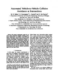
Fig. 1. The relative motion towards collision between camera/vehicle and target vehicles on straight and curved road. The self-vehicle has speed V0 and target vehicle has speed V1 . Left column is the vehicle and target positions in the world coordinate system and right column is the camera centered coordinate system to see relative motion of targets. Red circles are the potential collision positions.
The motion profile summarizes objects and, inherently, blurs small details. This generates dense flow as strong evidence of targets, since linear features are stable as compared to corner points with rich occlusion in driving video. Only vehicles, object rims, and road edges become visible in the motion profile. Another benefit of condensing is to reduce image to one dimensional data for fast computation. The extraction of potential collision from zero-flow also ignores most background and non-danger vehicles at early stage [12]. At the same time, the horizontal orientation in the entire view is divided to many zones. In the zero-flow zones, the color is further condensed (averaged) horizontally for examining the vertical motion. Based on that, convergence/divergence factor is computed from clusters of motion trajectories to confirm approaching vehicles, exclude leaving vehicles, and follow the vehicles moving in parallel. The T T C is thus obtained for collision alarming. In the following sections, we describe our motion data collection in Section III for zero-flow with possible danger. Section IV is to confirm flow divergence for alarming. Section V compute the Time-to-collision supported by Experiment in Section VI. II. P OTENTIAL C OLLISION AND A LERT S CENARIOS A. Potential Collision on Road The collision of a vehicle with other targets on road can be in different directions. To the camera mounted under the windshield of vehicle, such a collision has a relative velocity toward the camera as shown in Fig 1. The relative motion vector is aligning with a line of sight of the camera causing a zero-flow in the video. Even if a target moves on one line of sight, it may move away from the camera, stay at the same distance, and approach toward the camera with a potential collision. These actions will show the target size
(c) Fig. 2. Possible collision on different types of roads with relative motion between vehicles. Pink regions show the camera field of view. (a) Straight road and crossing road, with side lane vehicle cutting in, or front vehicle slowing down. (b) Curved road with opposite vehicle upcoming. (c) Merging road with collision danger.
reduced, stays the same, and enlarged, respectively. In the real environments shown in Fig. 2, such collision can happen with front target vehicle on straight road, merging vehicle on highway ramp, upcoming vehicle on curved road, crossing vehicle at intersection, etc. The Time-to-Collision (T T C) with the target is the distance between two vehicles divided by their relative speed. In the video, the T T C can be computed from the target size in the image divided by the size change during a short period, which will be proved in the following section. B. Precaution Scenarios In addition to potential collision, another set of scenarios are required to pay attention. This is the case that the relative motion of targets intersects the heading direction of camera, rather than directly towards the camera. Although it does not imply immediate collision, it may switch to a potential collision at next moment. As shown in examples in Fig. 3, the cut-in target vehicle from side lane may cause a collision if the target slows down further. On a curved road, the front vehicle slows down. Upcoming vehicle approaches. At an interaction, crossing targets move towards the vehicle heading direction. At a merging road, a vehicle speeds up from side without yield. These actions of target vehicles can be summarized in Fig. 4, where the relative motion vectors of target vehicles are toward the heading line of the camera/vehicle. These velocity vectors in the video frame are accompanied with a horizontal flow towards the Focus of Expansion (FOE), which is the penetrating point of camera translating direction with the image plane. If the relative target motion goes behind the camera, the camera/vehicle passes first without danger. An outgoing flow to a side appears on the target in the video. C. Vehicle Borne Camera and TTC After a camera is mounted on vehicle in the forward direction, its forward translation direction is determined by the vehicle and will not change during its driving on a straight
3
Straight road
Curved road
Merge road
Crossing road
Zero flow
Centered flow
Zero flow
Centered flow
Fig. 3. Different road collision cases cause horizontal motion and vertical flow expansion. The red arrows indicate motion direction of potential collision, green arrows mean safe motion, and orange arrows mean centered motion direction requiring attention. The vehicle heading direction is at the image center.
heading
Curved Upcoming Crossing
Merging yield vehicle
passed vehicle
Fig. 4. Some precaution cases where target vehicles generate centered flow in the video. (left) Actions on different roads: crossing, merging, upcoming and slow down with respect to the translation and rotation of camera on a curved road. (right) Relative motion that needs alert. If the extension of motion vector intersects the camera/vehicle heading direction (orange), it is a precaution case. If the extension is toward the back of camera (green), the image flow is outgoing in video and no collision will happen.
path. The FOE is thus fixed at a position in the video. Because our camera is set at a height lower than all the vehicle tops, the horizontal plane through the camera focus passes all the vehicles (lower than all the vehicle tops). If the vehicle is moving on a horizontal plane, the FOE is on the horizon projected in the image. In the video, the projected horizon cuts all the vehicles running on the same plane as the self-vehicle. We set the camera coordinate aligned with the vehicle, i.e., Z axis on the heading direction and the x axis with the horizon in the image. The image in video is denoted as I(x, y, t), where t is frame number, and the image flow vector or image velocity at point (x, y) is denoted as (u, v). The zero-flow for potential collision is described by u = 0 and the centered flow for alert can be described by u ∗ x < 0. The outgoing flow in the frame can be described by u ∗ x > 0, which is on passing target without danger of collision. If the vehicle/camera moves along a straight path, the points on background and vehicles moving in parallel toward the camera. A point passes line Z = 0 at the Time-to-Pass (T T P ). In such cases, T T P can be computed as T T P = x/u, where u is the derivative of x, i.e., horizontal image velocity.
For the points moving in a direction different from Z axis, e.g., a vehicle moving in its own direction on a curved road, above formula does not apply. It is not difficult to prove that 0 T T P for an object can be computed by T T P = D/D for all target moving directions, where D is the object size D = 0 x2 − x1 in the image, and D0 is the size change D = u2 − u1 in the video [10]. For a short proof, the perspective projection of camera is Xf X1 f X2 f x= , x1 = ,x2 = (1) Z Z Z Target width at the same depth (e.g., vehicle frontal or back surface) is ∆X = X1 − X2 6= 0, (2) and it is reflected to the image width ∆x according to (1) as ∆X =
(x1 − x2 )Z (∆x)Z x1 Z − x2 Z = = , f f f
(3)
The target width is constant during its approaching. Therefore, 0
0
∆X = 0,
0
∆x Z − ∆xZ =0 f
(4)
from (3). Thus, we have Z ∆x D = = 0 (5) Z0 ∆x0 D This means that the T T C computation is not related to camera property like focal length, but a precise time counting of target size in the video. All types of camera can implement this task. On the other hand, at least two lines are necessary to be paired on the same object in order to measure the object size. Only the motion with zero-flow may cause the collision, which yields real T T C. However, it is not easy to couple two vertical lines on an object without target recognition. This work does not attempt to perform whole frame vehicle or object recognition such that the proposed method will be more robust on general road environments. We rely on lines appearing horizontally and vertically in the video frame, and TTC =
4
y
t
P5
P3
P1
P0
P2
P4
Averaging verticallly in red belt
t
P6
x x (a) (b) Fig. 6. Computing target flow from the orientation of target trajectories in the motion profile. Color from green, red, to blue indicates positive, zero, and negative flow on the traces towards right, vertical, and left respectively.
x Fig. 5. One example of horizontal motion profile with motion trajectories of front targets. (top) Setting a sampling belt marked in red at the horizon in the frame. (bottom) Motion profile. Pi ’s are vertical motion profile zones.
response to the potential collision directly. Driving environments are full of lines, which can be categorized mainly in three types in video frames: (1) Horizontal lines on rear side of vehicle such as bumper, window, and top, shadow and road marks on the ground; (2) Vertical lines on vehicles and background such as poles, and side objects; and (3) Lines through depth on vehicle side view and adjacent lane marks. These lines are more continuous and robust to follow in video than points in the moving scenes. The size change of targets and background can be viewed as the convergence and divergence of motion flows of these lines in the video. III. M OTION P ROFILING TO C APTURE O BJECT MOTION A. Vertical Lines for Understanding Horizontal Movement To acquire vertical lines in the environment, multiple horizontal belts are placed near the horizon in each frame for vertical color condensing. Pixels in the belt are averaged vertically to produce a pixel line. Lines from consecutive frames are connected along the time axis to form a spatialtemporal image called Motion Profiles P (x, t) as in Fig. 5. Vertical features in video appear as trajectories in P (x, t).
The main advantage of motion profile is to ignore most of the background objects. The vehicles on road are guaranteed to be covered by the sampling belt because the camera positioning is lower than the roof of most vehicles. The belt height can also tolerate small vehicle pitch changes to obtain smooth motion trajectories when the vehicle moves on uneven roads. Motion profile reflects both long and short vertical features, which increases density of motion traces. The direction of motion trajectory is computed from the gradient orientation that provides the image motion of objects. This motion computation is more stable than optical flow based on two consecutive frames. In addition, the optical flow assumptions on invariant lighting and motion smoothness between frames are frequently violated in driving videos. Even if the trace color changes smoothly in the profile, the trace direction will not change. We compute the trace orientation based on the first derivative in the motion profile. To avoid the noise from digital sampling of motion profile, we use large filters (9 × 9 pixels) in 5 degree interval for orientation. Horizontal image velocity u is computed from u = arctan(θ) where θ =
max
−85≤θ≤90
Gθ
(6)
This will fill the velocity direction of traces almost everywhere in the motion profile. To obtain flow as dense as possible for the motion at all orientation as shown in Fig. 6, we lower down a threshold for picking meaningful gradient values as G(x, t)
|Gθ | > δ1
(7)
For those locations x with G(x, t) < δ1 , u is not reliable as noise. On the other hand, a temporal illumination change can occur when a vehicle goes under a shadow area. A large vehicle pitch may also cause abrupt color changes in the motion profile. These cause contrast edges orthogonal the time axis. Such edges are not real feature traces and are removed according to their close-to-horizontal orientation (u close to infinite) in the motion profile. Among all traces, a flow expansion along the time axis means object enlargement as its depth Z decreases.
5
t
an object robustly from color, parallelism, and coherence of traces in the horizontal motion profile. Therefore, we will not segment an object for its horizontal size, rather we examine the size changes vertically to identify approaching objects. These circumstances are summarized in Table I and are also illustrated in Figures 2 and 3. IV. V ERTICAL F LOW D IVERGENCE E STIMATION
x (a) (b) Fig. 7. Zero-flow locations shown in red color over a long period before (a) and after (b) median filtering.
B. Potential Collision in Motion Profile A potential collision of target toward the camera has a zeroflow in the video, which is a trace along the time axis. In a potential collision, Considering the physical size of the vehicle wider than the camera spot, the velocity slightly deviated from the line of sight may also cause collision to the body of selfvehicle. Thus, zero-flow region is defined as small flow as |u(x, t)| < δ2
(8)
which removes safe passing objects including vehicles, and instant changes of profile colors due to vehicle pitch/shaking and illumination changes. In addition to zero-flow, we pay attention to the flow towards image center (FOE). Thus, a non-zero-flow trace towards the image center (FOE) up to 80 degree in its orientation is included for attention, as long as it is constrained by u(x, t)x < 0. Rest of the flow directions indicates passing by objects without danger. This prevents further processing of non-collision objects and background in the video [12]. This processing may still contain digital errors. We further apply median filter in 9×9 regions to motion profile, u(x, t) to obtain reliable clusters of zero-flow regions. In details, in the homogeneous color regions obtained from (8) will produce discretized random noise due to insufficient time sampling of video on fast target motion. After median filter, the noise points are reduced as shown in Fig. 7. There are three cases in the horizontal zero-flow: target (1) approaching to, (2) leaving, and (3) keeping the same distance from the camera. Only approaching case will cause collision if no breaking or avoidance is taken. This can be confirmed from the flow divergence around the zero-flow spot, where an object is enlarged due to depth reducing. However, it is not reliable to segment the horizontal flow u(x, t) to individual objects from the motion differences, because (a) Multiple vehicles may have the same flow. (b) Complex occlusion between vehicles and background may not reveal entire objects. Flow at occluding point does not reflect true motion. (c) Background space between two target vehicles may expend or shrink in video, which is not the motion of a physical object. The flow divergence or convergence there does not imply a depth change of space. (d) Empty background, e.g., unpainted barrier has less feature on it. Overall, there is no guarantee on finding
Since neither target size nor depth are known under the horizon, the video frame is divided into vertical zones for further investigation. For simplicity, these zones are equal in size in order to compensate both straight and curved roads. The size is decided by considering the target scale at close and mid ranges. For example, the center zone that has the far distance is set approximately at the width of front or opposite vehicles 20m ahead. From these zones, a series of vertical motion profiles are obtained by condensing the color horizontally. In these vertical motion profiles, horizontal features on vehicle, crossing marks on the ground, and a part of road edges stretching in depth are strongly captured. Denote vertical zones as P0 , P1 , P2 , ..., Pn depicted in Fig. 5, with P0 at center, odd number zones on left and even number zones on right respectively. The scene convergence/divergence is determined in the zones. We compute the distinct flow in each profile where the zero-flow has been detected in order to measure the enlargement of objects in vertical profiles as in Fig. 8. Because of the scanning effect of side zones on the scenes sideways [13], the profiles may contain shapes of scenes rather than motion traces repeated by the same objects, if the zone does not have a zero-flow in the horizontal motion profile. Such scanned scenes provide no information on the object speed. We thus use the zero-flow weights obtained from the horizontal motion profile to limit the computation only on reliable vertical motion values. Figure 8 shows the pairs of horizontal and vertical profiles simultaneously obtained from video. Zero-flow regions are marked in horizontal profile P (x, t) and the vertical flow v is marked in the corresponding vertical profiles. The identified traces in the vertical profiles are mainly from horizontal features such as vehicle bumper, shadow, window, top, as well as from crossing road marks and shadows. Very slanted road edges in the image from a curved road or a merging road also respond to the condensing and leave trajectories in the vertical profiles, as summarized in Table I. Fortunately, only those horizontal lines supported by the approaching vertical lines on targets are examined for potential collision. Other horizontal lines are mostly road edges and surface lines that can be ignored here and pursued by other lane tracking modules. Finding the traces in a vertical profile can provide the speed information of targets relative to the camera in that direction. We also use oriented differential filters with 5 degree interval to pick the highest response as the vertical motion direction. The cost to obtain vertical profiles and computing flow are equivalent to averaging the entire image frame once, plus filtering in multiple orientations in y profiles. This is much smaller than the vehicle detection and recognition algorithms with a scalable window shifted in the field of view.
6
TABLE I A N OVERVIEW OF H ORIZONTAL AND V ERTICAL F EATURES IN M OTION P ROFILES AND T HEIR C LASSIFICATION BY DANGEROUS L EVELS . Flow
Size change
Zero-flow u=0 (potential collision)
Horizontal motion profile from Vertical Lines
Divergence u=0 Convergence
Vertical motion profile from Horizontal Lines
Centered flow (attention)
u>0, x0, x>0 u