Predicting Cloud Resource Utilization - Distributed Systems Group

Predicting Cloud Resource Utilization Michael Borkowski, Stefan Schulte, Christoph Hochreiner Distributed Systems Group TU Wien, Vienna, Austria

{m.borkowski, s.schulte, c.hochreiner}@infosys.tuwien.ac.at

ABSTRACT A major challenge in Cloud computing is resource provisioning for computational tasks. Not surprisingly, previous work has established a number of solutions to provide Cloud resources in an efficient manner. However, in order to realize a holistic resource provisioning model, a prediction of the future resource consumption of upcoming computational tasks is necessary. Nevertheless, the topic of prediction of Cloud resource utilization is still in its infancy stage. In this paper, we present an approach for predicting Cloud resource utilization on a per-task and per-resource level. For this, we apply machine learning-based prediction models. Based on extensive evaluation, we show that we can reduce the prediction error by 20 % in a typical case, and improvements above 89 % are among the best cases.

CCS Concepts •Information systems → Computing platforms; Enterprise information systems; •Computing methodologies → Neural networks;

Keywords Cloud computing; Resource usage; Usage prediction; Machine Learning

1.

INTRODUCTION

Resource provisioning and resource management are vivid fields of research in Cloud computing, resulting in a large number of according solutions [32]. Very often, the focus of resource management is on Quality of Service (QoS)-aware provisioning under given cost constraints, or under another set of rules [26]. Apart from a large number of general solutions for the Software-as-a-Service (SaaS) [31], Platform-asa-Service (PaaS) [1], and Infrastructure-as-a-Service (IaaS) [19] Cloud service models, more specific solutions exist, e.g., for the execution of scientific workflows [29], business processes [14], or data processing [12] in the Cloud. Permission to make digital or hard copies of all or part of this work for personal or classroom use is granted without fee provided that copies are not made or distributed for profit or commercial advantage and that copies bear this notice and the full citation on the first page. Copyrights for components of this work owned by others than ACM must be honored. Abstracting with credit is permitted. To copy otherwise, or republish, to post on servers or to redistribute to lists, requires prior specific permission and/or a fee. Request permissions from [email protected].

UCC ’16, December 06-09, 2016, Shanghai, China c 2016 ACM. ISBN 978-1-4503-4616-0/16/12. . . $15.00

DOI: http://dx.doi.org/10.1145/2996890.2996907

Resource provisioning involves dynamic allocation by scaling resources up and down depending on the current and future demand. While the individual aims of Cloud resource provisioning solutions differ quite a lot, e.g., taking into account QoS and Service Level Agreements (SLAs) [26], the basic approach is rather homogeneous: The goal is to distribute task requests onto Cloud-based computational resources, e.g., Virtual Machines (VMs) or containers [15]. Aside from deciding when to scale up or down, a common challenge is to distribute computational tasks across available computational resources. Resource provisioning approaches can be categorized into predictive and reactive strategies [8]. Reactive approaches measure a system’s state, e.g., the utilization of a VM, consider current task requests, and take according actions. In contrast, predictive approaches aim to predict the future behavior of the system. For instance, based on the number of user requests or data packages to be processed, the necessary amount of resources for a future period in time is calculated. Subsequently, Cloud resources are leased (or released) based on the predicted resource requirements, and tasks are distributed among these resources. These predictive approaches can lead to better resource efficiency and overall response time for the system, since they are able to adopt to system load in advance, instead of merely reacting in an ad hoc manner [16]. Despite the varying goals of the different predictive resource provisioning strategies presented in the literature, one common requirement of all of these approaches is a precise prediction about how many resources are actually needed to execute the computational tasks. Despite this fundamental requirement, to the best of our knowledge, surprisingly little research has been done so far in the field of prediction mechanisms for Cloud resource utilization. In order to address this challenge for efficient resource provisioning, we present a generic approach to predict Cloud resource utilization and task duration. We apply machine learning approaches to predict these values on a per-task level, based on historical task execution data. To this end, the remainder of this paper is structured as follows: In Section 2, we briefly discuss machine learning and describe our approach to resource utilization prediction. In Section 3, we present the experimental setup used to evaluate the proposed methods. The results of the evaluation are shown and discussed in Section 4. In Section 5, we discuss the related work in the field of prediction of Cloud resource utilization. Finally, we conclude our work in Section 6 and give an outlook on future work.

2.

MACHINE LEARNING APPROACH

For predicting resource utilization in the Cloud, we propose the employment of techniques from the field of machine learning. The intuition behind this is that tasks executed on Cloud-based computational resources often do not scale linearly with the cardinality of their input; therefore, the application of simple linear regression models is not sufficient. Furthermore, a task might take a vector of input data instead of a single item, making it necessary to perform multiple linear regression. Therefore, we propose to use machine learning in order to create prediction models from historic data, i.e., past task executions, and extract a model for obtaining future predictions.

2.1

Fundamentals of Machine Learning

Machine learning evolved from the study of pattern recognition and aims at giving computers the ability to decide problems without being explicitly programmed. Among the most popular machine learning approaches are Artificial Neural Network (ANN) models, which are inspired by biological neurons [4]. Such a network consists of artificial neurons, which have a certain number of inputs and an activation function. Its output can be used by other neurons as input. While choosing a machine learning model, we took into consideration the fair amount of research in the various areas. Compared to models suitable for classification like Bayesian classification [4] or Fisher’s linear discriminant [2] as well as regression models like Support Vector Machines, feed-forward ANN models with error backpropagation are well-suited for regression and provide efficient means of statistical pattern recognition [4, 11]. When the actual output for the given input vector is known, an error between the calculated and the actual output is calculated and used for training the model. In our case, this happens through backpropagation [11], which enables us to use compact models with sufficient generalization performance [4]. Machine learning distinguishes between offline and online learning: Offline learning occurs when all instances are presented simultaneously, while in the case of online learning, problem instances are presented one at a time [18]. In our instance, we perform offline learning, as training the ANN model involves processing large amounts of data, thus requiring a high amount of processing power. Furthermore, we employ supervised learning, i.e., we assume that for each instance of training data, the correct output is known and can be used for backpropagation.

2.2

Generic Architecture

As outlined in Section 1, resource provisioning is a common issue when Cloud-based computational resources are used. Usually, a task scheduler or provisioning agent is used to perform the leasing or releasing of the resources. In our architecture, a client, i.e., a consumer of Cloud services posts a request for the execution of a task to the provisioning agent. The provisioning agent is composed of the scheduler, which is responsible for performing task scheduling and provisioning, and the predictor, which supports the scheduler by predicting resource utilization. This enables the scheduler to optimize its decisions. Upon receiving a task execution request from the client, the provisioning agent must decide on how to provision Cloud resources. In current approaches, this means finding a schedule (time) and selecting computational resources (placement)

for the submitted task [13]. Such a decision requires knowledge about the duration and resource consumption of the task. For this, the scheduler queries the predictor to achieve a prediction of those metrics. Finally, after the execution, the Cloud infrastructure reports the actual resource usage back to the predictor. Recorded traces of this data, i.e., a history of predicted and actual resource utilization values, are then used by the predictor component to train its model.

2.3

System Model

In order to formalize our approach, we define the problem of predicting the resource usage for a given task to be provisioned. We assume that the provisioning agent has the following information about the task: • The type of task to be provisioned (T ) • A vector (a, b, c, ..., z) of input data for task T Furthermore, known a priori is a list of resources for which utilization is to be predicted. These resources are denoted as R1 , R2 , ..., Rn and can represent CPU time/cores, execution duration (time), memory usage, storage, or any other form of resource necessary to execute task T . c1 , R c2 , ..., R cn ), The result of a prediction is a vector (R c where Ri is the resource usage prediction for resource Ri .

2.4

Application to Resource Prediction

We propose to apply the presented machine learning approach to solve the resource utilization prediction problem described in Section 1. To this end, a prediction model Tb is created for the resource usage of every task T that requires such a prediction. The predicted resource usage then allows for an optimized provisioning. As discussed in Section 2.1, amongst machine learning methodologies, ANN models are the best fit for this purpose. Executions of a task T with an input vector (a, b, c, ..., z) produce a measured resource usage (R1 , R2 , ..., Rn ). This actual resource usage is recorded and used as training data. With an increasing amount of training data, the machine learning model becomes more and more fit, and therefore its predictions show increasing accuracy. After training, the model is able to predict the resource usage vector to a certain degree. In other words, the model can then be presented with a task T and an input vector (a, b, c, ..., z), and produces a resulting prediction vecc1 , R c2 , ..., R cn ). tor (R

3.

EXPERIMENTAL SETUP

As a proof of concept, the proposed machine learning approach has been thoroughly evaluated, based on an extensive set of experiments. In our evaluation, we aim to predict the duration of Cloud-based task executions as target variables. In other words, we model the duration a task requires as the b resource (R), and create a predictor function R. In the following subsections, we will introduce the applied metrics as well as the baseline against which we evaluate our prediction approach (Section 3.1), the test collection used for the experimentation (Section 3.2), the evaluation methodology (Section 3.3), the applied prediction approach (Section 3.4), and finally its implementation (Section 3.5).

3.1

Baseline & Metrics

In order to determine the degree to which machine learning improves the prediction of resource usage, we require a suitable baseline. In the literature, various approaches to predicting this usage exist, as we discuss in detail in Section 5. To establish a proper common ground for comparison, we have identified simple linear regression as a common element of these approaches. We have therefore implemented a basic linear regression predictor and compare our results against this baseline approach. In order to evaluate the accuracy of the proposed prediction model, it is necessary to observe differences between the b and the actual task duration R. For this, we prediction R apply the root-mean-square deviation (RMSD), a commonly used metric for evaluating the quality of predictions [17]. For a prediction model M and a set of test data T , the RMSD is defined as follows: sP RMSD(M ) =

t ∈ T (R(t)

2 b − R(t))

|T |

RMSDML RMSDB

(1)

(2)

Therefore, an error ratio of 1.0 designates that the machine learning approach achieved the same result as the baseline approach. Any error ratio > 1.0 indicates that the machine learning approach performs worse than the baseline, and a value < 1.0 indicates that the machine learning approach yields a lower RMSD than the baseline, thus performing better. We use this metric to be able to compare deviations regardless of their magnitude and unit.

3.2

Evaluation Dataset

To evaluate the proposed prediction approach, we have chosen an extensive dataset from Travis CI1 and GitHub2 . Travis CI is a publicly available continuous integration (CI) service for projects hosted on GitHub. For instance, when a developer pushes new code to GitHub, the CI server will detect this change, and trigger a new build/test/package cycle at Travis CI. For projects without a payment plan, Travis CI provides information about this CI process openly and without restriction. This data includes, amongst others, the name of the project (repository) that has been built, tested and packaged, the commit ID and the build duration. We gathered the evaluation dataset by creating a crawler based on the Travis CI API to collect data about project builds (build process records). The crawler ran for a total time of one week. We combined the data with the GitHub commits’ file counts and total sizes in bytes. By using the aforementioned API, we collected a raw dataset of over 3 million Travis CI build process records from over 35,000 GitHub repositories. Out of these, we removed repositories no longer publicly available (most likely due to deletion). We furthermore did not analyze repositories which were larger than 1 2

https://travis-ci.org/ https://github.com/

< T = (Repository, Language), a = File Count, b = Size, R = Duration >

(3)

For training, the data is stripped of its actual duration R b is (called label in machine learning), and the prediction R b calculated. The error between R and R is then given to the models as training input (backpropagation). For evaluation, b are compared to the actual value R, as the prediction R described in Section 3.1.

3.3

We designate the RMSD of the baseline as RMSDB and the RMSD of our machine learning approach as RMSDML . Following this, we observe the impact of our approach, and define its error ratio as: error ratio =

200 MB, since our analysis required actually checking out the code, which was not practical above a certain size threshold. The sanitized dataset consists of over 1.1 million build process records from around 10,500 repositories. Summarizing, the effective dataset we use for training of our resource prediction approach consists of tuples with the following structure:

Methodology

We conducted different preliminary experiments in order to assess the influence of different features on the prediction accuracy. In particular, we evaluated if the programming language of a repository alone would provide a sufficient level of prediction performance. This way, new repositories could be assessed using the existing machine learning model. This would allow tasks which are not yet known to the estimator to be handled without an initial learning phase. However, our initial analysis showed that aggregating builds per language, i.e., from many repositories, drastically reduces prediction accuracy. In our experiments, the median error ratio was around 800, which means that the machine learning approach had an error 800 times as large as the baseline approach. We therefore conclude that using perlanguage machine learning models is not feasible. For our approach, we therefore split the dataset by repository. In other words, we train one machine learning model per repository, instead of training one per language, or even a global one. This seems intuitive provided that our initial experiments have shown that individual repositories have very different build strategies. When generalized away from a CI task towards a generic Cloud computing platform, this step corresponds to training one machine learning model per scheduled task type, instead of training one global model. Finally, we grouped the build process records by repositories and split them into training and testing sets, with a split ratio of 70 % and 30 %, respectively.

3.4

Applied Prediction

As mentioned in the last section, we built one machine learning model for each repository. We therefore regard the repository as the task requiring execution (denoted as T in Section 2.3). Furthermore, we identified two parameters which might influence the build task: the amount of files in the repository at the time of the build, as well as the total repository size in bytes. Finally, the variable we want to predict is the duration of the task. We therefore formulate the following formal problem: For each task, the input variables are the repository itself (T ), as well as the file count (a) and the total size (b) of the repository. The variable to predict is the task duration (R). An overview of these variables is given in Table 1. Although ANN models generally accept the entire set of real numbers and thus the input domain of an ANN is not

Table 1: Machine Learning Model Variables T a b R

Variable Repository File Count Total Size Build Duration

Class Nominal Numeral Numeral Numeral

Type In In In Out

Example jlord/git-it 113 files 82 kB 32.8 s

Input Layer

Hidden Layer

Output Layer

2 Neurons

10 Neurons

1 Neuron

File Count Duration Total Size

limited, numbers around zero with a standard deviation of one are commonly used [3]. This is due to the fact that activation functions used in most ANN models operate in this region. This process is called normalization and has been shown to greatly improve prediction performance and reduce training time [27]. We therefore perform normalization by measuring the mean (µ) and standard deviation (σ) of the input training set, and then use linear normalization , in order to achieve this distribution. in the form of x−µ σ

3.5

Implementation and Configuration

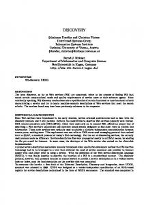
For the ANN implementation, we chose the open-source Java library Deeplearning4j (DL4J)3 , which provides machine learning capabilities. DL4J provides, amongst others, built-in support for multi-layer ANN models. We chose this kind of network due to its universal applicability [24]. While conducting research in order to obtain a set of parameters for the ANN, we found that using an ANN with a single hidden layer is suitable for most scenarios, including curve fitting, which our use case represents [24]. We furthermore found that using Stochastic Gradient Descent (SGD) [5] together with Nesterov’s Accelerated Gradient (NAG) [22, 23] is an established weight update method [28]. Furthermore, Glorot and Bengio [10] suggest using the Xavier weight initialization algorithm together with the tanh activation function. All of the selected algorithms are supported natively by DL4J. Table 2 summarizes the configuration of our ANN model. In Figure 1, we show a graphical representation of the network. An input vector is presented to the two input neurons, which produce an output according to their weights. This output is passed to 10 hidden layer neurons. The neurons in the hidden layer process their input values according to their weights, and their output is passed on to the output layer neuron. The output generated by this neuron is then accepted as the output of the network. In the training phase, the predicted resource utilization value obtained from the network output is compared to the actual (known) resource utilization. The error is then used to update the weights of the network according to the aforementioned update methodology. In the validation phase, the value obtained from the network output is also compared to the actual resource utilization, but the network is not updated, since it is already assumed to be trained. This is used to judge the network’s performance according the metrics described in Section 3.1.

4.

PERFORMANCE ANALYSIS

Based on the setting discussed in Section 3, we are able to perform evaluations of our prediction approach. We use the error ratio shown in (2) as an overall performance metric. To demonstrate the effects of machine learning, Figure 2 3

http://deeplearning4j.org/

.. .

Figure 1: ANN used for Evaluation Table 2: ANN Model Parameters Parameter Input Layer Neurons Hidden Layers Hidden Layer Neurons Output Layer Neurons Activation Function Learning Rate Minimization Algorithm Weight Initialization Weight Update Weight Update Momentum Training Epochs Iterations per Epoch

Value 2 1 10 per output 2 tanh 0.01 SGD [5] Xavier [10] NAG [22, 23] 0.9 250 1

shows the prediction performance of an examplary repository, which shows good training fit. The predicted duration is shown over the file count for the repository. Even though the fit is sometimes off by a constant value (biased), it performs reasonably well. Regarding the entire dataset, our main concern is naturally the distribution of instances with good fit and instances with bad fit in the results of our experiment. For this, we aggregated the error ratio values of all runs for the test data. We found that in the median case, the error ratio is 0.80 – in other words, our approach yields a 20 % decrease in prediction error. Furthermore, the error ratio of 1.0 or lower (i.e., the point until which our approach performs better than the baseline approach) has been reached for 72 % of all cases. This can be seen in detail in Table 3, which shows a summarizing view of the comparison of our approach against the baseline. We furthermore note that the performance in terms of learning duration, i.e., how fast the model could be trained, was not in the scope of this research. However, the results were obtained in about 30 s, using commodity hardware. While we used a particular test dataset for our experimenTable 3: Summary of Results Approach (Percentile) Baseline Machine Learning (worst 5 %) Machine Learning (median) Machine Learning (best 5 %)

RMSD 10.4 s 23.9 s 8.3 s 1.1 s

Error Ratio 1.00 2.30 0.80 0.11

3 000

Duration [s]

2 500

2 000

1 500

1 000

500 400 Training

450

500 File Count

Validation

550

600

650

Learning Results

Figure 2: Exemplary Training Results: Duration over File Count (Error Ratio = 0.267)

tation and evaluation, we nevertheless argue that the evaluation results are generally applicable. The dataset stems from a typical Cloud-based application, and the build processes used as example tasks within this paper are typical Cloud-based tasks – Cloud resources (in this case, time) are served to clients in an ad hoc manner. Nevertheless, using different test datasets, e.g., for stream processing, business processes or container instantiation, would yield significant results and are likely to confirm the applicability of our approach. Limitations of our approach consist mainly in the fact that in order to use a machine learning prediction model, sufficient training data is necessary. While we achieved satisfactory performance using even little training data, it is naturally not possible to infer any estimation without training. Furthermore, the computation power necessary to train a machine learning prediction model is non-negligible. When applying machine learning to applications with a large amount of resource prediction variables, special care must be taken not to cause too much prediction overhead. This could potentially outweigh the cost savings stemming from cost and time reduction of optimized resource provisioning and scheduling algorithms.

5.

RELATED WORK

Several approaches exist to predict or estimate the usage of resources for tasks to be provisioned using Cloudbased computational resources, ranging from relatively simple mechanisms to complex ones. In this section, we present and briefly discuss these approaches. [9] uses a hybrid approach of predictive and reactive provisioning, where the predictive approach works at coarse time scales (hours) and the reactive approach handles short-term peaks. [25] also uses historic data analysis, but employs a clone detection technique to determine whether resource access patterns have been encountered before. Similarly, [6] uses time series analysis and proposes an auto-scaling algorithm. However, for [6]. [9], and [25] no machine learning approaches are used. Similarly to the provisioning or placement problem, the scaling decision problem is the research area of a lot of

research, especially in Cloud computing. [6], [7], and [21] cover this subject, which is often done using machine learning techniques However, as argued in the introduction, the scaling decision problem (leasing and releasing) alone is often not sufficient for efficient operation. [30] is similar to our work in that it employs neuron-based systems to predict resource utilization behavior, but focuses on the clustering and load distribution of this prediction, instead of the prediction of resource utilization of tasks themselves. The paper uses load traces from 1997 to evaluate the approach. Islam et al. [16] propose empirical prediction of resource usage in the Cloud. For this, the authors apply ANN models and linear regression and analyze TPC-W, a specification for benchmarking e-commerce scalability and capacity planning for non-Cloud e-commerce websites [20]. While we focus on the prediction of per-task duration of different tasks, Islam et al. restrict the prediction to the overall CPU utilization. Thus, the results are more coarse-grained than in our approach. Finally, our work uses real-world data records instead of benchmarking for evaluation. Nevertheless, the work by Islam et al. comes closest to the work at hand.

6.

CONCLUSIONS

In Cloud computing, a predominant challenge is the provisioning of resources. Cloud service providers face the complex task of assigning client requests to their Cloud infrastructure. In current literature, the prediction of resource usage required to refine the provisioning strategy is often done using simple linear regression or fixed values. We propose using methods from the field of machine learning to build prediction models from historic data. Using a realworld dataset, we evaluate our approach and show that it indeed increases accuracy, compared to a simple linear regression approach. In the median case, our model predicted the duration of Cloud tasks with an error ratio of 0.80 (i.e., 20 % less prediction error). In the best 5 % of cases, an error ratio of 0.11 has been achieved (i.e., 89 % less prediction error). The main aim of our future work is to refine the applied prediction techniques. We expect improvement of the performance by using more sophisticated models like recurrent ANN. Furthermore, we would like to apply our approach to online learning scenarios; the current approach lacks renormalization techniques to balance out the neuron weights with new data. Finally, we currently only support fully supervised learning, where the actual resource utilization is known. Especially in initial stages of a learning model, usability would drastically improve if we could employ semisupervised or non-supervised learning.

Acknowledgment This work is partially supported by the Commission of the European Union within the CREMA H2020-RIA project (Grant agreement no. 637066) and by TU Wien research funds.

7.

REFERENCES

[1] L. Agostinho, G. Feliciano, L. Olivi, E. Cardozo, and E. Guimar˜ aes. A Bio-inspired Approach to Provisioning of Virtual Resources in Federated

[2] [3] [4]

[5]

[6]

[7]

[8]

[9]

[10]

[11]

[12]

[13]

[14]

[15]

[16]

[17]

Clouds. In 9th Int. Conf. on Dependable, Autonomic and Secure Comp., pages 598–604. IEEE, 2011. T. W. Anderson. An introduction to multivariate statistical analysis. Wiley, 1962. C. M. Bishop. Neural networks for pattern recognition, volume 92. Oxford university press, 1995. C. M. Bishop. Pattern Recognition and Machine Learning (Information Science and Statistics). Springer-Verlag New York, Secaucus, NJ, USA, 2006. L. Bottou. Large-Scale Machine Learning with Stochastic Gradient Descent. In Int. Conf. on Comp. Statistics (COMPSTAT), pages 177–186, 2010. E. Caron, F. Desprez, and A. Muresan. Forecasting for grid and cloud computing on-demand resources based on pattern matching. In Int. Conf. on Cloud Comp. Techn. and Science (CloudCom), pages 456–463, 2010. X. Dutreilh, S. Kirgizov, O. Melekhova, J. Malenfant, N. Rivierre, and I. Truck. Using reinforcement learning for autonomic resource allocation in clouds: towards a fully automated workflow. In Int. Conf. on Autonomic and Autonomous Systems (ICAS), pages 67–74, 2011. G. Galante and L. C. E. de Bona. A Survey on Cloud Computing Elasticity. In Int. Conf. on Utility and Cloud Comp., pages 263–270. IEEE, 2012. A. Gandhi, Y. Chen, D. Gmach, M. Arlitt, and M. Marwah. Hybrid resource provisioning for minimizing data center SLA violations and power consumption. Sustainable Comp.: Informatics and Systems, 2(2):91–104, 2012. X. Glorot and Y. Bengio. Understanding the difficulty of training deep feedforward neural networks. In Int. Conf. on Artificial Intelligence and Statistics (AISTATS), volume 9, pages 249–256, 2010. R. Hecht-Nielsen. Theory of the Backpropagation Neural Network. Int. Joint Conf. On Neural Networks (IJCNN), 1:593–605, 1989. C. Hochreiner, M. V¨ ogler, S. Schulte, and S. Dustdar. Elastic Stream Processing for the Internet of Things. In Int. Conf. on Cloud Comp. (CLOUD), pages 100–107. IEEE, 2016. P. Hoenisch, C. Hochreiner, D. Schuller, S. Schulte, J. Mendling, and S. Dustdar. Cost-Efficient Scheduling of Elastic Processes in Hybrid Clouds. In Int. Conf. on Cloud Comp. (CLOUD), pages 17–24, 2015. P. Hoenisch, D. Schuller, S. Schulte, C. Hochreiner, and S. Dustdar. Optimization of Complex Elastic Processes. Tran. on Services Comp., 2016. P. Hoenisch, I. Weber, S. Schulte, L. Zhu, and A. Fekete. Four-fold Auto-Scaling on a Contemporary Deployment Platform using Docker Containers. In Int. Conf. on Service Oriented Comp. (ICSOC), volume 9435 of Lecture Notes on Computer Science, pages 316–323. Springer, Heidelberg Berlin, 2015. S. Islam, J. Keung, K. Lee, and A. Liu. Empirical prediction models for adaptive resource provisioning in the cloud. Future Gen. Comp. Sys., 28(1):155–162, 2012. R. Jain. The art of computer systems performance

[18] [19]

[20] [21]

[22]

[23]

[24] [25]

[26]

[27]

[28]

[29]

[30]

[31]

[32]

analysis: techniques for experimental design, measurement, simulation, and modeling. Wiley, 1990. P. Langley. Elements of machine learning. Morgan Kaufmann, 1996. P. Leitner, W. Hummer, B. Satzger, C. Inzinger, and S. Dustdar. Cost-Efficient and Application SLA-Aware Client Side Request Scheduling in an Infrastructure-as-a-Service Cloud. In Int. Conf. on Cloud Comp. (CLOUD), pages 213–220. IEEE, 2012. D. A. Menasc´e. TPC-W: A benchmark for e-commerce. Internet Comp., 6(3):83–87, 2002. C. Napoli, G. Pappalardo, and E. Tramontana. A hybrid neuro–wavelet predictor for qos control and stability. In Cong. of the Italian Association for Artificial Intelligence, pages 527–538. Springer, 2013. Y. Nesterov. A method of solving a convex programming problem with convergence rate o (1/k2). In Soviet Mathematics Doklady, volume 27, pages 372–376, 1983. Y. Nesterov. Introductory Lectures on Convex Optimization: A Basic Course, volume 87. Springer Science & Business Media, 2003. R. Rojas. Neural networks: a systematic introduction. Springer Science & Business Media, 2013. M. Sarkar, T. Mondal, S. Roy, and N. Mukherjee. Resource requirement prediction using clone detection technique. Future Gen. Comp. Sys., 29(4):936–952, 2013. S. Singh and I. Chana. QoS-Aware Autonomic Resource Management in Cloud Computing: A Systematic Review. Comp. Surveys (CSUR), 48(3), 2016. J. Sola and J. Sevilla. Importance of input data normalization for the application of neural networks to complex industrial problems. Trans. on Nuclear Science, 44(3/3):1464–1468, 1997. I. Sutskever, J. Martens, G. Dahl, and G. Hinton. On the importance of initialization and momentum in deep learning. In Int. Conf. on Machine Learning (ICML), pages 1139–1147, 2013. C. Szabo and T. Kroeger. Evolving Multi-objective Strategies for Task Allocation of Scientific Workflows on Public Clouds. In Cong. on Evolutionary Comp. (CEC), pages 1–8. IEEE, 2012. C. Viswanath and C. Valliyammai. Cpu load prediction using anfis for grid computing. In Int. Conf. on Advances in Engineering, Science and Management (ICAESM), pages 343–348. IEEE, 2012. L. Wu, S. K. Garg, and R. Buyya. SLA-Based Resource Allocation for Software as a Service Provider (SaaS) in Cloud Computing Environments. In Int. Symp. on Cluster, Cloud and Grid Comp. (CCGrid), pages 195–204. IEEE, 2011. Z.-H. Zhan, X.-F. Liu, Y.-J. Gong, J. Zhang, H. S.-H. Chung, and Y. Li. Cloud Computing Resource Scheduling and a Survey of Its Evolutionary Approaches. Comp. Surveys (CSUR), 47(4), 2015.