Predicting Multiprocessor Memory Access Patterns with Learning ...

Proceedings of the Fourteenth International Conference on Machine Learning, ed. D. Fisher, Morgan Kaufmann, pp. 305-312, 1997

Predicting Multiprocessor Memory Access Patterns with Learning Models M.F. Sakr1,2, S. P. Levitan2, D. M. Chiarulli3, B. G. Horne1, C. L. Giles1,4 1NEC

Research Institute, Princeton, NJ, 08540 [email protected] 2EE Department, University of Pittsburgh, Pittsburgh, PA, 15261 3CS Department, University of Pittsburgh, Pittsburgh, PA, 15260 4UMIACS, University of Maryland, College Park, MD 20742 Abstract Machine learning techniques are applicable to computer system optimization. We show that shared memory multiprocessors can successfully utilize machine learning algorithms for memory access pattern prediction. In particular three different on-line machine learning prediction techniques were tested to learn and predict repetitive memory access patterns for three typical parallel processing applications, the 2-D relaxation algorithm, matrix multiply and Fast Fourier Transform on a shared memory multiprocessor. The predictions were then used by a routing control algorithm to reduce control latency in the interconnection network by configuring the interconnection network to provide needed memory access paths before they were requested. Three trainable prediction techniques were used and tested: 1). a Markov predictor, 2). a linear predictor and 3). a time delay neural network (TDNN) predictor. Different predictors performed best on different applications, but the TDNN produced uniformly good results.

1 INTRODUCTION Large scale multiprocessor systems require low-cost, highly-scalable, and dynamically reconfigurable interconnection networks (INs) (Siegel, 90). Such INs offer a limited number of communication channels that are configured on demand to satisfy required processor-memory accesses. In this demand driven environment, a processor accessing a memory module makes a request to an IN controller to establish a path (reconfigure the IN) that satisfies the processor’s request. The controller is used to optimize the required IN configuration based on the set of

Copyright Morgan Kaufmann

current processor requests. Hence, the end-to-end latency incurred by such INs can be characterized by three components (Figure 1): control time, which is the time needed to determine the new IN configuration and to physically establish the paths in the IN; launch time, the time to transmit the data into the IN; and fly time, the time needed for the message to travel through the IN to its final destination. Launch time can be reduced by using high bandwidth opto-electronic INs, and fly time is relatively insignificant in such an environment since the end-to-end distances are relatively short. Therefore, control time dominates the communication latency. However, in a multiprocessor system executing a parallel scientific application, the memory-access requests made by the processors follow a repetitive pattern based on the application. Compilers can analyze an application and attempt to predict its access patterns (Gornish, 90), but often the pattern is dynamic and thus hard to predict. The goal of this work is to employ a technique that learns these patterns on-line, predicts the processor requests, and performs the IN configuration prior to the requests being issued, thus hiding the control latency. The effect is a significant reduction in the communications latency for multiprocessor systems. Control

Launch

Fly

Lc

Ll

Lf

Time

Processor Request Figure 1: The three components of the end-to-end communication latency; control time, launch time and fly time. Control time dominates overall communication latency.

Learning methods have been applied in various areas of computing and communication systems. For instance, neural networks have been applied to learn both network topology and traffic patterns for routing and control of communication networks (Fritsch, 91), (Jensen, 90), (Thomopoulos, 91). Using neurocomputing in high speed communication networks was the subject of a special issue of Communications (Habib, 95). Also, using a neural network as a static branch prediction technique was recently presented by (Calder, 1997). Other applications of neural networks are for the control of switching elements of a multistage interconnection network for parallel computers (Funabiki, 93), (Giles, 95) and for learning the structure of interconnection networks (Goudreau, 95). For multicomputer systems, genetic algorithms have been applied as a distributed task scheduling technique (Wang, 95). Solutions to the problem of mapping parallel programs onto multicomputer systems to provide load balancing and minimize interprocessor communication have been proposed using genetic algorithms (Seredynski, 94) and self organizing maps (Dormans, 95) as well as variants of the Growing Cell Structures network (Tumuluri, 96). In uniprocessor environments, Stigal et. al. (Stigal, 91) propose a neural network cache replacement algorithm. Their technique predicts which cache block will be accessed furthest in the future and therefore should be replaced, thus lowering the cache miss rate. In general, the literature on machine learning in computing and communication systems has focused on how these techniques can be used to identify patterns of communication in order to optimize the control of these systems. The focus of this work is to study how three on-line learning methods perform at predicting processor-memory access patterns in a multiprocessor environment. We use a Markov predictor, a linear predictor and a timedelay neural network (TDNN) (Lang, 90) to learn and predict the memory access patterns of three parallelized scientific applications: a 2-D relaxation algorithm, a matrix multiply, and a 1-D FFT. The next section presents the environment of our experiment where we describe a shared memory multiprocessor model employing prediction units. In section 3, we describe the three prediction methods used and in section 4 we present experimental results of the predictors. The final section interprets our results and discusses future directions of research.

2 MULTIPROCESSOR MODELS Shared memory parallel computers are commonly referred to as multiprocessor systems (Bell, 85), (Kumar, 94). Our shared memory multiprocessor (SMM) system consists of 8 processors (P0-P7), 32 memory modules (M0-M31), a reconfigurable IN and an IN controller (Figure 2). This SMM model uses a state-sequence router (Chiarulli, 94) as the reconfigurable interconnection network controller. In addition, we use a SMM simulator which allows us to record the memory access traces of parallel applications.

IN Controller based on the State Sequence Routing Paradigm State Transformer

Faults

State Generator 1 P0-M3; P2-M14; P5-M7 2 P1-M3; P6-M5; P7-M4

Predictions k IN Configurations

P0 PU P1

M0

PU

Reconfigurable

M1

Interconnection Network (IN) P6 P7

PU PU

M30 M31

Figure 2: An 8✕32 shared memory multiprocessor system employing the SSR paradigm as the IN controller and one on-line Prediction Unit (PU) per processor. In such systems with N processors and K memory modules, the reconfigurable IN can be configured to achieve any of the N✕K possible paths between a processor and a memory module; however, it can only provide a subset of these paths at any given time. A group of compatible (nonblocking) paths are called an IN configuration or a state. Because of contention for paths, the IN must be dynamically reconfigured to satisfy the set of current processormemory accesses. This SMM model employs an IN control system based on the state sequence routing (SSR) paradigm (Chiarulli, 94) which takes advantage of the locality characteristics exhibited in memory access patterns (Johnson, 92) and reconfigures the network through a fixed set of configurations in a repetitive manner. The IN controller, used for state sequence routing, consists of a state generator which is controlled by a state transformer. The state generator maintains a collection of configurations, called a state sequence and periodically reconfigures the IN with a new configuration from the set. Specifically, the state sequence is maintained in a cyclic shift register of length k as shown in Figure 2. With each register shift, an IN configuration is broadcast to the processors, memory modules, and switching elements of the IN. The state sequence router exploits the memory access locality inherent in these patterns by re-using the sequence of states. The state transformer is responsible for determining the set of configurations contained within the state generator based on processor requests. A processor that needs to access a memory module issues a fault (or request) to the state transformer only if the current state sequence does not already include the required path to a memory module. In response, the state transformer adds the required path to the state sequence by removing the least recently used path.

Using SSR the average control latency, L, incurred by each access can be shown to be:

k L c = ( 1 – p ) --- + p ( k + f ) 2

(1)

where p is the probability of a fault, k is the sequence length, and f is the fault service time. If a processor needs a path and it exists in the state sequence, there is no fault issued and the latency is just the time for the path to come around in the sequence which on an average is k/2. However if the path does not exist after k broadcasts, the processor issues a fault which must be serviced before the memory access can occur. The SSR based IN controller needs only to establish the initial paths and respond to the changes in the memory access pattern; it is not required to respond to individual memory access requests. Our goal is to employ a technique that reduces the probability of a fault by predicting changes in memory access patterns and informing the controller of a needed transformation before a fault occurs. Thus, the controller will transform the state sequence to include the soon-to-beneeded path, avoiding the latency incurred by the fault. As shown in Figure 2, a prediction unit (PU) is used to learn the access pattern of each processor. The predictions made by the PU are used as hints by the SSR while routing the memory accesses. Since, processor-memory access patterns change dynamically and thus can be modeled as a time series, for this preliminary investigation, we chose to study three simple on-line time series prediction methods: a Markov predictor, a linear predictor and a TDNN.

3 PREDICTION METHOD EXPERIMENT To evaluate the performance of various prediction methods, we test how well each technique can predict the next memory access pattern as the SMM executes three typical parallelized scientific applications. The first application is a parallel (32✕32) 2-D grid-based temperature propagation/relaxation algorithm; the second application is a repetitive (24✕12 • 12✕24) matrix multiply program; the third is the memory access pattern generated from a repetitive 1D Fast Fourier Transform (FFT) of a 16 sample vector. Each experiment consists of three distinct phases: First, using the shared memory multiprocessor (SMM) simulator, we generate the memory accesses of a parallel program assuming fixed latency in the IN and memory modules. Using the raw memory accesses generated by the SMM simulator, we extract the sequence of memory accesses of a single processor. This memory access is represented differently depending on the predictor used. For each experiment we use the 32 memory module access pattern of a single processor, these patterns are shown in Figures 3a, 4a, and 5a. The applications are symmetrically partitioned to execute the same code on all processors while each processor uses different parts of the data. Hence, the access patterns of all other processors are very

similar to the one used. Second, we use the processor’s memory access patterns as input to the PU to perform online training and one-step ahead prediction of the next memory access. Third, we evaluate the predictions by simulating the multiprocessor behavior with and without the predictions and monitor the number of faults incurred. For each of the experiments we use a relatively short state sequence length (k). As can be seen from Equation 1, the optimum sequence length, k, is a trade off between increasing k to reduce faults, and keeping k small to reduce waiting time. The values of k were chosen to minimize the faults for these applications, for the non-predictive case. We tested using the best 1, 2, 3 and 4 predictions of the PUs as hints to the SSR controller. The three prediction methods tested are considered appropriate for this dynamic system since the training and prediction is performed on-line. 3.1 MARKOV PREDICTOR There are many ways one could consider using a Markov predictor (Isaacson, 76). We consider both a first and second order predictor which calculates the conditional probability p of accessing memory module Mi given processor Pk has just accessed memory module Mj, i.e. p(Mi|Mj;Pk). Similarly, for the second order, we calculate p(Mi|Mj,Mq;Pk) where the conditional probability is conditioned on processor Pk previously accessing memory module Mq, then Mj. Since in this model we use one PU per processor, the input of the Markov prediction unit is the temporal sequence depicting the memory access pattern of a processor. The probabilities are stored in a probability transition matrix. For the first order predictor, probability pij corresponds to the probability of accessing memory module i if the processor is currently accessing memory module j. Similarly for the second order predictor, pi(jq) corresponds to the probability of accessing memory module i if the processor is currently accessing memory module j after completing an access to memory module q. Each entry in the transition matrix is updated and normalized on-line as the application execution proceeds. For example, in the first order Markov predictor of processor P0, the probability of processor P0 going from M1 to M2 at time step t is calculated as the number of transitions P0 has performed from M1 to M2 divided by the total number of times P0 has accessed M1 from time 0 to time t. The number of parameters needed for the first order Markov predictor is 1024 probabilities while the number of parameters for the second order Markov is 32K probabilities. However, both first and second order predictors update 32 probabilities on-line with every access since the next access could go to one of 32 memory modules. At any given time, the non-zero probabilities are the predictions given to the state sequence router. However, the number of non-zero probabilities could be up to 32, therefore, a fixed number of the most likely predictions is specified. We tested the first and second order Markov predictors using the highest 1, 2, 3, and 4 probabilities as predictions. Also, we tested the system using state sequence lengths (k)

of size 4, 5, 6 and 7. The results for each access pattern are discussed in the results section and the best results are depicted in Figures 3c, 4c, and 5c. The performance of the Markov predictor is compared to that of the Linear and TDNN PUs in Section 4. 3.2 LINEAR PREDICTOR For the Linear PU, the input data is transformed from a processor’s raw 32 memory module traces into a sequence of 32 bit binary vectors. The ith component of the binary vector is set to 1 when an access to the ith memory module takes place. All other values in that vector are set to zero. For each value in the binary symbol vector we use a next step linear predictor which attempts to predict the next access based on a linear combination of all the values in the vector and their history. Since there are 32 memory modules (1✕32 access vector) in the system tested, we use 32 linear predictors that predict the next access vector in parallel. In order to compare the results of this predictor with that of the TDNN we use one bias weight for each output value, hence the Linear predictor is actually an affine predictor (Hecht, 91): l

xˆ ( t + 1 ) = i

32

∑∑

w

i=1,2,…32; l=1,5,10 (2) x (t – k )+ w ijk j i0

k=0j=1

where x is a binary vector of dimension 32, xi denotes the ith component and xˆ is the prediction. Since we are implementing one-step-ahead prediction, the Linear predictor takes as input the current binary vector and the past l history vectors and attempts to predict the vector x at the next time step (Equation 2). We tested the performance of the Linear predictor using l = 1, 5, and 10 past vectors. Therefore, the number of inputs for the three Linear predictors tested are 64, 192, 352 (32 × (l + 1)) and the number of coefficients (weights) to update at each time step is 2080, 6176, 11296 respectively. The learning algorithm is a simple on-line gradient descent algorithm using the following adaptive learning rate, starting value is set to 0.01: if ( (present error - previous error) > previous error × 10% ){ reduce learning rate by a decrease factor of 0.5 and move back in the weight space to the previous point} else { keep the updated weights and increase the learning rate by an increase factor of 1.1}

The algorithm is performed on-line, so we make only one pass through the data. Furthermore, the outputs (predictions) with values > 0.5 of which the largest values are selected as the predictions which are passed along to the state sequence router as hints. We tested using 1, 2, 3 or 4 predictions as hints to the SSR controller. The best results of the Linear predictor are depicted in Figures 3d, 4d, and 5d.

3.3 TIME DELAY NEURAL NETWORK The data encoding of the memory accesses for the TDNN is the same as that of the Linear predictor. Again, since we are implementing one-step-ahead prediction, the TDNN takes as input the current binary vector and attempts to predict the access vector at the next time step as in (Sakr, 96). Therefore there are 32 inputs and 32 outputs for the network. For each input, we experiment with a tapped delay line of length 1, 5 or 10. The total number of inputs to the multilayer perceptron (MLP) section of the TDNN is 64, 192, 352 derived from (32 ✕ (1 input + # taps)). We tested the performance of the TDNN using a single hidden layer of size 10, 20 and 30 neurons. Every output node has an additional bias weight, we use tapped delay lines of sizes 1, 5 and 10. This gives 1002, 2282, 3882 total weights for the TDNN with 10 nodes in the hidden layer; 1972, 4532, 7732 total weights for the TDNN with 20 nodes in the hidden layer; and 2942, 6782, 11582 total weights for the TDNN with 30 nodes in the hidden layer. Nodes in the hidden layer use a hyperbolic tangent activation function, while nodes in the output layer are affine. All of the weights were initialized uniformly in the range [-1/φ, 1/φ], where φ is the number of connections that enter a node (fan in). The learning algorithm is a simple on-line gradient descent algorithm using the same adaptive learning rate used for the Linear predictor. Since the training and prediction is performed on-line, we make only one pass through the data. Many prediction interpretations could be used; we found that best performance was achieved if the output neurons with the largest values are selected as predictions. We tested using 1, 2, 3 or 4 output neurons with the highest values as prediction hints to the SSR controller. The best performance of the TDNN is shown in Figures 3e, 4e, and 5e.

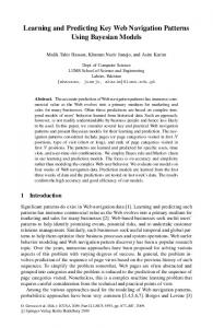
4 RESULTS In this section we discuss the performance of the three prediction units tested for the three applications implemented on our SMM model. In order to compare the performance of the prediction units, for each application we plot the memory access pattern followed by fault plots. First we show the characteristic access pattern of each of the applications in Figures 3a, 4a, and 5a. Then the network faults incurred for the non-predictive case (Figures 3b, 4b, and 5b) followed by the network faults incurred by the system using the PUs (Figures 3c-e, 4c-e, and 5ce). In this paper we report on the best results of each of the predictors for each application, across the space of the system and predictor parameters tested. For the complete results see (Sakr, 96b). 4.1 2-D RELAXATION Figure 3a shows 8697 access vectors which depict the access behavior of the 2-D Relaxation algorithm, the large discontinuity in the pattern is a no-memory-access period which is a characteristic of the algorithm. The

access patterns exhibit a stair-like behavior, where each stair discontinuity reflects a change in the memory module access. For this access pattern the first order Markov predictor performed the best of the three prediction units tested. The second order Markov predictor shows improved performance over the first order only for the 1 prediction case. In general, increasing the number of predictions used by the state sequence router enhanced performance while increasing the size of the state sequence (k) does not for this particular application. For the Linear predictor, increasing the history or the number of predic30

Memory Module

25

20

15

10

5

0 0

500000

1e+06

1.5e+06

2e+06

Time (a) Faults

4.2 MATRIX MULTIPLY (b) no PU

1.4

1.2

1

0.8

0.6

0.4

0.2

0 0

500000

1e+06

1.5e+06

2e+06

Time Faults

1.4

(c) Markov PU

1.2

1

0.8

0.6

0.4

0.2

0 0

500000

1e+06

1.5e+06

2e+06

Time Faults

1.4

(d) Linear PU

1.2

1

0.8

0.6

0.4

0.2

0 0

500000

1e+06

1.5e+06

2e+06

Time Faults

1.4

(e) TDNN PU

1.2

1

0.8

0.6

0.4

0.2

0 0

500000

1e+06

tions used as hints does not enhance performance. On the other hand, increasing k helps increase the total number of network faults eliminated. We tested many TDNN configurations, the performance of the TDNN in predicting this pattern relied heavily on the number of nodes in the hidden layer. Increasing the history used (tapped-delay line) does not improve performance as much as increasing the size of the hidden layer. Using a large k is also crucial in fault elimination for this pattern. Figure 3b plots the network faults incurred as impulses for the non-predictive case. The other fault plots show the best performance of the online predictors for the 2-D relaxation algorithm. The first order Markov predictor using 3 predictions and a k of size 3 eliminated 96% of the network faults. It performs best for this pattern since the total number of non-zero probabilities is small (three), and using the top three probabilities is enough to predict almost perfectly and eliminate all faults (Figure 3c). The best performance of the Linear predictor was achieved by using 1 past access vector, 2 predictions and a k of size 6 eliminating 95% of all faults. Compared to the Markov predictor, the Linear predictor needs a few more training iterations before its predictions start to greatly reduce the number of faults (Figure 3d). The TDNN with a hidden layer of 30 nodes, a tapped delay line of size 2 and k of size 7 produced its best result eliminating 71% of the network faults, shown in Figure 3e.

1.5e+06

2e+06

Time Figure 3: (a) The memory access pattern of the 2-D relaxation algorithm for Processor P0. (b) The number of network faults incurred without predictions. (c) Number of network faults using the Markov PU. (d) Number of network faults using the Linear PU. (e) Number of network faults using the TDNN PU.

The matrix multiply application exhibits a more complex pattern since each processor accesses the memory modules in a less uniform fashion than the 2-D relaxation algorithm. Figure 4a shows the 11561 vector access pattern. Since this application exhibits a complex access pattern the first and second order Markov predictors cannot capture and predict the access pattern correctly. Increasing the number of predictions or k does not enhance overall performance. The performance of the Linear predictor is similar to that of the Markov predictor for this application. Varying the history, or k, or the number of predictions does not improve performance. On the other hand, the TDNN produces marginally better results. The TDNN performs best with a hidden layer of 10 nodes, using 2 predictions and a k of size 7 achieving 30% fault reduction. However, increasing the size of the hidden layer hinders the performance of the TDNN. Figures 4b-e show the best performance of all three prediction units for this access pattern. In this case, the Markov predictor performs poorly since the probabilities are of equal values which increases the number of wrong predictions. Specifically, the second order Markov predictor using 4 predictions and a k of size 5 eliminated 6% of the faults. The best performance of the Linear predictor, eliminating 1% of the faults, was achieved using 10 past access vectors, 1prediction and a k of size 6. The linear predictor is not able to find a linear combination of the past accesses to predict the next access well. However, the TDNN still achieves a moderate reduction in the number of faults.

the percentage of fault elimination for both the first and second order Markov predictors. The Linear predictor produces its best results when using the least history, the least number of predictions and a k of size 6. Increasing the history used or the number of predictions does not boost performance. The TDNN is capable of learning and predicting the access pattern of the FFT. A hidden layer consisting of 10 nodes provides better performance than the TDNN with a larger hidden layer. A number of predic-

30

Memory Module

25

20

15

10

5

30

0 0

500000

1e+06

1.5e+06

25

2e+06

Faults

1.4

Memory Module

Time (a) (b) no PU

1.2

1

0.8

0.6

0.4

0.2

20

15

10

0 1.8e+06

1.9e+06

2e+06

2.1e+06

2.2e+06

2.3e+06

Time Faults

5

(c) Markov PU

1.4

1.2

1

0.8

0

0.6

0

20000

40000

60000

0.4

0 1.8e+06

1.9e+06

2e+06

2.1e+06

2.2e+06

2.3e+06

Time (d) Linear PU

1.2

100000

1

0.8

0.6

0.4

120000

140000

160000

(b) no PU

1.4

Faults

Faults

1.4

80000

Time (a)

0.2

1.2

1

0.8

0.6

0.2

0.4 0 1.8e+06

1.9e+06

2e+06

2.1e+06

2.2e+06

2.3e+06

0.2

Time 1.4

0

20000

40000

60000

80000

100000

120000

140000

160000

Time

(e) TDNN PU

1.4

Faults

1.2

Faults

0

1

0.8

0.6

0.4

0.2

(c) Markov PU

1.2

1

0.8

0.6

0.4

0 1.8e+06

1.9e+06

2e+06

2.1e+06

2.2e+06

0.2

2.3e+06

Time

0

20000

40000

60000

80000

100000

140000

160000

(d) Linear PU

1.4

1.2

1

0.8

0.6

0.4

0.2

0 0

20000

40000

60000

80000

100000

120000

140000

160000

Time Faults

1.4

4.3 FAST FOURIER TRANSFORM

120000

Time Faults

Figure 4: (a) The memory access pattern of the matrix multiply for Processor P0. (b) The number of network faults incurred without predictions. (c) Number of network faults using the Markov PU. (d) Number of network faults using the Linear PU. (e) Number of network faults using the TDNN PU.

0

(e) TDNN PU

1.2

1

0.8

0.6

0.4

0.2

The FFT application produces the memory access pattern shown in Figure 5a. The Markov predictor is capable of capturing and predicting this pattern thus eliminating almost all the faults incurred by the state sequence router. The second order Markov captures the pattern of access thus producing better results compared to the first order Markov. Increasing the number of predictions used is essential for good performance while increasing k does not affect

0 0

20000

40000

60000

80000

100000

120000

140000

160000

Time Figure 5: (a) The memory access pattern of the FFT for Processor P5. (b) The number of network faults incurred without predictions. (c) Number of network faults using the Markov PU. (d) Number of network faults using the Linear PU. (e) Number of network faults using the TDNN PU.

tions of either 2 or 3 with a k of size 6 or 7 are needed for good performance. Figures 5b-e show the best results of the PUs for this access pattern. Since the FFT algorithm exhibits a simple access pattern, the second order Markov predictor is able to capture the pattern and predict well eliminating 95% of the faults using the top four predictions and a k of size 4. The Linear predictor using 1 past access vector, 1 prediction and a k of size 6 is capable of eliminating some, 34%, of the network faults. The TDNN with 10 nodes in the hidden layer, a tapped delay line of size 10, using the top 2 predictions and a k of size 6 eliminated 45% of the faults. The TDNN performs better than the Linear predictor for this pattern but not better than the Markov.

5 SUMMARY AND CONCLUSIONS Completely connected interconnection networks (INs) are not feasible in large scale multiprocessor systems because of their high complexity and soaring cost. Accordingly, we utilize less expensive reconfigurable interconnection networks that scale well but suffer from high overhead due to control latency. Control latency is the time delay incurred by the network controller to determine a new desired IN configuration and to physically establish the paths in the network. Each reconfiguration request (network fault) is triggered when the current network configuration fails to satisfy a processor’s memory access. These requests are performed on a demand driven basis. However, memory access patterns of multiprocessor systems executing parallel scientific applications exhibit a lot of repetitiveness due to loops which are a characteristic of such applications. Hence, in this work we study how three learning methods perform at learning and predicting these access patterns on-line. Correct prediction of the access patterns allows anticipatory reconfiguration of the IN and thereby satisfy the forthcoming memory accesses preventing a network fault. Thus, the average control latency L is hidden and consequently overall communication latency is reduced. The three on-line prediction methods tested are: a first and a second order Markov predictor; a linear prediction method; and a time delay neural network (TDNN). We train the prediction methods using the access patterns of three parallel scientific applications: a 2D relaxation algorithm; a matrix multiply; and a Fast Fourier Transform (FFT). The multiprocessor model used is an 8 processor 32 memory module shared memory system with a state sequence router as the reconfigurable interconnection controller. The experiments show that coupling state sequence routing with different types of on-line prediction methods can decrease the number of memory access faults across different applications with some methods being more effective than others. The best results of the prediction methods for the access patterns tested are as follows (Table 1). For the 2D relaxation algorithm the first order Markov predictor eliminates 96% of the faults; the Linear predictor pre-

vents 95% of the faults; and the TDNN removes 71% of the faults. While for the matrix multiply: the second order Markov predictor eliminates 6% of the faults; the linear predictor removes 1% of the faults; and the TDNN prevents 30% of the network faults from taking place. Finally, using the access patterns of the FFT: the second order Markov predictor prevents 95% of the network faults; the linear predictor eliminates 34% of the faults; and the TDNN removes 45% of the network faults. As expected, different predictors perform best on different applications. From visual inspection of the access patterns (shown in Figures 3a, 4a, and 5a), one could say that the access patterns of different applications vary in complexity from the 2-D relaxation being the most simple to the matrix multiply the most complex. All prediction methods perform well on the applications with the simple access patterns. On the other hand, for very complex patterns, the Markov and Linear prediction methods perform very poorly and TDNN gives uniformly good results. Table 1: Percentage of faults eliminated for the three best learning techniques tested using the access patterns of three parallel applications Markov Predictor

Linear Predictor

TDNN Predictor

2-D Relaxation

96%

95%

71%

Matrix Multiply

6%

1%

30%

FFT

95%

34%

45%

Given the multiprocessing environment, different applications exhibit very different patterns and a technique that will predict well across patterns is more appealing than a technique that performs best for specific patterns. Thus, we hypothesize that the TDNN has the best chance of adapting to different memory access patterns from the variety of real applications. However, it could be feasible to use all prediction methods in a mixture of experts model (Jordan, 94) and use the best predictor available. Future work should address more realistic simulation of the multiprocessor environment, such as the effects of incorporating runtime delays due to memory and network contention in the memory access patterns and how these prediction methods affect actual performance. We plan to test the performance of different machine learning techniques and other prediction methods. Also, it would be interesting to investigate the applicability of prediction techniques to the general problem of latency hiding at all levels of the memory hierarchy. Another open question is how will these prediction methods be efficiently implemented in hardware and their results effectively used. For example how and what is the effect of memory fault prediction in the actual speedup of applications on a multiprocessor?

References



  
 "!# $% & '( )* +-, .  /01+-'( *2+304'5+ . / 06*798;:=?+- @
BAA7>//C
DE AF DEG
H
IJ) K 07MLN
IB06$%&) K7MO
IPQ+3$% 27ML>
IR$SK*)T57MP
U)06$%7VO
WU+-XY07[Z\H
W]^+30_$%7V  G *
W`=?K $%'5 F a )2 K *)' a 0_)$%'(b /01 K'5+-$ *$%c . )'5b%$%  )06$S$%c?8%
edMfSg hi6j(k?l6j(mnoqp(k?l p5k ri@p@s%i6j(tutuovk s w j(k s%x-j@s%y1lzj5k-{}|?~l6ny6tul677FAAA%
L>

SJb%)06  7^:
€-
SR =)$S7^‚}

SU b% . 7C
Sƒu)+  D *
„R+-'() T…)* K†J+3$%01+3 ‡#u c-+-0_b . ˆ,+30 ‚^ '(+-$%‰c?0_) a ‹ŠQ$% 01'(+-$%$% '5+-$ŒŽ &Ž+-06?*798dM‘‘’qoqy6{ “ ‘noqml17=+- @
*””7//C
*AF” G

SLu+30 . )$%27^•
FQ–>
•Ž 2> 
€)0_+-$%$%c„)$SK U)//$%c +-, R)01c? —?`UFB0_)/b% a T :p(i6ž5l1Ÿp5‘™p(k rj(i6j5’q’vy6’Cj(k?{¡ uovl6nQi6ov¢Yx-nQy1{¡ri@p5m_y6l6l6oqk s%7z:£)$„‚^+ .  +37¤ŠQ) T(7 //C
*AA G FA”%
¥
¦—?062'(b%7¨§4
¦U)$%K © Q
¦J+ .ª. $%'5)+-$ ŒŽ &Ž+-06«‚^+-$%c«–u*$%c«ŒY06) ¬ŒŽ 2FŒŽ .  06'5) #u*/ '5 )$%K #u  06$S)= #u//01+3)'5b% *798 ­Qššš ­k?ny6i6k?j(noqp(k?j(’¯®p5ovk?n}f^p(k_°(y1i1y1k?myMp5k‹±uy6x-i6j5’H±uy6n²Ip5i6ž(l67^// G AF G  G
Œ
³—?$%) a -7µ´z
¥ )? ,
RH
JŠQ*))'5*+-$%7‚}
§„
JU)K* $©  GE gj(i6ž(p5ÇÊf֟j5ovk?l hŸy6p(i6~}j5k-{^dM‘‘’qoqmj(noqp5k-l6Õ‚}
`H
*·Æ06 c? 0_
P
`H
YPQ $%* $%7-
#N
Y`*b% 0_)7-:

Y)0_)*bª Q¾
YŒŽ 0_) ŒŽ &Ž+-06 J+-$%01+-   0×,+-0Ø#uK)/=ق^+3$Sc $ :£06==?) a  J+ .ª. $%'5)+-$ ŒŽ &Ž+-06?*798 ­Qššš

­k?ny6i6k?j(noqp(k?j(’¯®p5ovk?n}f^p(k_°(y1i1y1k?myMp5k‹±uy6x-i6j5’H±uy6n²Ip5i6ž(l67^// A E ”F G ¾A%
·[
RH
5PQ+3b%$S*+-$Ò A
Ú ¥ b%¿Š . /)'(¯+3,¯J+ .ª. $%'()+-$ R+-'() T +-$ R¯)0@c? F:£'()   /01+-'( *2+30 € 0_,+-0 . )$S'( Õ984f^p(tu‘x?ny6iMd[i@m_Ÿoqny6mnx?i@yª±uy6²Il67W=+- @
ÖA¾7 //>”AF D ¾A%

Š
ÑP+-0@K¯)$%7ۂ}
#N
ÑP)'(+ a Ø  D *
Á• 06)01'(b%'5) UÜ"01 B+3,^`Ü
B/)7C>
·Æ)06T?/N  D 
ŠQ$%01+-K'5+-$Å+™€)0_)   J+ . /$%c?798© $¶) . $ÖÞ J .ª. $%c?*7J#N
·[
zP
zR¯)$%c-7Æ#>
¤•
z§) a Y 7I
z`ß
z•Ž$%+-$¬ ¾*
z#  .  FK )T„$% 06) J$S &+30_„)0@'5b% '50@,+30V2+3 ) K &Ž+-01KN01Y'5+3c?$%+-$%798}±uy1x?i6j(’£±uy6n²Ip5i6ž(l67=+3 @
*”7//C
*A”F DD

—3
z:£)-07I
RH
zB  *7I:
€?
zR =)$%7Iß

z•Ž+-06$% 7I
U)c-c?$%7%L>

àJb%)01  ¯  E 
˜u$SFR$%[€01 K'(+-$ +-,áU /01+3'( 2*+-0 U . +-06T #u'('5Y2 €) 06$S*Õ98 ri@p5m_y6y6{oqkYs%lÄpq°¬nŸyÄ­šššâ­k-nQy6i6k-j5noqp(k?j(’¹f^p(k_°(y6i@y6k-my¦p(k ±uy6x-i6j5’
%•Ž+30_$% 7 
RH
ÛB  ã  E a 
Å€ 06,Q+30 . )$%'5 +-,…˜u$%FQR$% R )06$S$%c× b%+-K$†€01YK¯'($%c× /01+-'( *2+30 U . +30_T #u'('5 * €) 06$%2798 ¥  '5b%$%'5) ‚^ /+-06 –uŠQ#uJ: