Predicting natural transition using large eddy ... - Stanford University

97

Center for Turbulence Research Annual Research Briefs 2011

Predicting natural transition using large eddy simulation By T. Sayadi

AND

P. Moin

1. Motivation and objectives Transition has a big impact on flow parameters such as skin friction coefficient and heat transfer. The transition process of an incompressible boundary layer has been widely studied both experimentally and numerically (see Kachanov 1994 for a comprehensive review). Klebanoff type (K-type) and Herbert type (H-type) transition are two main natural transition scenarios identified in controlled experiments of incompressible zeropressure-gradient boundary layers. Each of these transition scenarios results in a unique skin friction profile along the plate. H-type regime, in particular, produces a distinct overshoot in the skin friction profile, which is associated with secondary instabilities at the end of transitional regime leading to turbulence. This study is concentrated on natural H/K-type transitions of a flat plate plate boundary layer and, in particular, the prediction of the skin friction profile through the transitional regime and turbulent section. Recently, Sayadi et al. (2011) computed K-type and H-type transitions on a spatially evolving zero-pressure gradient flat plate boundary layer. Approximately onebillion grid points were used to carry out each of the simulations. These DNS results are used to validate the computations. Reynolds-averaged Navier-Stokes equations (RANS) approach fails to predict the location of the point of transition in boundary layers because it requires a priori knowledge of the ”location” of the laminar/turbulent transition. Moreover, when considering large eddy simulation (LES), the constant coefficient Smagorinsky model fails to differentiate between laminar and turbulent flows, and therefore the turbulent eddy viscosity remains active throughout the whole domain. This causes the linear disturbances to decay prior to transition and the point of transition is not predicted accurately. This model was applied to bypass transition subjected to high free stream turbulence by Yang et al. (1994). However, the subgrid scale (SGS) model had to be modified in an ad hoc fashion to reduce the dissipation in the laminar region. The inadequacy of constant coefficient SGS models is further demonstrated in the present study by applying constant coefficient Smagorinsky and Vreman models to the H-type transition scenario. Huai et al. (1997) used the dynamic procedure of Germano et al. (1991) to enhance the performance of the constant coefficient Smagorinsky model. They demonstrated that the dynamic procedure automatically leads to negligible turbulent viscosity in the laminar flow. However, the computational domain in the streamwise direction was too short to assess the prediction of the resultant skin friction profile in the turbulent boundary layer. Dynamic SGS models were applied to the H-type transition of a zero-pressure-gradient boundary layer by Sayadi & Moin (2010). It was shown that the turbulent viscosity remains close to zero in the early transitional stage, therefore the point of transition is estimated correctly. However, in the late transition and turbulent sections of the flow, disagreements in the skin friction profiles were reported for coarse grid resolution. We

98

T. Sayadi and P. Moin

continue the assessment of SGS models in predicting natural transition initiated in the study of Sayadi & Moin (2010). The following models are evaluated: (a) constant coefficient Smagorinsky model (Smagorinsky 1963), (b) constant coefficient Vreman model (Vreman 2004), (c) dynamic Smagorinsky model (Moin et al. 1991), (d) global coefficient Vreman model (Lee et al. 2010), (e) dynamic scale-similarity model (Erlebacher et al. 1992), (f) dynamic one equation kinetic energy model (Ghosal et al. 1995 and Chai & Mahesh 2010). The DNS of Sayadi et al. (2011) is used as a benchmark to assess the performance of each model. The models are described in detail in section 2. The models are applied to two sets of fine and coarse grids to further examine the performance of the model as the resolution decreases. All models are evaluated on the basis of their predicted skin friction coefficient along the plate.

2. Governing equations The flow is governed by the filtered, unsteady, three-dimensional compressible NavierStokes equations. ∂ρ ∂ρuej = 0, + ∂t ∂xj

(2.1)

sgs ∂τij ∂ρuei ∂p ∂ σf ∂ρu˜j u˜i ij =− + − , + ∂t ∂xj ∂xi ∂xj ∂xj   ∂ ∂ ∂E ∂(E + p)uej ∂T ∂ = (u˜i σf (q sgs ), + κ + ij ) − ∂t ∂xj ∂xj ∂xj ∂xj ∂xj j

(2.2) (2.3)

where – and ˜ denote a filtered and Favre-averaged quantity, respectively. In the above sgs set of equations, E is the total energy and σf and qjsgs are ij is the resolved stress. τij the unresolved stress and heat fluxes and are defined as follows: sgs τij = ρ(ug ˜i u ˜j ), i uj − u

(2.4)

qjsgs

(2.5)

uj − T˜u ˜j ). = ρ(Tg

For detailed formulations of the dynamic Smagorinsky, dynamic scale-similarity and dynamic one equation kinetic energy models the reader is referred to Sayadi & Moin (2010). The remaining three models used to close the above equations are described below. 2.1. Constant coefficient Smagorinsky model The deviatoric part of the SGS stress is modeled using the Smagorinsky (1963) model, and the trace of the stress tensor is modeled using the Yoshizawa (1986) parameterization (see Moin et al. 1991).   1 2 sgs ˜ S˜ij − 1 S˜kk , τij − τkk δij = −2Cs2 ∆ ρ|S| (2.6) 3 3 2 ˜ 2, (2.7) τkk = 2CI ρ∆ |S|

Predicting natural transition using LES 99 2 2 ˜ ρC ∆ |S| ∂ T˜ qjsgs = − s . (2.8) P rt ∂xj q ˜ = (2S˜ij S˜ij ). The turbulent viscosity is with Cs = 0.16, CI = 0.09, P rt = 0.9 and |S| forced to be zero close at the wall by multiplying it by an exponential function with the value of one close to the edge of the boundary layer and zero at the wall:   y2 D = 1 − exp − . (2.9) 0.012 2.2. Global coefficient Vreman model Vreman (2004) introduced an eddy viscosity model that results in relatively low dissipation for transitional and near wall regions. It was applied to the LES of free shear flows and produced satisfactory results. The dynamic version of the Vreman model was then extended to the compressible framework by You & Moin (2008) by using a global equilibrium hypothesis (You & Moin 2007a; Park et al. 2006). The approach of Lee et al. (2010) is adopted in the present study. We use the trace-free eddy-viscosity model developed by Vreman (2004) to close Eq. 2.4: 1g 1 sgs τij − τkk δij = −2Cg ρπ g (Sf ij − Skk δij ), 3 3 1 1 c d g ρπ t (Sf Tij − Tkk δij = −2Cg b ij − Skk δij ). 3 3

(2.10) (2.11)

sgs Where τij and Sf ij are subgrid-scale stress and resolved strain-rate tensor at the grid c g t filter level and Tij and Sf ij are the respective tensors at the test filter level. π and π are defined as follows: s Bβg πg = , αf f ij α ij g g g g g g g g g g g g Bβg = β11 β22 − β12 β12 + β11 β33 − β13 β13 + β22 β33 − β23 β23 , g βij =

3 X

2

∆ α g g mi α mj ,

m=1

αf ij =

∂ uej ρuj , uej = , ∂xj ρ

and v u u Bβt t π =t , c αc f f ij α ij t t t t t t t t t t t t Bβt = β11 β22 − β12 β12 + β11 β33 − β13 β13 + β22 β33 − β23 β23 , t βij =

3 X b 2α d d ∆ g g mi α mj , m=1

ρd uj ∂ ub ej b , uej = . αc f ij = b ∂xj ρ

100

T. Sayadi and P. Moin

Discrete filters proposed by Vasilyev et al. (1998) are applied in the spanwise and streamb = 2∆ and ∆ b = 2∆ . τ and T are modeled as wise directions only therefore, ∆ x

x

z

z

kk

kk

suggested by You & Moin (2008): ˜ τkk = CI ρπ g |S|, b˜ T =C b ρπ t |S|. kk

(2.12) (2.13)

I

sgs Constructing the Germano identity, Lij = Tij − τd ij , the coefficients Cg and CI are evaluated as follows: hLkk iV CI = , (2.14) b d g |S|i e − 2ρπ ˜ h2b ρπ t |S| V

hL∗ij Mij iV , Cg = hMij Mij iV

(2.15)

d∗ ∗ d ∗ b˜π t Sf where Mij = 2ρπ g Sf ij ( denotes the trace free part of each tensor), and h.iV ij − 2ρ represents averaging over the entire computational domain. To close the energy equation, qj in equation 2.5 is modeled as suggested by Moin et al. (1991): ρCg π g ∂ Te , P rt ∂xj b b ρCg π t ∂ Te Qj = − , P rt ∂xj qjsgs = −

(2.16) (2.17)

where Qj is the heat flux at the test filter scale. Constructing the Germano identity for the turbulent heat flux 1 c d sgs u˜j ρTe, (2.18) Πj = Qj − qd = ρu˜j Te − ρd j b ρ allows the SGS turbulent Prandtl number to be determined: hΠj Kj iV Cg = , − P rt hKj Kj iV

(2.19)

be d∂ Te ∂T where Kj = b ρπ t ∂x − ρπ g ∂x . k k 2.3. Constant coefficient Vreman model The constant coefficient Vreman model uses Eq. 2.10, 2.12 and 2.16 to close the filtered Navier-Stokes equations. Based on Vreman (2004), Cg = 2.5Cs2 where Cs is the coefficient of the Smagorinsky model (see subsection 2.1) and P rt is taken to be 0.9.

3. Numerical method and problem specification The compressible LES equations are solved for a perfect gas using sixth-order compact finite differences (Nagarajan et al. 2004). An implicit-explicit time integration scheme is applied. For the explicit time advancement, a RK3 scheme is employed and a second-order A-stable scheme is used for the implicit portion. The numerical scheme is constructed on a structured curvilinear grid, and the variables are staggered in space. The Mach number is chosen to be 0.2. The reader is referred to Sayadi & Moin (2010) for details in the validation and verification process.

Predicting natural transition using LES

101

3.1. Boundary conditions The Tollmien-Schlichting (TS) and subharmonic waves are introduced into the domain by blowing and suction at the wall (Huai et al. 1997). The blowing and suction introduces no net mass flux into the domain. It aims at reproducing the effect of the vibrating ribbon in the laboratory experiment via a wall-normal velocity of the form: ω v(x, z, t) = A1 f (x) sin(ωt) + A1/2 f (x)g(z) cos( t + φ). (3.1) 2 A1 and A1/2 are the disturbance amplitudes of the fundamental and subharmonic waves respectively, and φ is the phase shift between the two. These values have been chosen such that the initial receptivity process matches the experiment of Kachanov & Levchenko (1984): A1 = 0.002, A1/2 = 0.0001, and φ = 0. f (x) is defined as (see Fasel et al. 1990): f (x) = 15.1875ξ 5 − 35.4375ξ 4 + 20.25ξ 3 , ( x−x1 xm −x1 , for x1 ≤ x ≤ xm ξ= x2 −x x2 −xm , for xm ≤ x ≤ x2 ,

(3.2)

where xm = (x1 +x2 )/2 and g(z) = cos(2πz/λz ). λz is the wavelength of the subharmonic wave along the spanwise direction, and λx = x2 − x1 represents the wavelength of the two-dimensional TS wave. The plate is treated as an adiabatic wall. Periodic boundary conditions are used along the spanwise and streamwise directions. Because the boundary layer is spatially growing, use of a streamwise periodic boundary condition requires that the flow field be forced at the end of the domain to match the inflow profile calculated from the similarity solution of the laminar compressible boundary layer. This reshaping procedure is performed inside the sponge region and was used successfully by Spalart & Watmuff (1993) in a numerical simulation of a turbulent boundary layer. Sponges are used at the boundaries to ensure sound and vortical waves are not reflected back into the computational domain. Reflected waves could interact with the disturbance created by the vibrating ribbon and ultimately affect the transition process.

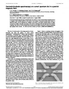
4. Computational domain The computational domain is shown in Figure 1. It extends from Rex = 105 to Rex = 10.6 × 105 . The disturbance strip starts at Rex = 1.6 × 105 and it extends for ∆Rex = 0.15 × 105 . The sponge in the streamwise direction starts at Rex = 9.1 × 105 and extends to the end of the computational domain. The sponge at the inflow extends up to Rex = 1.5 × 105 . The sponge in the wall-normal direction has a thickness of L = δ99 , where δ99 is the boundary layer thickness at Rex = 9 × 105 . The grids used for performing H-type transition are shown in Table 1 along with their resolutions. Unless specified otherwise, all simulations are carried out using grid 1. Grid 1 and grid 2 use one- and eight-million grid points, respectively. The wall units are calculated based on the skin friction from the empirical correlation (White 2006) at Rex = 6 × 105 . This Rex coincides with the location where the overshoot in the skin friction profile in the DNS of Sayadi et al. (2011) appears. The grid resolution study performed by Sayadi & Moin (2010) shows that grid 2 is the coarsest grid producing satisfactory results of the skin friction profile, for both the overshoot and fully developed turbulence regimes in the H-type transition. However turbulent eddy viscosity is negligible on this grid. Therefore, grid 1 is chosen such that the resulting turbulent eddy viscosity is of the

102

T. Sayadi and P. Moin Sponge in the wall normal direction

Laminar inflow

Transitional region

Turbulent section

Sponge and reshaping section

Disturbance strip

Figure 1. Computational domain

Grid Grid points 1 480x160x16 2 960x160x64

∆x+ 90.92 45.46

∆y + 0.93 0.93

∆z + Lx /δ99 Ly /δ99 Lz /δ99 42.99 82.75 4.3 1.3 10.75 82.75 4.3 1.3

Table 1. Characteristics of the different grids for simulations of H-type transition. δ99 is the boundary layer thickness calculated at Rex = 9 × 105 .

same order of magnitude as the molecular viscosity of the flow allowing the assessment of the SGS models.

5. Results The constant coefficient Smagorinsky (CCS) model fails to differentiate between laminar and turbulent flow causing the turbulent eddy viscosity to be active in the laminar section. Because the turbulent eddy viscosity is the same order of magnitude as the molecular viscosity of the flow, the resulting Reynolds number has to be modified by the effective viscosity, νef f = ν + νt , in order to allow the correct comparison between skin friction profiles. The turbulent eddy viscosity in the case of constant coefficient Vreman (CCV) model is an order of magnitude smaller than the molecular viscosity. Therefore, its effect on the Reynolds number is negligible. Figure 2 shows the skin friction profiles of CCS and CCV models versus the modified Reynolds number. The resulting skin friction plots are compared to the DNS of Sayadi et al. (2011) and the laminar correlation. In the case of the CCS, owing to the high turbulent eddy viscosity in the domain, the disturbances produced at the disturbance strip are dissipated instantaneously downstream. For the case of the CCV, the turbulent eddy viscosity is lower than the CCS case. Therefore, the two-dimensional TS wave grows as predicted by linear stability theory. But, the turbulent eddy viscosity is high enough to dissipate the lower amplitude three-dimensional disturbances. Therefore, the nonlinear interactions leading to transition do not take place and the two-dimensional TS wave starts to decay. Both models fail to predict the point of transition. Figure 3 shows the skin friction coefficient for the four dynamic models on grid 1 compared with the DNS of Sayadi et al. (2011). The points of transition where the skin friction diverges from the laminar solution is predicted well by all four models. However, the magnitude of the overshoot in the skin friction is under-predicted by all the models and skin friction in the turbulent regime is much less than in the DNS.

Predicting natural transition using LES

103

0.006

0.005

V2, V5

0.004

Cf

0.003

0.002

0.001 200000

400000

600000

800000

V1, V3, V4 Rex

Figure 2. Skin friction coefficient versus Rex for H-type transition. − − −, DNS Sayadi et al. (2011); -.- , constant coefficient Smagorinsky; —, constant coefficient Vreman model; diamonds, laminar correlation.

0.006

0.005

V2

0.004

Cf

0.003

0.002

0.001 200000

400000

600000

800000

V1, V3 Rex

Figure 3. Skin friction coefficient versus Rex for H-type transition. − − −, DNS Sayadi et al. (2011); -.-, dynamic scale-similarity model; —, dynamic Smagorinsky; -..-, dynamic one equation kinetic energy model; · · ·, global coefficient Vreman model; diamonds, laminar correlation.

The skin friction coefficients obtained from LES with the dynamic Smagorinsky model applied to the two grids in Table 1 are plotted in Figure 4 and are compared to the DNS of Sayadi et al. (2011). It can be concluded that as the grid is refined the prediction of the skin friction coefficient in both the transitional and fully turbulent regimes improve. Figure 5 shows the time and spanwise averaged turbulent viscosity normalized by the free stream molecular viscosity from Rex = 105 to 9 × 105 . The vertical axis in this figure represents the wall normal coordinate. It can be deduced from Figure 5 that the dynamic models become fully active at Rex ' 5 × 105 . This location corresponds to where the skin friction profile diverges from its laminar value, reinforcing the fact that the turbulent viscosity computed dynamically stays close to zero in the early transition stage allowing the disturbances to accurately grow (see Sayadi & Moin 2010). Dynamic scalesimilarity model has a lower value of turbulent viscosity than the dynamic Smagorinsky and dynamic one equation kinetic energy models. This is expected because a portion of

104

T. Sayadi and P. Moin 0.006 0.005

V2, V4

0.004 Cf

0.003 0.002 0.001 200000

400000

V1, V3 Rex

600000

800000

Figure 4. Skin friction coefficient versus Rex for H-type transition. − − −, DNS Sayadi et al. (2011); —, dynamic Smagorinsky (grid 1); · · ·, dynamic Smagorinsky (grid 2); diamonds, laminar correlation.

the stress is carried by the scale-similarity terms. The global coefficient Vreman model produces turbulent eddy viscosity of an order of magnitude smaller than the other three dynamic SGS models. This is to be expected as the model coefficient Cg (see subsection 2.2), is averaged within the entire computational domain including the laminar regime where its value is close to zero. Figure 6 shows the mean streamwise velocity profile normalized by the free stream velocity versus the wall normal direction normalized by the displacement thickness at Reθ = 1210. Dynamic SGS models on grid 1 and dynamic Smagorinsky on grid 2 are compared with the DNS of Sayadi et al. (2011). Dynamic Smagorinsky on grid 2 has the best agreement with the DNS. All the models over-predict the value of the mean velocity close to the wall (y/δ ∗ < 3). Figure 7(a) compares the resulting streamwise intensity normalized by the wall units at Reθ = 1210 for the four dynamic models on grid 1, the dynamic Smagorinsky on grid 2, and the unfiltered DNS. The fine LES agrees well with the DNS data, but the coarse grid LES calculations have a higher peak in the streamwise turbulent intensity compared with the DNS. Among the four dynamic models the one-equation kinetic energy model has the best agreement with the DNS whereas the dynamic Vreman model has the worst agreement. All models agree well with the DNS at y + > 200. Figure 7(b) compares the total normalized Reynolds stress versus wall normal direction in inner wall units. The fine LES has the best agreement with the DNS profile. All the dynamic models on the coarse grid under-predict the peak value of the Reynolds shear stress. This explains the lower value of the skin friction profile in the turbulent section for all these models (Figure 3). To assess the performance of the SGS models for different transition scenarios, the dynamic Smagorinsky model is applied to the K-type transition of Sayadi et al. (2011). The grid resolutions shown in Table 2 are selected such that they are within the same range as grids 1 and 2 used for the H-type transition. It can be deduced from Figure 8 that the dynamic procedure predicts the point of transition accurately in the K-type transition, which is consistent with the predictions of H-type transition. As in the LES of the H-type transition, the SGS models do not seem to produce sufficient Reynolds shear stress in the fully turbulent regime. The results improve as the grid is refined.

Predicting natural transition using LES

105

(a) dynamic one equation kinetic energy model

(b) dynamic Smagorinsky model

(c) dynamic scale-similarity model

(d) Global coefficient Vreman model Figure 5. Time and spanwise averaged turbulent viscosity normalized by the free stream molecular viscosity, ν∞ = 2 × 10−6 .

6. Conclusions LES of natural H- and K-type transitions are performed using six different SGS models with different grid resolutions. The constant coefficient Smagorinsky and Vreman models fail to capture the transition location as indicated by the deviation of the skin friction coefficient. The turbulent viscosity is active throughout the transitional regime, which damps the disturbances and causes the boundary layer to relaminarize. This study shows

106

T. Sayadi and P. Moin 1

0.8

V4, V3

u/U1

0.6

0.4

0.2

0

0

2

4

⇤ Y, V1 y/

6

Figure 6. Mean streamwise velocity versus y/δ ∗ at Reθ = 1210. circles, DNS Sayadi et al. (2011); -.-, dynamic scale-similarity model; —, dynamic Smagorinsky; -..-, dynamic one equation kinetic energy model; · · ·, global coefficient Vreman model; − − −, dynamic Smagorinsky (grid 2).

4.5 4 1

3.5

0 v 0 /u uE, V2 ⌧

u0 /u⌧

RHO_U, V2

3 2.5 2

0.5

1.5 1 0.5 0

0

100

200

Y,y + V1

300

400

500

(a) Stream wise turbulent intensity

0

0

100

200

+ Y,yV1

300

400

500

(b) Reynolds shear stress

Figure 7. Streamwise turbulent intensity and total Reynolds shear stress at Reθ = 1210. circles, DNS Sayadi et al. (2011); -.-, dynamic scale-similarity model; —, dynamic Smagorinsky; -..-, dynamic one equation kinetic energy model; · · ·, global coefficient Vreman model; −−−, dynamic Smagorinsky (grid 2).

that the dynamic SGS models are capable of predicting the point of transition accurately independently of the transition scenario. This is due to the fact that the turbulent viscosity is automatically inactive in the early transitional stage, which allows the disturbances to grow according to linear and non-linear instability theories. The SGS models on a coarse grid under-predict the overshoot of skin friction profile in the transitional regime and also in the turbulent region.

Predicting natural transition using LES

Grid Grid points 3 480x160x16 4 960x160x64

∆x+ 77.38 38.70

∆y + 0.91 0.91

107

∆z + Lx /δ99 Ly /δ99 Lz /δ99 45.79 73.54 3.4 1.29 11.44 73.54 3.4 1.29

Table 2. Characteristics of the different grids for simulations of K-type transition. δ99 is the boundary layer thickness calculated at Rex = 8 × 105 .

0.006

0.005

V2, V4

0.004

Cf

0.003

0.002

0.001 200000

400000

V3,Re V1x

600000

800000

Figure 8. Skin friction coefficient versus Rex for K-type transition. −.−, DNS Sayadi et al. (2011); —, dynamic Smagorinsky (grid 3); − − −, dynamic Smagorinsky (grid 4); diamonds, laminar correlation.

Acknowledgments Financial support from the Department of Energy under the PSAAP program is gratefully acknowledged.

REFERENCES

Chai, X. & Mahesh, K. 2010 Dynamic k-equation model for large eddy simulation of compressible flows. AIAA pp. 2010–5026. Erlebacher, G., Hussaini, M. Y., Speziale, C. G. & Zang, T. 1992 Toward the large-eddy simulation of compressible turbulent flows. J. Fluid Mech. 238, 155–185. Fasel, H. F., Rist, U. & Konzelmann, U. 1990 Numerical investigation of threedimensional development in boundary-layer transition. AIAA 28 (No. 1), 29–37. Germano, M., Piomelli, U., Moin, P. & Cabot, W. H. 1991 A dynamic subgridscale eddy viscosity model. Phys. Fluids A 3 (7), 1760–1765. Ghosal, S., Lund, T. S., Moin, P. & Akselvoll, K. 1995 A dynamic localization model for large-eddy simulation of turbulent flows. J. Fluid Mech. 286, 229–255. Huai, X., Juslin, R. D. & Piomelli, U. 1997 Large-eddy simulation of transition to turbulence in boundary layers. Theoret Comput. Fluid Dynamics 9, 149–163. Kachanov, Y. S. 1994 Physical mechanism of laminar-boundary-layer transition. Annu. Rev. Fluid Mech. 26, 411–482. Kachanov, Y. S. & Levchenko, V. Y. 1984 The resonant interaction of disturbances at laminar-turbulent transition in a boundary layer. J. Fluid Mech. 138, 209–247.

108

T. Sayadi and P. Moin

Lee, J., Choi, H. & Park, N. 2010 Dynamic global model for large eddy simulation of transient flow. Phys. of Fluids 22, 075106. Moin, P., Squires, K., Cabot, W. & Lee, S. 1991 A dynamic subgrid-scale model for compressible turbulence and scalar transport. Phys. of Fluids A 3 (11), 2746–2757. Nagarajan, S., Ferziger, J. H. & Lele, S. K. 2004 Leading edge effects in bypass transition. Report No. TF-90 Stanford University . Park, N., Lee, S., Lee, J. & Choi, H. 2006 A dynamic subgrid-scale eddy-viscosity model with a global model coefficient. Phys. of Fluids 18, 125109. Sayadi, T., Hamman, C. W. & Moin, P. 2011 Direct numerical simulation of Ktype and H-type transitions to turbulence. Center for Turbulence Research Annual Research Briefs . Sayadi, T. & Moin, P. 2010 A comparative study of subgrid scale models for the prediction of transition in turbulent boundary layers. Center for Turbulence Research Annual Research Briefs pp. 237–247. Smagorinsky, J. 1963 General circulation experiments with the primitive equations. i. the basic experiment. Mon. Weather Rev. 91, 99–164. Spalart, P. R. & Watmuff, J. H. 1993 Experimental and numerical study of a turbulent boundary layer with pressure gradients. J. Fluid Mech. 249, 337–371. Vasilyev, O. V., Lund, T. S. & Moin, P. 1998 A general class of commutative filters for LES in complex geometries. J. Comp. Physics 146, 82–104. Vreman, A. W. 2004 An eddy-viscosity subgrid-scale model for turbulent shear flow: Algebraic theory and applications. Phys. of Fluids 16, 3670–3681. White, F. M. 2006 . In Viscous Fluid Flow . Mcgraw-hill International Edition, Third Edition. Yang, Z., Voke, P. R. & Saville, M. A. 1994 Mechanism and models of boundary layer receptivity deduced from large-eddy simulation of by-pass transition. Direct and large-eddy simulation I, Voke et al. (eds.), Kluwer Academic, Dordrecht pp. 225–236. Yoshizawa, A. 1986 Statistical theory for compressible turbulent shear flows, with the application to subgrid modeling. Phys. of Fluids A 29, 2152–2164. You, D. & Moin, P. 2007a A dynamic global-coefficient subgrid-scale eddy-viscosity model for large-eddy simulation in complex geometries. Phys. of Fluids 19 (6), 065110. You, D. & Moin, P. 2008 A dynamic global-coefficient subgrid-scale model for compressible turbulence in complex geometries. Center for Turbulence Research Annual Research Briefs pp. 189–196.