Using Software and Network Measures and Sampling ... vide customers with tailor-made products. ... can be done, for example, by running a benchmark. How-.
Predicting Quality Attributes of Software Product Lines Using Software and Network Measures and Sampling Sergiy S. Kolesnikov
Sven Apel
Norbert Siegmund
University of Passau
University of Passau
University of Magdeburg
Stefan Sobernig
Christian Kästner
Semah Senkaya
Vienna University of Economics and Business
Carnegie Mellon University
University of Munich
ABSTRACT Software product-line engineering aims at developing families of related products, which share common assets, to provide customers with tailor-made products. Customers are often interested not only in particular functionalities (i.e., features), but also in non-functional quality attributes such as performance, reliability, and footprint. Measuring quality attributes of all products usually does not scale. In this research-in-progress report, we propose a systematic approach aiming at efficient and scalable prediction of quality attributes of products. To this end, we establish predictors for certain categories of quality attributes (e.g., a predictor for high memory consumption) based on software and network measures, and receiver operating characteristic analysis. Afterwards, we use these predictors to guide a sampling process that takes the assets of a product line as input and determines the products that fall into the category denoted by the given predictor (e.g., products with high memory consumption). In other words, we suggest using predictors to make the process of finding “acceptable” products more efficient. We discuss and compare several strategies to incorporate predictors in the sampling process.
Categories and Subject Descriptors D.2.8 [SOFTWARE ENGINEERING]: Metrics—Product metrics; D.2.9 [SOFTWARE ENGINEERING]: Management—Software quality assurance; D.2.13 [SOFTWARE ENGINEERING]: Reusable Software
1.
INTRODUCTION
A software product line is a family of related products that share common assets. Products differ in terms of features [3]. A feature is an end-user-visible characteristic that satisfies stakeholder requirements [4]. By using a software product-line approach, a manufacturer designs and implements a family of software products to provide each customer with a tailor-made product.
Permission to make digital or hard copies of all or part of this work for personal or classroom use is granted without fee provided that copies are not made or distributed for profit or commercial advantage and that copies bear this notice and the full citation on the first page. To copy otherwise, to republish, to post on servers or to redistribute to lists, requires prior specific permission and/or a fee. Copyright 20XX ACM X-XXXXX-XX-X/XX/XX ...$15.00.
Variability, reuse, and automated product generation are important goals of product-line engineering. Another important goal is to provide products of required quality. Properties of software, such as time efficiency and memory consumption, are often called quality attributes and cover important aspects of software quality. Quality attributes can be measured by a software manufacturer to ensure that its software adheres to certain standards or customer requirements. Measuring a certain quality attribute of a single product can be done, for example, by running a benchmark. However, benchmarking every single product of a product line turns out to be impractical. In the worst case, the number of products of a product line grows exponentially with the number of features. That is, the number of products may explode. If we consider a product line with hundreds and thousands of features [1], it becomes obvious that productbased measurement does not scale. Therefore, we need better methods for determining quality attributes of all products. We present a systematic procedure for predicting quality attributes of all products of a product line. The prediction procedure uses only statically available information about a product line. In particular, the procedure uses a feature model and data inferred from source code, and makes predictions about runtime behavior of products without executing them. We use data provided by software and network measures. We do not consider run-time data such as workload, input data, exact execution paths, loop boundaries, and many other runtime and environment parameters. We use static data only, because it is much faster to calculate measures on source code and use them in the prediction process than to collect dynamic data from a potentially exponential number of products. The drawback is, however, we cannot make accurate predictions of quantitative values of quality attributes, but we give qualitative statements about products. For example, our algorithm cannot predict the accurate amount of memory required by products, but it can predict which products have low memory consumption compared to other products of a product line. The central part of the prediction procedure is the smart sampling algorithm inspired by game theory. We feed the statically available information about a product line, encoded in a predictor, into the sampling algorithm. The sampling algorithm uses the predictor to predict those products of a product line that have desired quality properties, for example, products with high performance, low memory
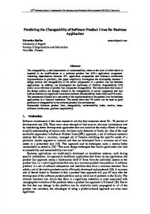
Figure 1: Prediction process overview
consumptions, or small binary footprint. We argue that the sampling that utilizes measure-based predictors, can deliver better results than sampling procedures that treat a product-line as a black-box and do not use any information about the code internals (cf. Section 5). The overall prediction process and the smart sampling as its central part are the main contributions of this researchin-progress report.
2.
PREDICTION PROCESS OVERVIEW
Next, we give a high-level overview of our holistic prediction approach and illustrate it on an example. The prediction process consists of two steps and is outlined in Figure 1. First, we define quality categories for a quality attribute of interest and find predictors for each category. Second, we use these predictors to sample representative feature sets for the quality categories. Based on these feature sets, we predict which products of the product line belong to which quality category. In our example, the quality attribute of interest is the severity of product failures. Our goal is to predict highrisk products (i.e., high-risk feature combinations). That is, products that risk exhibiting high-severity failures if running into error conditions. Step 1: Establishing a Predictor. In this step, we concentrate on the quality attribute of interest, the severity product failures. First, we define two quality categories for this attribute: (1) “High Risk Category” and (2) “Low Risk Category.” At the end of the prediction process, every product of a product line is assigned to one of these categories. Possible failures in the products from “High Risk Category” are likely to be of a relatively high severity. Possible failures in the products from “Low Risk Category” are likely to be of a relatively low severity. To construct a predictor for the “High Risk Category”, we use the NodeRank network measure, which is computed on a static call graph of a system. Bhattacharya et al. found that software components with high NodeRank are more likely to contain high-severity bugs [2]. We do not need an extra predictor for the second category, because products not assigned to the “High Risk Category” by the NodeRank predictor fall into the “Low Risk Category.” A predictor is defined by two ingredients: (1) a measure or a combination of several measures and (2) a corresponding threshold. Let us assume that we have a predictor consisting of a function NR() that computes an aggregated NodeRank for a given set of features, and a threshold T that discriminates between the low and high-risk categories. That is, if we want to categorize a set of features {F1 , F2 }, we apply the function NR() to it and compare the resulting value to the threshold T . If NR({F1 , F2 }) < T , then we assign the feature set to the “Low Risk Category”. If NR({F1 , F2 }) ≥ T , then we assign the feature set to the “High Risk Category”.
We discuss the general problem of finding predictors and their thresholds in Section 3. Using the described categorization procedure, we are able to predict to which category a given feature set belongs. However, how can we make a prediction for all products of a product line? We do not want to calculate NR() for every product, because product-based approach doe’s not scale (cf. Section 1). Our solution is our smart sampling technique, outlined next. Step 2: Sampling. Sampling selects feature sets that we use to judge about quality attributes of the products containing these feature sets. For example, consider a product line with 10 optional and interdependent features (i.e., with 210 products). Features Critical1 and Critical2 are special because all their combinations fall into the “High Risk Category”. That is, for the three possible combinations of these features holds: NR({Critical1 }) ≥ T, NR({Critical2 }) ≥ T, and NR({Critical1 , Critical2 }) ≥ T . Furthermore, products containing one or all three feature sets fall in the “High Risk Category” too. All remaining products fall into the “Low Risk Category.” Using these representative feature sets, we can predict which products fall into which category. Based on this working assumption, reliability predictions for all products of a product line can be made without time consuming analysis of every product. The main task of our smart sampling process is to identify such representative feature sets without measuring every possible feature combination. While this predictive capability of feature sets for entire product populations remains to be validated, there is a strong indication for software systems that the emergent effects (e.g., bottlenecks, failures, etc.) are provoked by a relatively small fraction of the code (i.e., the ”80-20 rule” [9]). Thus, to make predictions about the whole code of a product line, it is sufficient to investigate only this fraction of the code.
3.
ESTABLISHING PREDICTORS
In this section, we describe of a method for establishing predictors for product lines.
3.1
Measurement for Prediction
We leverage information provided by software and network measures that numerically characterize different quality attributes of software. According to the classification given by Fenton et al. [6], we use measures of internal product attributes to predict external product attributes. Product attributes represent different quality aspects of the program code, for example, coupling between source code components or memory consumption of the resulting program. Internal attributes of a product can be measured by analyzing the product on its own. For example, to measure the coupling between two classes of an object-oriented program, we need only the source code of this program. Therefore,
3.2
Finding Good Predictors
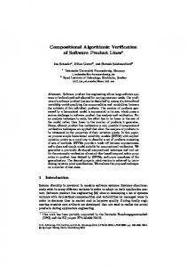
The failure-severity predictor introduced in Section 2 is a binary classifier. Based on a threshold value, it classifies source-code entities into one of two categories. We apply Receiver Operating Characteristic (ROC) analysis to find good thresholds and to evaluate performance of binary classifiers [11]. Next, we illustrate the analysis by an example. The NR() measure of our failure-severity predictor produces values in the range [0, 1]. To find a good threshold for this predictor, we define a set of candidate thresholds (e.g., an interval 0.2-0.6 with a step of 0.1) and establish candidate predictors based on these thresholds. Then, we build a training set of products with known severity of failures that these products have experienced (e.g. using information from a bug database). We use the candidate predictors on the training set to calculate the true positive rate (TPR) and the false positive rate (FPR). If the predictor assigns a product to the “High Risk Category”, we call it a positive result and if it assigns a program to the “Low Risk Category”, we call it a negative result. True positive rate is the relation
True Positive Rate
coupling is an internal product attribute. External attributes of a product can be measured only with respect to its behavior and its environment. For example, to measure the exact memory consumption of a program, we have to know the workload, the platform characteristics, etc. Consequently, memory consumption is an external product attribute. In the example from Section 2 we used a measure of an internal attribute, NodeRank, to predict an external attribute, severity of product failures. In other words, we established a prediction model that relates an internal product attribute to an external products attribute. By supplementing this model with procedures for determining unknown parameters (e.g., thresholds) and procedures for interpreting results (e.g., representative feature sets), we obtain a prediction system [8] that uses internal product attributes to predict external product attributes. Kitchenham et al. showed that a useful prediction system can be created using statistical methods [7]. Following their example, we use a statistical method for discovering relations between internal and external attributes (Section 3.2). We encode information about these relationships in predictors that are purposely bound to a specific product line. Product-line-specific predictors that are established and trained on the source code shared by multiple products can cover relationships between internal and external attributes of the products closer than general predictors. Consequently, product-line-specific predictors can be more useful in predicting external quality attributes of products compared to general predictors. To establish a product-line-specific predictor, we select a small set of products, the training set, from the number of all possible products of a product line. Obviously, we need a criteria for building the training set. For example, we can take a simple random selection of 1% of the products or use domain knowledge to define a training set. We can also use an algorithm that is based on the assumption that products with more structural differences have more differences in their behavior [5]. Thus, including structurally different products into the training set will make the predictor more powerful. We plan to conduct additional experiments to find the best way of constructing the training set.
False Positive Rate A,...,E – candidate thresholds
Figure 2: Example of an ROC Plot
of the number of correct positive results produced by a predictor to the number of test programs actually belonging to the “High Risk Category.” False positive rate is the relation of the number of incorrect positive results produced by a predictor to the number of test programs actually belonging to the “Low Risk Category.” The TPR and FPR values, derived for a given candidate predictor, define one point on an ROC plot (Figure 2). We have defined five candidate predictors based on the five candidate thresholds. After calculating TPR and FPR values for each of these predictors, we have five points (named A to E) on our ROC plot. A predictor having the highest TPR and the lowest FPR has per definition the highest predictive power among all candidate predictors. On an ROC plot, such a predictor is represented by a point that lies nearest to the top-left corner of the plot; in our case, it is predictor C. After finding a predictor with a good threshold, we determine how good the predictor is in classifying products in one of the categories, that is, what its classification performance is. First, we complete the points on the ROC plot to an ROC curve (dashed curve on Figure 2). Subsequently, we compute the area under the ROC curve that measures the classification performance of a predictor and lies in the range [0, 1]. A practical predictor should have a classification performance of 0.7 or higher [11]. By applying ROC analysis to our predictors, we find predictors with good predictive power and we determine if these predictors can be useful.
4.
SMART SAMPLING
Next, we describe our sampling framework and the corresponding smart sampling algorithm.
4.1
Sampling Framework
The main idea of our approach is to incorporate information about the source code of a product line to improve accuracy, scalability, and performance of sampling. Moreover, we aim at building a general feature-sampling framework that is not restricted to certain external quality attributes. There are two preconditions: the availability of good predictors , and the availability of product-line assets, such as source code of features and configuration knowledge (e.g., the feature model). Our sampling framework is supposed to deal with any quality attribute as long as we have good predictors for the quality categories of this attribute. The workflow for the sampling framework is illustrated in Figure 1, Step 2. We provide a predictor for a quality cate-
gory of interest and product line assets (i.e., source code of features and the feature model) to the sampling framework. The sampling algorithm of the framework generates a collection of feature sets. Each of these feature sets belongs to the quality category of interest. Consequently, a product containing one or more of these feature sets will belong to the same quality category, too. Thus, at the end, we can effectively predict which products belong to the quality category of interest that allows us to judge about the corresponding quality attribute of these products.
4.2
Sampling Algorithm
The core of our framework is the sampling algorithm. Its design was inspired by a cooperative game theory. In a cooperative game, agents can build groups and coordinate their actions to achieve better outcomes compared to a situation where they were acting selfishly [10]. Our sampling algorithm models a round-based cooperative sampling game. Features of a product line are agents of the game and their general goal is to build coalitions (i.e., feature sets) with other agents. In each round, an agent can join a coalition of other agents or a coalition can join another coalition to build a larger one. The choice of a coalition to join to is governed by the maximum-value rule. The rule states that the resulting coalition must have the maximum coalition value compared to all possible alternatives. The coalition value is calculated by the predictor supplied to the sampling framework. For example, the value of the coalition {Critical1 , Critical2 } from Section 2 is its NodeRank NR({Critical1 , Critical2 }). At the end of each round, the coalitions with the value above the predictor’s threshold go into the next round. The coalitions with the value below the predictor’s threshold are dismissed. In the next round, the same procedure repeats. The sampling game lasts until no more new coalitions can be built or none of the coalitions can overcome the threshold. At the end of the game, we get representative coalitions (i.e., representative feature sets) that fall into the quality category denoted by the predictor. In the example from Section 2, these resulting coalitions would be the three representative feature sets {Critical1 }, {Critical2 }, and {Critical1 , Critical2 } from the “High-Risk Category.” The predictor strongly influences the process of the sampling game and the quality of the results through its threshold and the calculated coalition values. We can use this important role of the predictor to fine-tune and optimize the sampling-game process. Assume we possess domain knowledge about a certain feature combination. For example, we know that this combination will certainly lead to a higher memory consumption. Then, we tune the predictor such that the value of the coalition containing the feature combination always exceeds the threshold. Thus, we guarantee that this interesting feature combination will be present in one of the resulting coalitions and will help us to predict products with high memory consumption. It is possible that in the first round none of the starting coalitions overcomes the threshold, because their coalition values are too low. Therefore, we start the game with a warm-up phase. During the warm-up phase no coalitions are dismissed even if their values are under the threshold at the end of a round. The warm-up lasts until some coalition exceeds the threshold. This way, we produce at least one feature set of interest at the end of the sampling game.
(a) Base
(b) Symmetric
(c) Asymmetric
Figure 3: Examples of coalition tables
4.3
Sampling Algorithm Variants
We can influence different properties of the sampling algorithm by changing the way coalitions are build. By specifying a rule for building coalitions, we control the following two aspects of the algorithm: (1) how fast the size of coalitions grows and (2) how the number of coalitions changes during the sampling game. These aspects influence the run time of the algorithm and the accuracy of results. We identified three different ways for features to build a coalition and defined corresponding coalition building rules. Based on these rules, we propose three sampling algorithm variants. We use coalition tables to illustrate how these variants work. The differences in constructing these tables in each round of a sampling game reflect different coalition building rules. An example of a coalition table is presented in Figure 3a. For this coalition table, we assume that the corresponding product line has 12 features: A, B,. . . ,F. In the first step, each algorithm variant builds the base table as shown in Figure 3a. The algorithm assigns features of the product line to rows and columns of the base table. One feature for each row and one for each column. This way, each cell of the table represents a feature coalition that consists of the features from the corresponding row and column. A cell contains the coalition value of the corresponding coalition (not shown in the Figure 3a). In the second step, the value of each coalition is calculated. The coalitions with the value above the predictor’s threshold go into the next round. Let’s assume that the coalitions exceeding the threshold are AB, BF, DC and EF (marked red in Figure 3a). We use them in the second round to illustrate different coalition building rules. The remaining coalitions are dismissed. From the second round on, the construction of the coalitions and the coalition table depends on the coalition building rules, which we describe next. Symmetric headers rule. The symmetric headers rule prescribes that the vertical and horizontal headers are symmetric and contain the coalitions coming from the previous round (Figure 3b). This way, the size of coalitions grows fast from round to round: In our example, in the second round, these will be four-feature coalitions, in the third eight-feature coalitions, and so on. The table headers shrink steadily from round to round. Altogether, the number of coalitions reduces with each round, the sampling game evolves rapidly towards termination, and we get the resulting feature sets sooner. On the other hand, smaller coalitions, which may be of interest to us on their own, are not considered and get lost between the rounds. Asymmetric headers rule. This rule gives a chance to smaller coalitions. The horizontal header of the coalition table is the same in every round and always contains single features. The vertical header always contains the coali-
tions coming form the previous round (Figure 3c). This way, we additionally get smaller coalitions (e.g., three-, and fivefeature coalitions), which are not created by the algorithm when it uses the symmetric headers rule. Using the asymmetric headers rule, the sampling game evolves slowly and may take longer to terminate. Due to the constant horizontal header, we have to calculate more coalitions in every round compared to the symmetric header rule. This fact may have negative impact on the algorithm performance. Moreover, the additional smaller coalitions are still forced to grow with each round and will not reach the end of the sampling game. Consequently, the products that could be induced by these smaller coalitions, if they reached the end of the sampling game, are lost. Thus, we consider further game variations that let smaller coalitions survive multiple rounds and potentially reach the end of the sampling game. Diagonal coalitions rule. The symmetric headers rule ignored the coalitions lying on the main diagonal of the table (marked blue in Figure 3b). In contrast, the diagonal coalitions rule allows these to participate in the game. Apart from this, it is analog to the symmetric headers rule. Due to this modification, smaller coalitions can survive multiple rounds and are not forced to grow. Therefore, smaller coalitions that fall into the desired quality category can reach the end of the game. However, the headers do not shrink steadily from round to round. Depending on if and how many diagonal coalitions have survived in the previous round, the headers may shrink or grow. Consequently, the sampling game will evolve faster or slower. Furthermore, the number of coalition-value calculations increases. Consequently, the same performance concerns arise as for asymmetric axes.
5.
RELATED WORK
Measurement for Prediction. Bhattacharya et al. [2] calculated network measures for graph representation of several software projects. The authors successfully used the measurements to make predictions about maintenance effort, bug severity, and defect count for software modules. Eichinger et al. found strong correlations between software measures and runtime behavior [5]. The authors computed software measures, and applied data-mining on them to successfully predict a program’s performance on different hardware architectures. Sampling in Product Lines. Black-box heuristics proved to be effective in predicting external quality attributes of products [12, 13], but they do not take the code into consideration. Our discussed in Sections 3 shows that white-box heuristics that use information extracted from source code can surpass black-box heuristics. Domain knowledge or project-history provide precise information that can be used to judge about quality attributes of products [14, 13]. However, this knowledge is not always available, which reduces general applicability of the technique.
6.
CONCLUSION
Measuring all products of a product line to estimate their quality attributes is not feasible. In this research-in-progress report, we described an ongoing work to efficiently predict quality attributes of all products of a product line. We apply static program analysis to collect information about internal code structure that we use in a sampling process to find
relevant feature sets. Based on these features sets, we predict the quality attribute of interest. Due to the additional information encoded in a predictor, we expect better results compared to other sampling techniques. We implemented the presented sampling algorithm variants, and we prepare a set of predictors to start evaluating the algorithms. We will validate the predictors on a repository of 40 productlines (http://fosd.de/fh) containing C and Java projects of different sizes and from different domains.
7.
REFERENCES
[1] D. Benavides, S. Segura, and A. R. Cort´es. Automated analysis of feature models 20 years later: A literature review. Inf. Syst., 35(6):615–636, 2010. [2] P. Bhattacharya, M. Iliofotou, I. Neamtiu, and M. Faloutsos. Graph-based analysis and prediction for software evolution. In ICSE, pages 419–429, 2012. [3] P. Clements and L. Northrop. Software Product Lines: Practices and Patterns. SEI Series in Software Engineering. Addison-Wesley, 2002. [4] K. Czarnecki and U. Eisenecker. Generative programming - methods, tools, and applications. Addison Wesley, 2000. [5] F. Eichinger, D. Kramer, K. B¨ ohm, and W. Karl. From source code to runtime behaviour: Software metrics help to select the computer architecture. In SGAI, pages 363–376, 2009. [6] N. E. Fenton and S. L. Pfleeger. Software Metrics - A Rigorous and Practical Approach. International Thomson, 1996. [7] B. Kitchenham, L. Pickard, and S. Linkman. An evaluation of some design metrics. Software Engineering Journal, 5:50 –58, 1990. [8] B. Littleword. Forecasting software reliability. In Software Reliability Modelling and Identification, pages 141–206, 1987. [9] P. Louridas, D. Spinellis, and V. Vlachos. Power laws in software. ACM Trans. Softw. Eng. Methodol., 18:2:1–2:26, 2008. [10] N. Nisan, T. Roughgarden, E. Tardos, and V. V. Vazirani. Algorithmic Game Theory. Cambridge University Press, 2007. [11] R. Shatnawi, W. Li, J. Swain, and T. Newman. Finding software metrics threshold values using ROC curves. Journal of Software Maintenance, 22(1):1–16, 2010. [12] N. Siegmund, S. Kolesnikov, C. K¨ astner, S. Apel, D. Batory, M. Rosenm¨ uller, and G. Saake. Predicting performance via automated feature-interaction detection. In ICSE, pages 167–177, 2012. [13] N. Siegmund, M. Rosenm¨ uller, C. K¨ astner, P. Giarrusso, S. Apel, and S. S. Kolesnikov. Scalable prediction of non-functional properties in software product lines. In SPLC, pages 160–169, 2011. [14] J. Sincero, O. Spinczyk, and W. Schr¨ oder-Preikschat. On the configuration of non-functional properties in software product lines. In SPLC, pages 167–173, 2007.