SCIENCE FOR CONSERVATION 323
Predicting the distribution and relative abundance of fishes on shallow subtidal reefs around New Zealand Adam N.H. Smith, Clinton A.J. Duffy and John R. Leathwick
Cover: John Dory (Zeus faber), near Arid Cove Archway, Rakitu Island, Great Barrier Island. Photo: Kim Westerskov. Science for Conservation is a scientific monograph series presenting research funded by New Zealand Department of Conservation (DOC). Manuscripts are internally and externally peer-reviewed; resulting publications are considered part of the formal international scientific literature. This report is available from the departmental website in pdf form. Titles are listed in our catalogue on the website, refer www.doc.govt.nz under Publications, then Science & technical. © Copyright December 2013, New Zealand Department of Conservation ISSN ISBN
1177–9241 (web PDF) 978–0–478–15000–1 (web PDF)
This report was prepared for publication by the Publishing Team; editing by Helen O’Leary and layout by Lynette Clelland. Publication was approved by the Deputy Director-General, Science and Capability Group, Department of Conservation, Wellington, New Zealand. Published by Publishing Team, Department of Conservation, PO Box 10420, The Terrace, Wellington 6143, New Zealand. In the interest of forest conservation, we support paperless electronic publishing.
CONTENTS Abstract
1
1. Introduction
2
2. Methods
3
2.1 Datasets 2.1.1 Diver survey of the abundance of reef fishes 2.1.2 Predictor variables
3 3 3
2.2
Statistical analysis 2.2.1 Fitting BRT models 2.2.2 Grooming models 2.2.3 Weighting of sites 2.2.4 Predictions 2.2.5 Scaling the predictions
7 7 8 8 8 9
2.3
Uncertainty 2.3.1 Bootstrapped confidence intervals 2.3.2 Coverage of the environmental space by samples
3. Results
9 9 10 11
3.1
Model outputs
11
3.2
Influence of the predictor variables
11
3.3
Results for Aplodactylus arctidens 12
3.4
Geographic variation in the reliability of predictions
4. Discussion
15 18
4.1
Predicted patterns of abundance
18
4.2
Measures of uncertainty
18
4.3
Limitations and assumptions
18
4.4
Rare species
19
4.5
Utility and future research
19
5. Acknowledgements
20
6. References
20
Appendix 1 List of reef fish species modelled
23
Appendix 2 Online data files
25
Predicting the distribution and relative abundance of fishes on shallow subtidal reefs around New Zealand
Adam N.H. Smith1,2, Clinton A.J. Duffy3 and John R. Leathwick4,5 1
National Institute of Water & Atmospheric Research Ltd (NIWA), Private Bag 14901, Hataitai, Wellington 6241, New Zealand 2
Present address: Massey University Albany, Private Bag 102904, North Shore 0745, Auckland, New Zealand. Email:
[email protected]. 3
Department of Conservation, Private Bag 68908, Newton, Auckland 1145, New Zealand
4
National Institute of Water & Atmospheric Research Ltd (NIWA), PO Box 11115, Hamilton 3216, New Zealand 5
Present address: Department of Conservation, Private Bag 3072, Hamilton 3204, New Zealand.
Abstract Statistical models of the distribution and abundance of 72 species of rocky reef fishes were developed using boosted regression trees and a set of environmental, geographic and divespecific variables. The models were used to predict and map the occurrence and relative abundance of the selected species on shallow coastal reefs around New Zealand, including the remote Kermadec and Chatham Islands, at the scale of a 1-km2 grid. A cross-validation method indicated that the models were able to explain between 8% (Notoclinops caerulepunctus) and 86% (Chromis dispulis) of the deviance in species abundances, with a mean of 43%. The most widespread species were predicted to be from the family Tripterygiidae, such as Forsterygion flavonigrum, F. malcolmi, and F. varium (predicted at 99%, 99%, and 93% of predicted reef sites, respectively), and also Caesioperca lepidoptera (95%) of Serranidae and Notolabrus fucicola (91%) of Labridae. The models provided here are a valuable source of information for both fish ecologists and managers. The models identify the environmental variables that are ecologically important for these species, and provide insight into the nature of broad-scale relationships between reef fishes and their environment. In particular, a minimum wintertime sea-surface temperature threshold was suggested for many northern species. Moreover, while the biogeography of New Zealand reef fishes has previously been described by reference to regional spatial scales, this is the first known prediction of the distribution of reef fishes for such a broad geographic extent and fine spatial resolution. The predictions from these models thus provide important, spatially-explicit data for use in the management of coastal biodiversity, particularly in the area of marine spatial planning and the identification of high priority areas for conservation. Keywords: biogeography, boosted regression trees, species distribution modelling, rocky reef, reef fish, relative abundance
© Copyright December 2013, Department of Conservation. This paper may be cited as: Smith, A.N.H.; Duffy, C.A.J.; Leathwick, J.R. 2013: Predicting the distribution and relative abundance of fishes on shallow subtidal reefs around New Zealand. Science for Conservation 323. Department of Conservation, Wellington. 25 p. + 2 supplements.
Science for Conservation 323
1
1. Introduction The New Zealand Biodiversity Strategy (DOC & MfE 2000) aims to protect a full range of natural marine habitats and ecosystems in order to effectively conserve New Zealand’s indigenous marine biodiversity. This includes the implementation of a representative network of Marine Protected Areas (MPAs) (DOC & MfE 2000). In order to achieve this aim, central and local government agencies with management responsibility for marine ecosystems, and local communities require detailed information on the spatial distribution of marine resources, and biodiversity values of specific areas and habitat types. Shallow, coastal rocky reefs are focal points for customary, recreational and commercial use, as well as scientific research. It is unsurprising therefore that the majority of marine reserves located around mainland New Zealand are centred upon, or contain, both intertidal and shallow subtidal reef systems (Enderby & Enderby 2006). Fishes form a prominent and taxonomically and ecologically diverse component of these systems (Russell 1983; Paulin & Roberts 1992, 1993; Francis 1996; Clements & Zemke-White 2008). To date, research on distributional patterns of New Zealand reef fishes has been focused at the bioregional scale (Paulin & Roberts 1992, 1993; Francis 1996). Effective marine spatial planning, including development of representative MPA networks, requires information with much finer spatial resolution than this but, as yet, no nationally consistent data sets suitable for this purpose have been published for any New Zealand reef organisms. Unfortunately, it is often prohibitively costly and time-consuming to conduct biological surveys with sufficient fine scale spatial resolution and broad enough geographic coverage for use in systematic marine spatial planning. However, the relationships between species distributions and environmental variables can be determined using statistical models, allowing predictions to be made for areas where observational data are lacking. A variety of modelling techniques are available for this purpose, including an ensemble approach known as Boosted Regression Trees (BRTs, Friedman 2001; Hastie et al. 2001; Elith et al. 2008). Leathwick et al. (2006a) recently used BRTs to model the distributions of demersal fishes at shelf and upper slope depths throughout New Zealand’s Exclusive Economic Zone (EEZ). We used BRTs to model the distribution and relative abundance of rocky reef fishes around the New Zealand coast line using data obtained from diver surveys, and a suite of environmental, geographic and dive-specific predictor variables. The primary objective of this work was to provide fine-scale, nationally consistent data layers that could be used in conjunction with Geographic Information Systems (GIS) and spatial planning tools to inform the management of coastal areas, specifically the identification of priority areas for the conservation and protection of reef fish biodiversity (Leathwick et al. 2008a, b).
2
Smith et al.—Distribution and abundance of fishes
2. Methods 2.1 Datasets
2.1.1
Diver survey of the abundance of reef fishes Data on the relative abundance of reef fishes were obtained from 467 SCUBA dives made around the coast of New Zealand over an 18 year period from November 1986 to December 2004. The majority of the data used in this study were collected by C. Duffy, with a small number collected by A. Smith. The median length of dive was 46 minutes, and the median maximum depth was 17 m. The locations of the sites are shown in Fig. 1. At each site, a thorough search for all species of fish was undertaken. The relative abundance of each species of fish observed was recorded on a scale of 0 to 4 (Table 1). This scale broadly represents orders of magnitude of abundance, and is similar to the so-called ‘Roving Diver Technique’ used by Schmitt & Sullivan (1996), Schmitt et al. (2002) and Semmens et al. (2004). The original dataset contained 212 species. Pelagic, highly cryptic or primarily soft sediment species were excluded from the analysis. With the exception of Anampses elegans, Aplodactylus etheridgii, Epinephelus daemelii, Odax cyanoallix, Trachypoma macracanthus and Zanclistius elevates, species that were too rare to be effectively modelled (i.e. recorded from less than 20 sites) were also excluded from the analysis. Those rare species that were modelled were included at the request of the Department of Conservation (DOC). The final dataset contained 72 species (Table 2; Appendix 1).
2.1.2
Predictor variables Fifteen variables were available to the models, each falling into one of three categories: environmental, geographic and dive-specific (Table 3). Some predictor variables were logtransformed to enable easier visualisation of the results (Table 3). Monotonic transformations have no effect on BRT models or their predictions (Friedman & Meulman 2003).
Environmental predictors Environmental variables were obtained as GIS raster layers. Most were developed as part of the New Zealand Marine Environment Classification (MEC) (Snelder et al. 2004; Snelder et al. 2007). The MEC variable layers of bathymetry, freshwater fraction and orbital velocity were not used because they were considered too inaccurate in shallow (Leathwick, et al. 2004; Snelder et al. 2005; Smith 2006). The latter predicts the velocity of water at the sea bed as induced by swell waves but did not take into account sheltering or refraction by land (Smith 2006). Instead, average fetch, a geographically derived proxy, was used for wave exposure (see below).
Geographic predictors The two geographic variables used were the shortest distance to land and average fetch. The shortest distance to land was calculated using ArcGIS 9.2 and was used as a proxy to represent the complex influence the land has on processes such as sedimentation, primary productivity and larval dispersal. Average fetch is essentially the average distance to land in all directions, and was used here as a surrogate for wave exposure. It was calculated using the method developed by E. Villouta and R. Pickard (described by Fletcher et al. 2005), where the distance to land was measured along 36 radial lines radiating from a point at 10 degrees intervals. Where land was not encountered the lines were cropped at 10 km. Where Fletcher et al. (2005) used the sum of the distances in each direction, we instead used the average distance. This modified index is equivalent, but we consider it more easily interpreted as the average distance to land. This approach to approximating wave exposure has been extended and validated by Burrows et al. (2008).
Science for Conservation 323
3
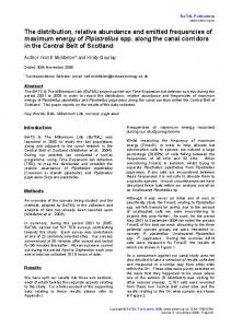
Figure 1. Locations of 467 dive survey sites. The top right and lower right insets show the Kermadec Islands and Marlborough Sounds, respectively. There were no sampling sites at any of the other island groups that are not shown here, including the Chatham Islands.
4
Smith et al.—Distribution and abundance of fishes
Table 1. Ordinal scale of relative abundance of fish recorded at the 467 dive survey sites which comprised the biological data used in this study. This scale broadly corresponds to a y ’ = l n ( y + 1 ) t r a n s f o r m a t i o n o f t h e n u m b e r o f individuals of that species seen per dive. VALUE
NAME
NUMBER OF FISH OBSERVED
0
Absent
0
1
Single
1
Few
2–10
2 3 4
Dive-specific predictors The level of effort and depths of survey dives were not standardised, creating a potential source of bias in the abundance estimates. To control for this, some dive-specific variables were included as predictors in the models and given fixed values for the predictions. These variables were the dive duration, visibility and the minimum and maximum depths surveyed.
The response functions fitted to these variables were forced to be monotonically positive for duration, visibility and maximum Many 11–100 depth, and monotonically negative for minimum depth. The > 100 Abundant assumptions being that poor visibility decreases observed abundance, and that terminating a survey dive some distance below the surface should not increase the observed abundance of a species but may decrease the probability of observing species confined to very shallow water. Allowing these functions to fluctuate freely may allow the model to falsely attribute noise to these dive-specific variables, or falsely attribute variation to them that may be better explained by other variables. Ta b l e 2 . D e t a i l s a n d p e r f o r m a n c e o f t h e b o o s t e d re g re s s i o n t re e m o d e l s f o r e a c h s p e c i e s . T h e n u m b e r o f p re d i c t o r v a r i a b l e s a n d t re e s re l a t e t o t h e c o m p l e x i t y o f t h e m o d e l s . T h e d e v i a n c e e x p l a i n e d i s t h e p ro p o r t i o n o f t h e t o t a l d e v i a n c e i n t h e a b u n d a n c e o f e a c h s p e c i e s t h a t w a s e x p l a i n e d b y t h e m o d e l , a s e v a l u a t e d b y c ro s s - v a l i d a t i o n . T h e p ro p o r t i o n o f t h e p re d i c t i v e re e f s i t e s a t w h i c h t h e s p e c i e s w a s p re d i c t e d ( i . e . n o n - z e ro re l a t i v e a b u n d a n c e ) i s a n i n d e x o f t h e d e g re e t o w h i c h t h e s p e c i e s i s w i d e s p re a d . SPECIES
NUMBER OF PREDICTOR VARIABLES
NUMBER OF TREES FITTED
DEVIANCE EXPLAINED (%)
PROPORTION OF PREDICTIVE SITES OCCUPIED (%)
15
8.2 0.9
Aldrichetta forsteri
8
Amphichaetodon howensis
3
905
58
Anampses elegans
2
9110
78
0.8
Aplodactylus arctidens
8
1825
24
74.1
Aplodactylus etheridgii
2
5165
79
1.4
Atypichthys latus
4
2845
46
1.6
Bodianus unimaculatus
5
2045
77
19.8
Caesioperca lepidoptera
11
6205
46
95.2
Canthigaster callisterna
3
1295
44
0.8
Caprodon longimanus
3
1965
72
6.8
Centroberyx affinis
4
5870
41
9.4
Cheilodactylus spectabilis
8
2310
44
65.5
Chironemus marmoratus
7
990
26
20.7
Chromis dispilus
5
2495
86
21.9
Conger verreauxi
10
1035
8
35.1
Coris sandageri
2
1545
75
6.3
Decapterus koheru
5
1215
39
11.5
820
Epinephelus daemelii
2
4505
69
0.6
Forsterygion flavonigrum
9
2585
43
99.0
Forsterygion lapillum
6
1835
51
45.7
Forsterygion malcolmi
6
2170
39
98.5
12
1440
38
93.2
Forsterygion varium Girella cyanea
2
2705
44
1.2
Girella tricuspidata
6
1080
21
24.7
Grahamina gymnota
8
835
11
19.1 Continued on next page
Science for Conservation 323
5
Table 2 continued
SPECIES
NUMBER OF TREES FITTED
DEVIANCE EXPLAINED (%)
PROPORTION OF PREDICTIVE SITES OCCUPIED (%)
Gymnothorax prasinus
4
945
34
10.9
Helicolenus percoides
8
2640
41
63.6
Hypoplectrodes huntii
9
2330
31
88.2
Hypoplectrodes sp.B
3
1720
67
10.2
10
1090
16
20.0
Kyphosus sydneyanus
6
690
13
12.8
Latridopsis ciliaris
8
1870
38
46.1
Latris lineata
3
1720
47
33.5
10
1160
12
90.0
Mendosoma lineatum
6
2145
30
8.1
Nemadactylus douglasii
5
1550
64
18.6
Nemadactylus macropterus
6
1335
23
55.4
Notoclinops caerulepunctus
8
700
8
72.1
Notoclinops segmentatus
9
1670
30
73.7
Notoclinops yaldwyni
5
1340
40
56.1
Notolabrus celidotus
10
3420
62
72.4
Notolabrus cinctus
5
1390
43
30.7
Notolabrus fucicola
91.1
Karalepis stewarti
Lotella rhacina
11
4215
48
Notolabrus inscriptus
4
2945
38
1.9
Obliquichthys maryannae
7
1755
39
70.0
Odax cyanoallix
3
5360
84
0.2
12
2110
31
72.6
Optivus elongatus
5
1365
31
40.1
Pagrus auratus
5
1605
67
14.5
Parablennius laticlavius
5
1770
60
14.8
Parapercis colias
7
2575
60
84.0
Paratrachichthys trailli
7
1020
14
37.9
Parika scaber
8
3565
41
85.5
Parma alboscapularis
4
1240
62
11.0
Pempheris adspersa
7
2975
63
20.9
Plagiotremus tapeinosoma
2
905
46
4.4
Pseudocaranx dentex
4
745
22
16.8
Pseudolabrus luculentus
2
1245
83
7.2
Pseudolabrus miles
7
2950
50
87.3
Pseudophycis barbata
5
1340
11
52.3
Ruanoho whero
7
1670
32
82.1
Scorpaena cardinalis
2
2260
74
2.7
Scorpaena papillosus
5
1370
36
68.5
Scorpis lineolatus
3
1355
35
53.6
Scorpis violaceus
4
2010
62
15.5
Seriola lalandi
6
990
33
30.0
Suezichthys aylingi
3
1560
47
2.1
Trachurus novaezelandiae
4
840
12
13.9
Trachypoma macracanthus
2
3565
54
0.9
Upeneichthys lineatus
5
2010
45
53.9
Zanclistius elevatus
2
720
13
3.0
Zeus faber
4
675
11
7.5
Odax pullus
6
NUMBER OF PREDICTOR VARIABLES
Smith et al.—Distribution and abundance of fishes
Ta b l e 3 . L i s t o f t h e 1 5 v a r i a b l e s o ff e re d t o t h e m o d e l s , t h e n u m b e r o f m o d e l s i n w h i c h e a c h w a s c h o s e n ( o u t o f n = 72 models, i.e. one for each species) and the average contribution of the variable to the models in which it was used. TYPE
NAME
EXPLANATION
Environmental
sstwint a seabedsal
UNITS
NUMBER OF MODELS IN WHICH THE VARIABLE WAS USED
AVERAGE CONTRIBUTION
Wintertime sea surface temperature
°C
70
33.6
Salinity at the sea bed
psu
43
18.7
sstanampa
Annual amplitude of sea surface temperature
°C
32
18.1
logdisorgma, b
Log of dissolved organic matter
Dimensionless
32
14.9
logtidalspeede
Log of tidal speed
logsuspartmata, b
Log of suspended particulate matter
sstanoma
Sea surface temperature anomaly
logsstgrada
Log of sea surface temperature gradient
chla2a
Concentration of chlorophyll a
Geographic
avefetchc
dcoastd
Dive-specific
a
31
12.0
Approx. g/m3
29
12.2
°C
29
18.8
°C/km
25
11.7
ppm
22
16.2
Average fetch
m
48
12.6
Shortest distance to land
m
7
11.8 12.9
dmax
Maximum depth of dive
dur
Duration of dive
m
17
min
12
dmin
7.6
Mimimum depth of dive
m
10
5.9
vis
Visibility of dive
m
1
5.1
Developed for the MEC (Hadfield et al. 2002; Snelder et al. 2004; Snelder et al. 2007)
b
Pinkerton & Richardson (2005)
c
Produced using a program developed by E. Villouta and R. Pickard (Fletcher et al. 2005)
d
Calculated using ArcGIS
e
Provided by J. Sturman
2.2
Statistical analysis
2.2.1
Fitting BRT models Independent models were used to model the abundance of each of the 72 species of reef fish. All statistical analyses were undertaken in R (R Development Core Team 2007) using a package named ‘gbm’ (Ridgeway 2006) and code developed by Leathwick et al. (2006a, b). The models were built using BRT method. This approach combines many individual regression trees to form a single ensemble model. The regression trees are produced iteratively, gradually improving the overall fit by giving more weight to those sites that are poorly fitted by the previous trees. More complete descriptions of the BRT method can be found in Elith et al. (2008); Friedman (2001); Hastie et al. (2001); Ridgeway (2006). The specifications used in this study were to fit five trees at a time with a learning rate of 0.002 and a tree depth of 5 (see Leathwick et al. 2006a). A Gaussian error distribution was used, as it produced a better overall fit and residual pattern than the alternatives. Because the ordinal scale used in this study to quantify the abundance of fish (Table 1) is roughly logarithmic, this is analogous to using a log-normal approach to modelling abundance, which is common in ecology (Legendre & Legendre 1998). A stepwise, 10-fold, cross-validation procedure was employed to objectively determine the number of trees to be fitted in each model, thus reducing the risk of over-fitting. This approach divides the dataset into 10 subsets, each withheld in turn while models are fitted to each group of 90% of remaining sites. The holdout deviance is then calculated from the average of the prediction errors of the models to the respective withheld subsets. The final number of trees is given by that which minimises the holdout deviance. Goodness-of-fit statistics were calculated
Science for Conservation 323
7
from the cross-validation routine, by taking the mean and standard error of the correlation between the observed and predicted values for the holdout sites. See Hastie et al. (2001) for a more detailed description of the cross-validation method.
2.2.2
Grooming models The models were originally fitted using all available predictor variables. Although the crossvalidation process goes some way to ensure that the models are parsimonious in terms of the number of trees fitted to the data, over-fitting can also occur by including more predictor variables than are necessary. To ameliorate this risk, the global models (those with all predictor variables included) for each species in turn were subjected to a simplification process wherein variables were removed from the models, and then the final models were created by refitting with the reduced variable set. Although the simplification process was essentially subjective, in that it was not done automatically, it was informed by some objective criteria. First, the relative contributions of each variable, in terms of deviance explained, was noted. Second, a procedure was used whereby the lowest contributing variables were sequentially removed from the model, before the model was refitted. The change in deviance explained that resulted from removing a variable was then examined.
2.2.3
Weighting of sites The geographic placement of the dive surveys was neither random nor representative. In fact, their placement was highly skewed, with many more sites occurring in areas where the principal collector (C. Duffy) had done intensive surveys (e.g. the Marlborough Sounds and the Poor Knights Islands). To avoid these areas having a disproportionately high influence on the models, sites were given a weighting that reflected the prevalence of sites with similar environmental characteristics. Sites with environmental characteristics that were poorly represented in the samples were weighted higher, and those with environmental characteristics that were over-represented were down-weighted. To achieve this, a BRT model was used to calculate the probability of a sampling site being present in parts of the environmental space into which predictions are made. For input to this model, the predictive environmental space of interest was represented by 1000 points that were randomly generated from within the predictive domain (produced using Hawth’s Tools for ArcGIS; Beyer 2004). Each of the random points was assigned a value of 0 and each sampling site was assigned a value of 1, and this variable was used to produce a binary response variable that was modelled using the environmental variables. The fitted values were transformed (by the log of the inverse, i.e. log(1/x), where x is the fitted value) and used as the weighting in the predictive models of the abundances of reef fishes. As we were primarily concerned with the environmental representativeness of the sites, only the environmental predictors were used in this model. The majority of the randomly allocated ‘zero’ points were located immediately adjacent to the coast. This was done by selecting them according to a spatially-explicit probability distribution that decreased with distance from the coast. Although, for the final models, predictions were made beyond coastal areas area in the BRT models, the coast is where the most accuracy is required because this is where the majority of sampling sites were located. As a result, the models were more strongly weighted towards, and probably more accurate for, coastal areas.
2.2.4 Predictions A geographic area for which predictions were made (the predictive domain) was delineated. The latitudinal extent of the predictions was from the Kermadec Islands in the north to Stewart Island/Rakiura in the south. Although no surveys were conducted at the Chatham Islands, predictions were made for this remote island group. However, these predictions should be treated with caution as it is known that some mainland species of reef fish have not been recorded there.
8
Smith et al.—Distribution and abundance of fishes
The predictive domain was first produced as a 1-km2 grid, in which a pixel was included if it satisfied at least one of the following conditions: it was within the 50-m depth contour; within 1 km from the shore; or within 1 km of a sample site. This grid was then overlain with a shape file showing the positions of subtidal reefs inferred from navigational charts, and those grid cells that contained no reef were removed. This predictive domain was then converted into a 1-km2 grid of points. Values for the environmental and geographic variables were extracted for each point, and then the BRT models were used to make predictions for each point according to the environmental and geographical conditions. For the dive-specific variables, fixed values were assigned to the predictive points. For duration and visibility, the median values from the surveys were assigned, specifically 46 min and 7 m, respectively. With no reliable bathymetric information available (see section 2.1.2— Environmental predictors), arbitrary depths had to be assigned to the predictive domain. The maximum depth was fixed to 30 m for the entire domain. The minimum depth was fixed to 0 m for points adjacent to the coast (i.e. within 1 km) and 10 m for offshore points. Eight of the predicted species distributions in preliminary modelling showed presences far southwards of their known ranges as given by Francis (2001). These species tended to have a very low number of presences in the dataset. This problem was managed by restricting both the data that were used to produce the model, and the predictions, to northwards of specific latitudes. These species, with their southern latitudinal limits given in parentheses, were Anampses elegans (38°S), Atypichthys latus (38°S), Bodianus unimaculatus (40°S), Girella tricuspidata (40°S), Nemadactylus douglasii (42°S), Notolabrus inscriptus (39°S), Optivus elongatus (43°S) and Trachypoma macracanthus (40°S).
2.2.5
Scaling the predictions Two issues with the raw predictions from the models needed to be overcome. Firstly, because a Gaussian error distribution was used and the fact that predictions from the BRT method are the average taken from many models, the output from these models was on a continuous scale, rather than the ordinal one in the input data. Secondly, the results for many species were poorly scaled, so that the predictions at the lower end of the scale were overestimated and those at the upper end were underestimated. To correct these issues, a second step was used to rescale the predictions to match the original scale of abundance used in the raw data. This involved fitting a single classification tree (using the rpart library in R; see Breiman et al. 1984) to the observed values using the predicted values. The predictions from the entire domain were then rescaled using this model and rounded to one decimal place. Although the rounding to one decimal place meant that the predictions were decimals rather than whole numbers, this method meant that the predicted abundance was unbiased and the original scale of relative abundance was preserved.
2.3 Uncertainty
2.3.1
Bootstrapped confidence intervals Bootstrapped confidence intervals (Manly 1997) were produced to obtain estimates of certainty for each prediction. This was done by refitting the model to each of 500 bootstrap samples of the original data and making predictions (including scaling, see section 2.2.5) for each species. The 0.025 and 0.975 quantiles were taken for every predicted point to provide 95% confidence intervals. These confidence intervals are not presented in this report because of the space required but are available upon request.
Science for Conservation 323
9
2.3.2
Coverage of the environmental space by samples The ‘environmental space’ is the multidimensional space conceived when each environmental variable is treated as a dimension. The samples and predictive sites can be projected into this space according to their values on each environmental variable. Some parts of this environmental space will contain many samples and thus be considered well covered by the biological data. However, because of correlations among the variables (i.e. multicollinearity), other parts of the environmental space will not be well covered by samples. Furthermore, there may be areas in the environmental space for which predictions are made, but which are underrepresented by samples. Here, predictions are considered less reliable and should be treated with a higher degree of scepticism than predictive sites in areas that are well covered by samples. We used a novel approach to quantifying the degree to which the environmental conditions of each predictive site was covered by the samples. The approach was similar to that used in the weighting of sites (see section 2.2.3). A sample of 50 000 random values was taken from the environmental space and assigned a value of 0, indicating that these were ‘false’ sample sites. These were combined with the true samples, to which a value of 1 was assigned. A BRT model was then used to model this new variable that contained 0s for false (random) samples and 1s for true samples, using the Bernoulli error distribution. Predictions using this model then yielded estimates of the probability of a site occurring in each part of the environmental space. Fivehundred trees with an interaction depth of two were used, so that only pair-wise combinations of the environmental variables were regarded. Predictions were then made for the predictive domain using this model, generating values between 0 and 1, according to how well each predictive site was represented by the samples. This may be used as a spatially explicit index of the degree of confidence that can be placed at each cell of the predictive domain, given its environmental conditions.
10
Smith et al.—Distribution and abundance of fishes
3. Results
3.1
Model outputs The primary output of these models is a set of spatially explicit maps that quantify the estimated relative abundance of 72 reef fishes inhabiting shallow coastal waters from Stewart Island/Rakiura north. Predictions were initially made for 52 110 gridded locations, but this was reduced to 9605 when locations that did not contain rocky reef were removed (see section 2.2.4). Presentation of the predictions for each of the 72 species in this document was not possible due to restrictions on space. However, national-scale maps are provided for all modelled species in Supplement 1, and the spatial data underlying these are available on the DOC website associated with this publication (see Appendix 2 for details). The predicted abundance of the marblefish (Aplodactylus arctidens) is presented and discussed in section 3.3. This species had an interesting predicted distribution and illustrates how the broader results may be used and interpreted. The stepwise routine fitted between 675 and 9110 trees to the models, and took between 48 seconds and 46 minutes of computation time (median: 1698 trees and 4 min. respectively). For each species, the deviance in abundance that was explained by the model was evaluated using cross-validated data that were systematically withheld from the modelling process. This is a more robust and conservative method of evaluating goodness-of-fit of a model than using the same data with which the model was trained (Hastie et al. 2001). As assessed by this method, the models were able to explain between 8% (Notoclinops caerulepunctus) and 86% (Chromis dispilis) of the deviance in species abundances (Table 2), with a mean of 43%. Six species that were present at fewer than 20 sites were included in this study because they were of particular conservation interest. Surprisingly, the models for four these species were very successful. Models for these four species (Epinephelus daemelii, Aplodactylus etheridgii, Odax cyanoallix and Anampses elegans) explained between 69% and 84% of the deviance in abundance, while the remaining two of the rare species (Trachypoma macracanthus and Zanclistius elevatus) were among the poorest in terms of deviance explained (Table 2). The predicted percentage of (rocky reef) sites where a species occurs (i.e. predicted abundance was greater than zero) can be used as a measure of the prevalence or ‘widespreadness’ of a species (Table 2). By this criterion, the most widespread species were from the families Tripterygiidae (Forsterygion flavonigrum, F. malcolmi, F. varium, Ruanoho whero), Serranidae (Caesioperca lepidoptera and Hypoplectrodes huntii), Labridae (Notolabrus fucicola and Pseudolabrus miles), Monacanthidae (Parika scaber), Moridae (Lotella rhacina), and Pinguipedidae (Parapercis colias), all of which were predicted at greater than 80% of sites. Most of the rarest species were excluded from the analysis, but the least widespread of those that were modelled were O. cyanoallix (endemic to the Three Kings Islands), E. daemelii, Anampses elegans, Canthigaster callisterna, Amphichaetodon howensis and T. macracanthus, all of which were predicted to occur at less than 1% of sites. The distributions of these species are generally restricted to offshore islands in northern New Zealand.
3.2
Influence of the predictor variables A set of partial dependence plots is provided for all modelled species in Supplement 2. These plots show the marginal effect of each predictor variable on the abundance of the species, after accounting for all the other predictor variables in the model (Elith et al. 2008). Although the partial dependence plots contain a great deal of information about the environmental conditions in which each species is found, there are too many species to discuss them in detail here. However, the overall patterns and importance of the variables across all models are discussed below.
Science for Conservation 323
11
The number of variables selected in the 72 species models ranged from 2 to 12, with a median across species of 5 variables (Table 2). The overall importance of each predictor variable can be quantified by the number of species models in which it was chosen and its average contribution to those models (Table 3). The most consistently important variable for predicting the abundance of species was wintertime sea surface temperature (sstwint), which was selected in 70 (of 72) species models. It was dominant in 30 of these models, with an average of 33% contribution in those models in which it was selected (Table 3). One very consistent pattern noted in the partial dependence plots (see Supplement 2) is that the shape of the response to sstwint forms a threshold for many northern species. Below the threshold the response is near zero or negative and above it is positive. These thresholds are likely to represent the minimum temperature requirements for the species. For example, Chromis dispilus appears to prefer temperatures above 14°C (Fig. 2). There were only two species—Forsterygion lapillum and Trachurus novaezelandiae—for which sstwint was not selected. The next most important variables were average fetch and salinity at the seabed (Table 3). The four dive-specific variables were seldom included in the models, mostly due to their poor predictive power. However, maximum depth of dive was the best predictor for Caesioperca lepidoptera and Forsterygion flavonigrum. This is consistent with these species’ preference for deeper reef habitats (Francis 2001).
3.3
Results for Aplodactylus arctidens The results for Aplodactylus arctidens (marblefish) are presented in more detail to serve as an example of how to interpret the results for the 72 species. The deviance explained by the model (a measure of the overall success of the model at explaining variation in abundance) was 24% (Table 2). This is much lower than the mean of 43% across species, which suggests that the abundance of A. arctidens is less related to the predictor variables than most other species modelled here, and thus less confidence can be placed in the predictions for this species.
0.5 0.0 −0.5 −1.0
fitted function
1.0
1.5
The predicted distribution of A. arctidens spans a wide area from Manawatawhi/Three Kings Islands in the north to Stewart Island/Rakiura in the south and the Chatham Islands in the east (Fig. 3). This is consistent with the known range of this species (Francis 2001). The highest abundance predicted on the ordinal scale was 2, corresponding to up to 10 individuals seen per dive. This species is predicted to occur at relatively high abundance on several stretches of
10
12
14
16
18
sstwint (81.2%) Figure 2. A partial dependence plot of the effect of wintertime sea surface temperature on the abundance of Chromis dispilus (two-spot demoiselle). This is shown as an example of a temperature threshold that drove the predictions for many northern species. It appears that C. dispilus is rarely found in water colder than 14°C.
12
Smith et al.—Distribution and abundance of fishes
30°S
Aplodactylus arctidens Marblefish
35°S 30°S
178°W
175°E
35°S
170°E
178°W
Abundance 0 0.6 0.8 1.5 2.0
40°S
40°S
1.8
44°S
44°S
176°W
45°S
45°S
176°W
170°E
175°E
Figure 3. The predicted abundance of Aplodactylus arctidens (marblefish) on rocky reefs around New Zealand. Abundance was measured on an ordinal scale according to how many individuals were seen on a dive, shown on Table 1. The predicted values were rounded to one decimal place and can be interpreted on the original scale. For example, a predicted abundance of 0.6 means that the expected score on the original scale is between 0 (absent) and 1 (one individual), so that on average a single individual is seen roughly 60% of the time. Likewise, a predicted abundance of 1.5 means that one would expect a score of between 1 (one individual) and 2 (2–10 individuals) at that site, each occurring roughly 50% of the time. The top right and lower right inserts show the Kermadec and Chatham Islands, respectively.
Science for Conservation 323
13
coastline, particularly along the west and northeast coasts of the South Island and the southern part of the North Island. North of Taranaki and Hawke Bay, its predicted abundance is more variable, being predicted to occur in very few areas of the Bay of Plenty and Hauraki Gulf, but becoming more abundant in the far north and at the Three Kings Islands.
14
16
18
−2
−1
0.4 0.0 −0.2 0.0
1.0
−5.5 −4.5 −3.5 −2.5 logsstgrad (12.7%)
0.2
0.4
sstanom (14.7%)
−0.2
0.0
0.2
0.4
sstwint (17.1%)
−0.2 −3
logdisorgm (11%)
−1.5
0.4
12
0.0
0.2 0.0 −0.2
Fitted function
0.4
avefetch (18%)
−4
0.2
0.4 10
0.2
8000
0.0
4000
0
5
15
25
dmin (9.5%)
−0.2
0
−0.2
0.0
0.2
0.4 0.2 −0.2
0.0
0.2 0.0 −0.2
Fitted function
0.4
The effect of each predictor variable on the predicted abundance of A. arctidens is shown in Fig. 4. The most important variable in the model for this species was average fetch (avefetch), with a contribution of 18% relative to the other variables (see Elith et al. 2008). As avefetch is an index of exposure, the corresponding graph in Fig. 4 indicates a positive relationship between exposure and the abundance of A. arctidens. This is reflected in Fig. 3, with the species predicted to be absent from most sheltered reefs, such as those in the Marlborough Sounds, Hauraki Gulf and inner Fiordland. Almost as important as avefetch was wintertime sea surface temperature (sstwint), with the plot suggesting a preference for areas of between 10° and 14°C (particularly 12°C). This species showed negative associations with sea surface temperature anomaly (sstanom) and sea surface gradient (logsstgrad), and less-clear relationships with dissolved organic matter (logdisorgm), tidal speed (logtidalspeed) and suspended particulate matter (logsuspartmat). The strongly decreasing function associated with the minimum depth of the dive (dmin) indicates that this species was mostly seen on dives that included reef in less than 10 m of water (i.e. dmin