AbstractâGeographically dispersed deployments of large and complex multitier ... in California) for load balancing and improved latency to the end users.
Link Gradients: Predicting the Impact of Network Latency on Multitier Applications Shuyi Chen† Kaustubh R. Joshi‡ Matti A. Hiltunen‡ † William H. Sanders Richard D. Schlichting‡ † Coordinated
‡ AT&T
Science Laboratory University of Illinois at Urbana-Champaign Urbana, IL, USA
Labs Research 180 Park Ave. Florham Park, NJ, USA
{schen38,whs}@illinois.edu
{kaustubh,hiltunen,rick}@research.att.com
Abstract—Geographically dispersed deployments of large and complex multitier enterprise applications introduce many challenges, including those involved in predicting the impact of network latency on end-to-end transaction response times. Here, a measurement-based approach to quantifying this impact using a new metric called the link gradient is presented. A non-intrusive technique for measuring the link gradient in running systems using delay injection and spectral analysis is presented, along with experimental results on PlanetLab that demonstrate that the link gradient can be used to predict end-to-end responsiveness, even in new and untested application configurations.
I. I NTRODUCTION The emergence of a global network infrastructure, innetwork services such as cloud computing, and software paradigms such as service-oriented architectures (SOAs) has led to applications that are geographically distributed across data centers around the world. While offering many benefits, such distributed applications introduce significant challenges, not the least of which is the management of end-to-end responsiveness in a highly dynamic environment. In fact, even quantifying the effects of changing network characteristics on end-to-end performance is not easy. For a given deployment of a multitier enterprise application, for example, this relationship depends both on application factors such as execution logic, workloads, configuration settings, and transaction types, and on network factors such as latency, bandwidth, and loss rate. Here, we focus on the impact of logical link latency—that is, the network latency from one application component to another, possibly across multiple physical links—on the endto-end performance of application transactions in multitier applications. While this link latency, as noted above, is not the only factor, it is a significant element in many kinds of distributed applications, especially those deployed across wide geographical areas, as enterprise applications or crossenterprise SOAs often are (e.g., [3], [9]). Our specific goal is to be able to predict accurately the impact of changes in logical link latencies on transaction performance, such as might occur when a distributed application is reconfigured (e.g., a component is moved) or when network routes change. To illustrate the difficulty of this task, consider a 3-tier deployment of the RUBiS web service benchmark [8] on
Local Site (UCSD)
Remote Data Site (SUNY)
Internet User workload
Apache Web Server
MySQL DB
Tomcat App Server
Fig. 1.
Sample RUBiS configuration
PlanetLab, as shown in Figure 1. This configuration reflects a simple scenario in which a company might keep its back-end database server at its local site (in this case, New York), but deploy geographically dispersed front-ends (including some in California) for load balancing and improved latency to the end users. Table I shows the impact on transaction end-to-end response time associated with moving the application server from being colocated with the web server (local) to being colocated with the database (remote). As can be seen, even on this simplest of configurations, the impact of this change in link latency is significant, and varies dramatically based on the transaction type. Not surprisingly, predicting the impact is even more difficult for more complicated and realistic multitier enterprise applications that may have, for example, replicated web, application, and authentication servers and databases, as well as load balancers, caches, firewalls, and traffic filters. Transaction PutBidAuth SearchItemsByReg. SellItemForm ViewBidHistory ViewUserInfo
Local (s) 0.03 5.70 0.04 2.31 4.13
Remote (s) 0.17 0.16 0.14 0.19 0.20
Change 466% -97% 250% -92% -95%
TABLE I AVERAGE RESPONSE TIME FOR RUB I S TRANSACTIONS
In this paper, we present a measurement-based approach to quantifying the impact of changes in logical link latency on the per-transaction end-to-end response time for distributed applications, with a special focus on multitier enterprise applications. The approach is based on the link gradient, a new metric that captures that impact. The collection of link gradients for an application, one per link per transaction type, can then be used to predict end-to-end responsiveness, even in new and untested configurations. We demonstrate the accuracy of these predictions experimentally on PlanetLab using RUBiS
2
II. T ECHNICAL A PPROACH We begin by defining the link gradient of a system, and describe how it can be used to predict the effect of link latency changes on a transaction’s response time. Then, we explain how spectral analysis can allow the computation of a link gradient with only small perturbations to the system and derive the required formulae. A. The Link Gradient Consider a multitier application consisting of multiple software components and let {c1 , c2 , · · · , cn } be the set of n logical one-way communication links between them1 with each link ci parameterized by a link latency li . Further, let the system’s performance metric be quantified using its end-to-end ¯ If the system provides a number of mean response time rt. different services (e.g., it is an e-commerce site with multiple transactions, such as browse and buy), then the response time can be either a per-transaction response time, or the system’s overall mean response time. � rt ¯ quantifies how a change in Then, the link gradient ∇ the link latency for each link affects the response time, and � � ¯ ¯ ∂ rt � rt ¯ = ∂ rt , where each , . . . , is defined as a vector ∇ ∂l1 ∂ln ¯ ∂ rt ¯i = element ∇rt ∂li is the link gradient of link ci . Intuitively, the link gradient of a link is a partial derivative that specifies 1 Two-way communications are represented by two independent links, one for each direction.
0.05
0.1
0.04
0.08
Probability
Probability
and the bulletin-board benchmark RUBBoS [17]. In addition to the metric itself, we also describe an innovative technique for measuring the link gradient in a running system based on delay injection and spectral analysis. This approach has the following advantages: • The use of spectral techniques ensures that intrusiveness is kept to a minimum, thereby allowing link gradient measurements to be performed continuously, even on running production systems. • The link gradient for each transaction can be isolated from other transactions and applications even if they use the same hardware resources, making it particularly useful in highly shared virtual machine environments. • It does not require information about system internals, makes no assumptions about system architecture (e.g., synchronous vs. asynchronous communication or caching policies), does not require modification of the target system, and does not need synchronized clocks. • The metric is simple, is compactly expressed, and can easily be used in conjunction with other system metrics. Knowing the link gradients of a given application provides a cornerstone that can be used in a variety of ways to configure and manage the system. For example, it can be used 1) by designers to ascertain server placements that improve availability while ensuring that responsiveness remains within a tolerable threshold, 2) in SOAs to help in a choice between competing services, or 3) by network operators to evaluate the cost versus benefit trade-offs of planned network upgrades.
0.06 0.04
0.02 0.01
0.02 0 0
0.03
200 400 600 Response time (ms)
800
0 0 2 4 6 8 Converted magnitude (ms) at frequency 0.33Hz
(a) Truncated distribution (b) Distribution at freq. 0.33Hz Fig. 2. Response time distributions
the rate at which the system’s response time changes per unit change in the link latency of communication link ci , assuming that the latencies of all other links remain constant. The link gradient can be used to approximate how the response time of the system would be affected by a change in link latencies (e.g., due to reconfiguration of the system). � = {Δl1 , . . . , Δln } represents Specifically, if the vector Δl the amounts by which all of the link latencies change, the new response time of the system can be approximated by its � ≈ rt( � +O(Δl � 2 ). � rt· ¯ �l+ Δl) ¯ �l)+ ∇ ¯ Δl Taylor expansion, i.e., rt( That equation makes two simplifying assumptions. First, it assumes that the response time (as a function of link latency) is differentiable. Second, the equation only captures first-order effects. If a system’s response time has nonlinear dependencies on the link latency, the equation is accurate only as long as the change in latency Δl is small and the higher-order terms can be ignored. For linear relationships, the higher-order terms vanish, making the equation exact. Although there are some exceptions, we show experimentally under realistic conditions and argue in Section IV that many systems have large regions of continuous linear relationships in which the higher-order effects can be ignored. By doing so, one obtains the following Link Gradient Equation that predicts the end-to-end response time rtb in a configuration b based on the response time rta in another configuration a, and the logical link latencies for each link i in the two configurations—i.e., lia and lib . � � rt(l ¯ i) rtb = rta + (lib − lia ) · ∇ (1) i∈Links
B. Link Latency Perturbation Conceptually, link gradients can easily be computed at runtime by active delay injection. A target communication link can be chosen, and a delay Δli can be systematically injected in the packets traversing the link. The end-to-end response ¯ � can then be measured while the delay time of the system rt is being injected and compared with the nominal response ¯ � −rt ¯ ¯ The ratio rt time rt. Δli is then an approximation to the link � rt ¯ i. gradient ∇ However, in practice, the complicating factor is that production systems, especially those running across wide-area networks and/or on shared resources, typically have response time distributions with long tails, high variances, and nonstationary noise patterns due to periodic events such as garbage collection. For example, Figure 2(a) shows a truncated response time distribution for a single transaction of RUBiS (PutBid) running on PlanetLab. The distribution is constructed
3
using 27648 samples, with a mean of 229 ms and a standard deviation of 269 ms, and has a long tail (not shown) reaching up to 12s. Despite the large number of samples, the 95% confidence interval for the mean is ±3.17 ms, implying that to detect a change in the mean within 10% error, the mean would have to be shifted by at-least 63.4 ms (i.e., by 27%). That would have to be done by adding a low-variance constant delay to every transaction, since attempts to manipulate the mean by introducing larger delays to only a few transactions would increase the variance, and thus the required shift as well. Injecting such large delays into a running system for long periods of time is intrusive, and does not lend itself to dynamic on-the-fly techniques. Moreover, it is also not trivial to inject low-variance delays into communication links. To solve that problem of excessive noise, we propose a unique approach based on the observation that most of the noise found in typical environments is not periodic. Moreover, if periodic noise does exist (e.g., garbage collection), it occurs only at a few narrow frequencies. Therefore, by injecting perturbations in the form of periodic waveforms at carefully chosen frequencies and performing spectral analysis to extract the effect on the system’s response time, one can obtain a level of precision that is significantly superior to that offered by a time domain method. To illustrate how frequency domain analysis can significantly reduce the effects of noise, consider Figure 2(b), which shows a distribution of the magnitude of an arbitrarily chosen frequency component (0.33Hz) from the frequency spectrum of the same response time data represented in Figure 2(a). At this frequency, not only is the mean response time much smaller (1.86 ms), but the distribution is much tighter (with no truncated tail), is more symmetric, and has a standard deviation of 1.1 ms. The corresponding 95% confidence interval of ±0.07 ms allows a change of 1.4 ms to be detected with 10% error. We perform such spectral analysis using the Fast Fourier Transform (FFT) to compute the power spectrum of the response time series. The power spectrum shows the energy present in the waveform as a function of frequency. Because of the non-periodicity of the noise, the energy content at each frequency except the 0 frequency is very low. Therefore, if the delay is injected in a periodic manner at any of those frequencies, its magnitude does not have to be very large. We introduce a periodic delay into the link by using a square wave pattern. When the square wave is high, a constant delay is injected into all the messages that traverse the link. When it is low, no delay is injected. Then, we compute the difference between the energy at the frequency component where we inject the delay and that without delay injection. Finally, we derive the link gradient from the difference as presented in the following subsection. C. Spectral Link Gradient Computation We have developed formulae to show how the power spectrums with and without delay injection can be used to compute the link gradient of the link. We consider some arbitrary response time series xi , i = 0 . . . N − 1 of length N measured
Clients
Front-end Server Logs Sniffer
…
Server Sniffer
Delay
Delay
Central Coordinator
Fig. 3.
Monitoring architecture
at uniform intervals of time ΔTs , called the sampling interval. The final equation to compute the link gradient can be written: π ¯ ) |FFTd (fkd ) − FFT0 (fkd )| · sin( 2n � rt(l ¯ i ) = ∂ rt = ∇ (2) ∂l Δl · kd
In equation 2, FFT0 (fkd ) and FFTd (fkd ) are the complexvalue Fourier Transform of the original response time series without delay injection and the response time series with delay kd , kd = 0 · · · N − 1, is the frequency injection. fkd = N ·ΔT s at which we inject the delay, where kd is the number of complete cycles in the series. 2n = N/kd is the total number of sampling points in each square wave cycle. The complete derivation can be found in [11]. An important point to note is that the phase of the square wave does not appear in the final equation 2. Therefore, the square wave injection, which is done locally at each link, does not have to be synchronized with the end-to-end response time measurement, which is done at the entry point of the system. This eliminates the need for synchronized clocks throughout the system, and makes the technique especially attractive for systems deployed in wide-area settings. III. A RCHITECTURE AND I MPLEMENTATION We have implemented a monitoring framework that automatically calculates the link gradients for one or more distributed applications. Shown in Figure 3 in the context of a single application, the framework consists of a central coordinator and a set of sniffer and delay daemons. The sniffer daemon provides the central coordinator a list of all communication links (identified by source and destination IPs and ports) on which at least one message has been exchanged during the reporting interval. The delay daemon implements delay injection on each node in the system, and starts and stops injection based on commands from the coordinator. To do so, it requires redirection of application packets from each node through the daemon’s process. While there are many ways to achieve such redirection, our current implementation has two mechanisms. The first is based on the loadable packet filter kernel module ip_queue in the standard Linux kernel. Packets are intercepted and their headers routed to the delay daemon through the installation of iptables rules. The second mechanism, used for PlanetLab machines, utilizes the tap device and UDP tunnelling. Applications are configured to use a network interface implemented by the tap device. Designated packets intercepted by the tap device are then tunneled through a UDP connection to the delay daemon. Once the packets have been redirected to the delay daemon
4
process, it uses a timer-wheel implementation [21] to delay the packets by a fixed amount. To correct for inaccuracies, the delay daemon measures the amount of delay actually injected into each packet, and reports the mean for use in the link gradient computation. Both implementations can inject delays accurately up to 1 ms. See [11] for detailed benchmarks and a comparison of the two implementations. The central coordinator orchestrates the daemons and executes the link gradient measurement algorithm. It requires a list of the application’s nodes (host, process) and the location of the end-to-end response time data. Currently, the framework supports applications that have web interfaces, and computes link gradients for each transaction specified using a URL. It parses Apache access logs to extract a response time series— i.e., timestamp, response time pairs—for each transaction URL. No additional workload beyond the application’s normal workload is required for measurement purposes, thus ensuring minimal interference with a running system. The process of measuring the link gradients consists of a training phase and a measurement phase. In the training phase, the coordinator invokes the sniffer daemons to compile a list of all communication links in the application. Then, it passively measures, without any delay injection, the response time series for each transaction to determine the frequency and magnitude of the square wave to inject, and a bin size to construct a uniform time-series from the response time data. The bin size is determined by the workload request rate, and chosen to be large enough so that each bin has at-least one data point. The injection frequency is chosen by partitioning the response time series, computing several FFTs, and choosing the frequency whose magnitude in the FFT has the smallest standard deviation (i.e., has the least noise). Finally, the magnitude of the square wave is chosen to be a multiple of this standard deviation based on how much error the user is willing to tolerate. Next, the coordinator initiates the measurement phase in which, for each logical communication link sniffed in the training phase, it instructs the corresponding delay daemon to inject delays into the packets traversing the link using a square wave pattern, and records the resulting response time series for all application transactions. To avoid injecting excessive delay for links with large link gradients, the square wave magnitude used is initially small, and is adaptively increased up to the maximum computed in the training phase until sufficient accuracy is obtained. The process is conducted for one link at a time and until a sufficient number of response time data points are collected for FFT computation. Finally, equation 2 is used to compute the link gradient for each communication link. A detailed explanation of the measurement algorithm and parameter estimation can be found in [11]. IV. E VALUATION In this section, we evaluate the approach and its predictive power in a realistic setting. Predictive power is evaluated in terms of the link gradient’s ability to predict the application’s response time in a configuration different from the one that
Home Page
View Item
PutBid Auth
Fig. 4.
Users/ λ 20/ 11.15 30/ 17.00 40/ 22.05 50/ 27.80 60/ 33.75
Link WS-AS AS-DB WS-AS AS-DB WS-AS AS-DB WS-AS AS-DB WS-AS AS-DB
Put Bid
Store Bid
Client transition diagram
View PutBid Put Store Item Auth Bid Bid 1.92 1.78 2.04 1.05 15.14 0.63 18.03 18.76 1.47 1.46 1.75 0.68 16.99 0.51 19.13 18.90 1.86 1.78 1.89 1.02 16.28 0.83 18.77 18.19 1.70 2.08 1.58 0.82 18.24 0.46 20.40 20.37 1.48 2.05 1.97 0.87 21.74 0.87 23.15 22.80
λlg 11.05 11.00 16.55 16.60 22.05 21.95 27.70 27.40 33.10 32.65
TABLE II L INK G RADIENTS
was used to compute the link gradient. We show that although the relationship between latency and end-to-end response time changes across varying workloads, configurations, communication models, and load-balancing policies, the link gradient captures those effects. A. Experimental Setup We used a deployment of RUBiS on PlanetLab. RUBiS [8] is a well-known eBay-like auction application that has been extensively used as a benchmark in the literature. Although small, it is representative of many multi-transaction, multitier web applications and can be configured using many settings (e.g., load balancing, connection pooling, and replication) that make it hard to predict the effects of changing logical link latency. To minimize the effect of hardware differences, we chose nodes from PlanetLab with identical configurations. Deployment on PlanetLab nodes distributed across the United States ensured that the measurements were made in a moderately shared, high-variance, and challenging wide-area environment. We used the 3-tier Java-servlet version of RUBiS with a front-end Apache server (WS), middle-tier Tomcat application servers (AS), and a back-end MySQL database server (DB). We used the standard RUBiS workload generator with randomly generated TPC-W client think times [20], and instantiated each client with the bidding-oriented workflow shown in Figure 4. ViewItem (VI) returns information about an item, PutBidAuth (PBA) returns a user authentication page, PutBid (PB) performs authentication and returns detailed bidding information, and StoreBid (SB) stores a bid in the database. Of these, PutBidAuth is application-server-centric, while the other transactions are application- and database-server-oriented. B. Link Gradient Computation We used a setup of RUBiS identical to the one shown in Figure 1 with a single server of each type and the default configuration settings. The workload generator and WS were located in San Diego (UCSD), while AS and DB were located in Pittsburgh (CMU). In all experiments, the link gradient
5
Link Std. Dev. AS-WS DB-AS
Delay (ms) 24 6
View Item 210.78 28.10 65.95
Store Bid 160.5 28.01 94.32
PutBid Auth 82.46 53.82 18.9
Put Bid 151.07 39.25 86.62
TABLE III R ESPONSE T IME P ERTURBATION
Another measure of intrusiveness is the increase in response time due to the delays injected during measurement. Those results are shown for a workload of 30 clients in Table III. The first row indicates the standard deviation of each transaction’s response time during normal system operation, while the other rows show both the injected per-message delay and the change in response time during the measurement process. All numbers are in milliseconds. Although the noisy PlanetLab environment requires much higher delays for some links than an exclusive environment would, the impact is still within the system’s normal behavior. In all cases, one can see that the additional delay is (sometimes significantly) less than the system’s normal standard deviation. One reason for the larger delays is the high variance Tun/Tap injection mechanism on PlanetLab. Based on our experience in local experiments, the injection mechanism based on the standard Linux ip_queue facility requires much less delay injection, and thus less perturbation to the running system.
600
experiment prediction
500 400 300 200 100
700 Response time (ms)
Response time (ms)
700
0
600 400 300 200 100 0
UP UMD DU PU MIT CU Application server location
(a) ViewItem experiment prediction
UP UMD DU PU MIT CU Application server location
(b) StoreBid 700 Response time (ms)
200 180 160 140 120 100 80 60 40 20 0
experiment prediction
500
UP UMD DU PU MIT CU Application server location
Response time (ms)
algorithm was set to use 1 data point per bin, 3456 sampling points per experiment, and a delay scale factor of 30. Table II shows the measured link gradients for all the transactions as the workload was varied from 20 to 60 concurrent clients. It also shows the normal throughput of the system for each workload (λ) and the modified throughput during link gradient measurement (λlg ) for each link. Although we measured the link gradients for both directions of each link (e.g., WS-AS and AS-WS), the table shows the mean value, because the results were very similar. However, as we show later, that may not always be the case, and the ability of our approach to measure link gradient in both directions independently is useful in asymmetric setups such as ADSL lines and satellite links. Comparing the link gradients for the AS-DB link, one can clearly see the difference between the small gradient for the web-server-oriented PutBidAuth transaction and the large gradients for the others (database-oriented). The magnitude of the link gradients provides guidance for targeted application optimization, e.g., moving of components with high link gradients closer together or increasing of cache sizes across such links. The table also shows that the link gradient is not a static metric and increases with workload for all links, possibly due to queuing effects. This observation strengthens our claim that a minimally intrusive runtime technique is desirable for link gradient measurement so that the gradients can be recomputed on-the-fly as the system dynamics change. Finally, the throughput measurements show that the system throughput changes by less than 5% in all cases, thus demonstrating the low intrusiveness of the technique.
600
experiment prediction
500 400 300 200 100 0 UP UMD DU PU MIT CU Application server location
(c) PutBidAuth (d) PutBid Fig. 5. Predicting the effects of component placement
C. Predictive Power Figure 5 demonstrates the link gradient’s predictive power. We use the Link Gradient Equation from Section II-A to predict a transaction’s response time in a new configuration based on its current response time and link latencies, the link gradient, and the latencies in the new configuration. The prediction is compared against a measured response time obtained by actual deployment. To estimate one-way link latency, we compute the mean of 1000 TCP round-trip times, and divide it by two. In the first set of experiments, we kept the workload constant at 30 clients and the locations of our WS and DB fixed at UCSD and CMU respectively, but placed the AS on similar hardware in 6 geographically dispersed locations: Univ. of Pittsburgh (UP), Univ. of Maryland (UMD), Duke Univ. (DU), Princeton Univ. (PU), MIT, and Cornell Univ. (CU). Figure 5 shows the predicted and measured response times for each transaction in each different configuration along with 95% confidence intervals. The confidence interval for the predicted response time rtb in a new configuration b takes into account the errors introduced due to both the response time rta in the original configuration a and the latency measurements in both a and using the equation ρ(rtb ) = �b, and is calculated a b a � rt(l ¯ i )2 , where ρ(rta ), ρ(rt ) + li ∈Links (ρ(li ) − ρ(li )) · ∇ ρ(rtb ), ρ(lia ), and ρ(lib ) are the variances in the response time and latency measurements in configurations a and b, respectively. The results show good agreement between the predicted and measured response times across all transactions even across large response time changes (more than 3x in some cases). Since the hardware and workload in each of the locations were similar, the results demonstrate that link latency plays a dominant role in the application’s response time, and that the link gradient is able to accurately capture the effect of link latency changes on the said response time. In the next set of experiments, we placed WS, AS, and DB at UCSD, UMD, and CMU, respectively, and measured the predictive ability of the link gradients (computed in Table II) as the workload was changed from 20 to 50 concurrent clients.
6
200 100
experiment prediction
0 20
30 40 Workload
200 100
experiment prediction
0 20
50
(a) ViewItem
50
(b) StoreBid
200 150 100 50
experiment prediction
0 20
30 40 Workload
200 100
300 200 100 0
0 VI
SB PBA Transaction type
PB
VI
SB PBA Transaction type
PB
400 300 200 100
experiment prediction
0
50
20
30 40 Workload
50
(c) PutBidAuth (d) PutBid Fig. 6. Prediction results under different workloads
Link AS-WS DB-AS
300
experiment(async) prediction(async) experiment(sync) prediction(sync)
400
(a) Connection pooling (b) Replication mode Fig. 7. Communication pattern effects
500 Response time (ms)
Response time (ms)
30 40 Workload
500
no pool pred no pool pool pred w/ pool
400
Response time (ms)
300
300
Response time (ms)
400
Response time (ms)
Response time (ms)
500
400
500
ViewItem StoreBid PutBidAuth PutBid 2.20 0.98 1.69 1.93 2.87 5.08 0.66 5.87
TABLE IV L INK G RADIENTS WITH C ONNECTION P OOLING
The results presented in Figure 6 show that as the workload increases, the link gradient is able to track the changes in response time across all the transactions to within the limits of experimental error. Note that because separate link gradients are computed independently for the various workloads, the predictions do not suffer from any systemic errors due to higher-order effects as a result of increasing workloads. The results show that the link gradient is a useful predictive tool that can be used by system administrators to evaluate alternative component placements under different workloads. D. Communication Pattern Variations So far we have shown that the link gradient works for a conventional request-response type of application. However, real enterprise systems typically have many different types of communication patterns, such as synchronous and asynchronous calls, load balancing, and connection pooling. To be useful for predicting end-to-end response times in new configurations, the link gradients must be able to automatically capture the effects of such variations. Next, we examine the link gradients’ ability to do so. Connection Pooling. Connection pooling is a technique used to optimize networked applications by recycling connections shared among different requests, thus altering the application’s communication patterns. With connection pooling enabled, requests can use existing connections between the AS and DB rather than initialize a new connection every time. When we computed the link gradients for a workload of 60 clients after enabling connection pooling, we obtained the link gradients shown in Table IV. Comparing the gradients with those for the default setup in Table II, we see, as predicted, that while the gradient on the AS-DB link for the web- and applicationserver-centric PutBidAuth transaction remains relatively unchanged, the link gradients for the other transactions are
Sync AS1-AS2 AS2-AS1 Async AS1-AS2 AS2-AS1
ViewItem StoreBid PutBidAuth PutBid 4.18 4.03 0.15 0.11 4.68 5.24 0.12 0.35 ViewItem StoreBid PutBidAuth PutBid 0.14 0.05 0.10 0.11 0.03 0.03 0.02 0.04
TABLE V L INK G RADIENTS FOR R EPLICATION M ODES
substantially reduced. Figure 7(a) shows the predicted vs. measured response time results in a new configuration (with AS moved from CMU to UMD) both with and without connection pooling. As can be seen from the figure, the predictions match the measured response times to within error tolerances. State Replication. Next, we constructed a scenario with two application servers configured to perform passive sessionstate replication for fault tolerance purposes. The server AS1 is designated as the primary and WS forwards all the requests to it. The application server AS2 is designated as the backup and only receives state updates from AS1. Tomcat allows replication to proceed either synchronously, such that requests do not return to the caller until state transfer to the backup is complete, or asynchronously, such that requests can return before state transfer is complete. Since RUBiS does not use session state, we modified the ViewItem and PutBid transactions to exercise this facility, but left the other transactions untouched. Then, we computed link gradients using both synchronous and asynchronous replication modes with WS in UCSD and DB in CMU as before, but with both application servers placed at the same site (Cornell) because of the replication modes’ multicast requirements. Table V shows the computed link gradients for the link between the primary and backup Tomcat servers under both synchrony settings and in both directions. As shown, the link gradient can clearly distinguish between the two replication modes for the modified transactions. Furthermore, as expected, the synchronous mode has much larger link gradients than the asynchronous mode. However, the asymmetry between the forward and reverse link gradients on the primary-backup link in the asynchronous mode is puzzling, as it is the only such asymmetry we discovered in the entire application. We speculate that the reason for the slight dependency of the response time on the AS1-AS2 link is the interference effects, possibly due to locking, between the threads handling the request and the communications thread responsible for sending the session state to the backup replica. Figure 7(b) shows the predicted vs. measured response times when the link latency between the two application servers was
7
Link AS1-WS AS2-WS DB-AS1 DB-AS2
ViewItem StoreBid PutBidAuth PutBid 1.07 0.60 1.03 0.97 1.00 0.55 0.76 0.76 7.17 9.31 0.09 8.58 7.13 8.96 0.25 8.49
350 300 250 200 150 100 50 0
experiment prediction
VI
SB PBA Transaction type
Response time (ms)
Response time (ms)
TABLE VI L INK G RADIENTS WITH L OAD BALANCING
PB
400 350 300 250 200 150 100 50 0
1 2 4 6 optimal
VI
SB PBA Transaction type
PB
(a) Uniform Load balancing (b) Per Transaction Load Balancing Fig. 8. Load Balancing Effects
increased by 20 ms. (We could not move the servers to a different location due to multicast requirements.) As can be seen, the predictions match the experimental results quite well for all the transactions, showing that the link gradient is able to accurately capture the effects of different communication patterns without requiring any prior information about them. Load Balancing. The last communication pattern we consider is uniform load balancing using Apache’s mod jk module across two identical application servers without any state replication. We computed the link gradients for this scenario with WS in UCSD, and with AS1, AS2, and DB at CMU. The results in Table VI show that, compared with the nonreplicated case in Table II, link gradients are roughly halved for all the links, not just the ones between the WS and ASes. The reason is that the link gradient measures the average effect of changes over time rather than measuring on a per-flow basis. Therefore, the reduction in transaction flows on a link due to upstream load-balancing is reflected as a reduction of the link’s impact on the mean response time, thus reducing the link’s gradient. Figure 8(a) shows that the predicted vs. measured response times show excellent agreement for all transactions when one of the ASes is moved from CMU to UMD. E. Per-Transaction Optimization Link gradients can be used to optimize a system for responsiveness at transaction granularity without detailed application knowledge. Although different transaction types have different optimal locations for the AS (i.e., close to the clients vs. close to the database), the WS can route transaction types differently. Therefore, we can obtain an optimized configuration by having both local and remote AS copies, and using the link gradient to choose which transactions are to be routed to each server. Transactions whose WS-AS gradients are higher than their ASDB gradients are routed to the local server (the PutBidAuth transaction), while all other transactions are routed to the remote server. We conducted experiments using such a setup, with the WS and AS1 at UCSD, and the DB and AS2 at CMU. For comparison, we also conducted experiments in which all requests were load-balanced between the two servers without regard to the transaction type, but using various load-balancing ratios (the
best that can be done without application-specific information). Figure 8(b) shows the measured response time when all the configurations were subjected to a 60-user workload. In the figure, a configuration n means that the requests were routed to the local and remote servers with a ratio of 1:n. The results show that no constant load-balancing ratio can achieve the optimal results that are achieved through the per-transaction load-balancing based on link gradients. Particularly, the link gradients revealed that PutBidAuth transactions only use the WS and the AS. Hence, all such transactions could be routed to the local AS, thus resulting in a dramatically smaller response time compared to any other static load balancing ratio. F. Optimization for Multiple Applications Link gradients can also be used to optimize deployments consisting of multiple applications that share components. For example, consider an ACDN-like scenario [18] in which a company has two applications that share a common back-end database. To optimize the response time for static content, it is willing to use third-party cloud computing solutions to host the front-ends close to the clients, but for privacy and security reasons, wants to host the database in its own data centers. The decision on where to place the database can be affected by how each application uses the database (e.g., synchronous, asynchronous, stored procedure calls, caching, connection pooling) and the application workloads relative to each other. Link gradients can be used to determine at which of many possible locations the back-end should be placed so as to maximize the responsiveness across both applications. To demonstrate that scenario, we used RUBiS and the PHP version of RUBBoS [17], a bulletin board benchmark, as the two applications. We deployed the front-ends for RUBiS (WS and AS) at MIT and for RUBBoS (WS only) at USF (U. South Florida), and consider 3 different locations for the backend database. The response time at each of these possible locations was predicted using the link gradients measured on each application running independently, with a workload of 20 clients each. The link latencies associated with the candidate configurations were measured in the field. Figure 9 shows the measured average response time over all transactions and the predicted response time over all transactions for each application, with the database at each of the possible locations. The results show that the Java-servlet-based RUBiS application is much more sensitive to database server placement than the PHP-based RUBBoS application is (because PHP processing in the web server is a bottleneck for RUBBoS). The average predicted response times using the relative application importance as weights, can be used to make a decision on the best location. More importantly, the results also show that link gradient measurements conducted in isolation for each application can be used to predict, with good accuracy, the response times in shared scenarios. The only experimental measurement that did not fall within the confidence interval for the prediction was for RUBiS when the DB was located at U. Conn. Upon investigation, we discovered that the reason was that the PlanetLab node used at U. Conn. was a much slower
400 350 300 250 200 150 100 50 0
experiment prediction
DUKE
RU Location L ti
UCO11
Response tiime (millisec)
Response ttime (millisec)
8 180 160 140 120 100 80 60 40 20 0
experiment prediction
DUKE
RU Location
UCO11
(b) RUBBoS (a) RUBiS Fig. 9. Predicting the effects of database placement for RUBiS and RUBBoS. (RU: Rutgers, NJ and UConn: U. Connecticut)
machine, with a processor speed of 2.0 GHz (compared to the 3.0 GHz machines used in all the other nodes). By predicting per-transaction response times, the gradients also support reconfiguration of the system if user behavior (i.e., the fraction of each transaction type) change. Although the opportunities for optimization in these applications are limited, the results pave the way for link gradients to be used for response time optimization in larger systems together with search algorithms that allow a systematic exploration of the space of a large number of deployment configurations. Testing the predictions with large production systems, especially those running at AT&T, will be part of our future work. G. Discussion Although our results show that link gradient is an important factor when predicting the impact of the network changes on end-to-end application responsiveness, it is not the only one. When other factors, like machine speed, bandwidth, and loss rates, are drastically changed in the new configuration, link gradients alone might not be enough. We believe that the techniques we have proposed to measure the impact of link latency can be readily extended to these other factors as well, and used to define a class of similar metrics, such as CPU and loss rate gradients. We will do so in future work. The accuracy of the link gradient metric in our experiments is also surprising at first glance because at its core, the link gradient is a linear predictor. However, the reason becomes apparent when an approximate interpretation of link gradients in terms of message crossings is examined. To illustrate, let node a call another node b over a link that has a latency of l, and consider how the mean response time of a would change if the link latency increases by Δl under different types of communication scenarios. If a sends a message to b and waits for a reply before continuing, the response time could be expected to increase by Δl, and the link gradient would be ¯ ¯ rt(l) = 1. The link gradient would remain limΔl→0 rt(l+Δl)− Δl the same if a sent m messages to b in a pipelined fashion before waiting for a response. However, if a were to send m messages in series such that it waited for a response from b before sending the next message, the increased latency would affect the response time for each of the m messages, and the link gradient would be m. Conversely, if a did not wait for a reply from b, an increase in link latency would not affect the response time at all, and the link gradient would be 0. Drawing upon these observations, we can loosely interpret the link gradient as the “mean number of message crossings in the critical path of the system response,” which, for many
communication patterns, is a constant function of node behavior, and thus gives rise to a linear relationship between response time and latency. Factors such as timeouts and increased queuing delay due to large changes in link latency in highly congested systems can affect linearity. However, such conditions are usually exceptions rather than the norm in typically well-provisioned enterprise systems. Furthermore, by increasing the magnitude of the square wave delay injected into the links during the measurement phase and looking for changes in the link gradient (compared to the normal delay injection), our approach can easily detect the latency range over which the linearity assumptions hold and the response time predictions are likely to be accurate. If largemagnitude square waves are to be injected into the system, perturbation can be minimized by reducing the duty cycles of the waveforms (i.e., injecting short spikes of delay rather than square waves). We propose several techniques to address nonlinearity in [11]. In spite of those caveats, the results show that link gradient by itself has excellent predictive value even in a highly heterogeneous and dynamic environment such as PlanetLab (compared to which most enterprise environments are far more stable), and thus we believe that the tool is an invaluable one for system and network administrators in its current form. Investigating other gradients and exploring improved signal injection and processing techniques to further reduce intrusiveness will be part of our future work. V. R ELATED W ORK While we are not aware of any work directly comparable to ours, there has been work on measuring and profiling different aspects of distributed applications for debugging, optimization, modeling, and failure diagnosis. For example, [15] evaluates the impacts of communication overhead and network latency on the performance of parallel applications on tightly coupled clusters by running benchmark applications on an experimental platform where the overhead and network latency can be controlled. Critical path analysis for parallel program execution was introduced in [22] and extended to an on-line version in [13]. The critical path is the longest path in the program activity graph (PAG) that represents program activities (computation and communication), their durations, and their precedence relationships during a single execution of the parallel program. While the critical path can be used to guide debugging and performance optimization in parallel programs, it cannot realistically be used to predict the impact of network latency change on the response time of multitier services. Causal paths indicate how end-user requests flow through system components, and have been used to understand and analyze distributed applications’ performance and to identify bottlenecks [16]. A number of techniques for determining causal paths have been proposed [16], [10], [5], [2], [12], [19], [1], each with its own advantages and disadvantages in terms of assumptions on communication patterns, accuracy, and execution cost. Link gradients intrinsically capture behavior
9
that is very different from causal paths. For example, load balancing causes only local changes in a probabilistic causal graph, while it affects the link gradients of all downstream nodes as shown in Section IV. Although the problem would by no means be trivial, it is conceivable that placement of some restrictions on communication patterns would make it possible to use causal paths to compute the “mean number of message crossings in the path of the system response”, and thus approximate link gradient. However, causal paths cannot capture the effects of increased link latency on other parts of the system (e.g., queuing) and thus cannot measure link gradient exactly. In the literature on the determination of causal paths, only Magpie [5] collects enough information about resource usage along paths that detailed response time modeling might be attempted. However, the need for extensive (albeit lightweight) instrumentation precludes Magpie’s use by hosting providers, such as AT&T, that often do not have the required access to the applications they host. Signal-injection-based techniques have been used by others, mostly for determining failure dependencies. The ADD (Active Dependency Discovery) technique determines failure dependencies by active perturbation of system components and observation of their effects [6]. The ADD approach is generic and does not specify the perturbation and effect measurement methods. In [4], the ADD approach is used with fault injection as the perturbation method. The Automatic FailurePath Interference (AFPI) technique combines pre-deployment failure injection with runtime passive monitoring [7]. While our technique could be seen as a special case of ADD, our technique is far less disruptive to the service provided and can thus be used in running production systems. Delay injection for disk and network access events is used in [12] to verify causal dependencies between such events in a componentbased system. Specifically, [12] uses this technique to determine the object read and write policies in a commodity-based commercial storage cluster. However, the technique is strictly off-line and requires full control of the system workload (including message sizes, types, and frequency). Finally, while Fourier analysis has been used by others to detect periodic behavior in network routing updates [14], we are not aware of any other work in software systems research that uses the specific combination of signal injection and Fourier analysis to improve measurement accuracy. VI. C ONCLUSIONS In this paper, we introduced the link gradient, a new metric that can be used to approximate how the application response time changes with changes in logical link latencies. We presented a novel technique for computing link gradients using signal injection and Fast Fourier Transforms, and described an automatic framework for computing the link gradients of a running multitier enterprise application. We also demonstrated the efficiency and accuracy of our technique using distributed deployments of the RUBiS and RUBBoS applications on PlanetLab and showed that link gradients can be used to predict response times for new and untested configurations.
R EFERENCES [1] AGARWALA , S., A LEGRE , F., S CHWAN , K., AND M EHALINGHAM , J. E2EProf: Automated end-to-end performance management for enterprise systems. In Proc. DSN (June 2007), pp. 749–758. [2] AGUILERA , M., M OGUL , J., W EINER , J., R EYNOLDS , P., AND M UTHITACHAROEN , A. Performance debugging for distributed systems of black boxes. In Proc. SOSP (Oct 2003), pp. 74–89. [3] A LBERT M. L AI , J. N. On the performance of wide-area thin-client computing. ACM Transactions on Computer Systems (TOCS) 24, 2 (May 2006), pp. 175–209. [4] BAGCHI , S., K AR , G., AND H ELLERSTEIN , J. Dependency analysis in distributed systems using fault injection: Application to problem determination in an e-commerce environment. In Proc. 12th Int. Workshop on Distributed Systems: Operations & Management (DSOM) (Oct 2001). [5] BARHAM , P., D ONNELLY, A., I SAACS , R., AND M ORTIER , R. Using Magpie for request extraction and workload modelling. In Proc. OSDI (Dec 2004), pp. 259–272. [6] B ROWN , A., K AR , G., AND K ELLER , A. An active approach to characterizing dynamic dependencies for problem determination in a distributed environment. In Proc. 7th IFIP/IEEE Int. Symp. on Integrated Network Management (IM) (May 2001), pp. 377–390. [7] C ANDEA , G., D ELGADO , M., C HEN , M., AND F OX , A. Automatic failure-path inference: A generic introspection technique for internet applications. In Proc. 3rd IEEE Workshop on Internet Applications (WIAPP) (Jun 2003). [8] C ECCHET, E., M ARGUERITE , J., AND Z WAENEPOEL , W. Performance and scalability of EJB applications. In Proc. OOPSLA (2002), pp. 246– 261. [9] C HAFLE , G., C HANDRA , S., K ARNIK , N., M ANN , V., AND NANDA , M. Improving performance of composite web services over wide area networks. In Proc. 2007 IEEE Congress on Services (SERVICES 2007) (July 2007), pp. 292–299. [10] C HEN , M., K ICIMAN , E., F RATKIN , E., F OX , A., AND B REWER , E. Pinpoint: Problem determination in large, dynamic internet services. In Proc. DSN (June 2002), pp. 595–604. [11] C HEN , S., J OSHI , K., H ILTUNEN , M., S ANDERS , W., AND S CHLICHTING , R. Link gradient: Predicting the impact of network latency on multitier application. Tech. Rep. UILU-ENG-08-2214, University of Illinois, Urbana-Champaign, Sept 2008. [12] G UNAWI , H., AGRAWAL , N., A RPACI -D USSEAU , A., A RPACI D USSEAU , R., AND S CHINDLER , J. Deconstructing commodity storage clusters. In Proc. ISCA (June 2005), pp. 60–71. [13] H OLLINGSWORTH , J. Critical path profiling of message passing and shared-memory programs. IEEE Trans. Parallel Distrib. Syst. 9, 10 (1998), pp. 1029–1040. [14] L ABOVITZ , C., M ALAN , R., AND JAHANIAN , F. Internet routing instability. In Proc. SIGCOMM (1997), pp. 115–126. [15] M ARTIN , R., VAHDAT, A., C ULLER , D., AND A NDERSON , T. Effects of communication latency, overhead, and bandwidth in a cluster architecture. In Proc. ISCA (1997), pp. 85–97. [16] M ILLER , B. DPM: A measurement system for distributed programs. IEEE Trans. on Computers 37, 2 (1988), pp. 243–248. [17] O BJECT W EB C ONSORTIUM. RUBBoS: Bulletin board benchmark. http://jmob.objectweb.org/rubbos.html, Feb 2005. [18] R ABINOVICH , M., X IAO , Z., AND AGGARWAL , A. Computing on the edge: A platform for replicating internet applications. In Proc. 8th Int. Workshop on Web Content Caching and Distribution (Sept 2003). [19] R EYNOLDS , P., W IENER , J., M OGUL , J., AGUILERA , M., AND VAH DAT, A. WAP5: black-box performance debugging for wide-area systems. In Proc. WWW Conf. (May 2006), pp. 347–356. [20] T RANSACTION P ROCESSING P ERFORMANCE C OUNCIL. TPC benchmark W (web commerce) specification, v.1.8. www.tpc.org/tpcw/spec/tpcw V1.8.pdf, Feb. 2002. [21] VARGHESE , G., AND L AUCK , A. Hashed and hierarchical timing wheels: efficient data structures for implementing a timer facility. IEEE/ACM Trans. on Networking 5, 6 (1997), pp. 824–834. [22] YANG , C.-Q., AND M ILLER , B. Critical path analysis for the execution of parallel and distributed programs. In Proc. ICDCS (1988), pp. 366– 373.