Information and Telecommunication Technology Center. Department of ..... flow robustness failure probability. GEANT 2. ATT phys. Sprint phys. 0.0. 0.2. 0.4. 0.6. 0.8 .... We call the new metric Compensated Total Graph Diversity. (cTGD) and ...
Predicting Topology Survivability using Path Diversity Justin P. Rohrer, and James P.G. Sterbenz Information and Telecommunication Technology Center Department of Electrical Engineering and Computer Science The University of Kansas Lawrence, KS 66045, USA Email: {rohrej|jpgs}@ittc.ku.edu Abstract—In this paper we extend our path diversity metric to create a composite compensated total graph diversity metric that is representative of a particular topology’s survivability with respect to distributed simultaneous link and node failures. We tune the accuracy of this metric using 17 topologies, including 3 real fiber maps, 10 inferred logical maps, and 2 synthetic topologies having simulated their performance under a range of failure severities, and present the results. The topologies used are from national-scale backbone networks, with a variety of characteristics, which we characterize using standard graphtheoretic metrics. The end result is a compensated total graph diversity metric that accurately predicts the survivability of a given network topology. Index Terms—path diversitiy; resilience; topology; measurement; survivability
I. I NTRODUCTION AND M OTIVATION With global dependence on networks in general, and the Internet in particular increasing on a daily basis, designing resilience into future networks, and improving the resilience of existing networks is more important than ever. Resilience is the ability of the network to provide and maintain an acceptable level of service in the face of various faults and challenges to normal operation [1], and is a superset of many other metrics including survivability and fault tolerance. In this paper we are interested in quantifying the survivability of network topologies so that new or modified topologies may easily be compared quantitatively. To do this we are starting with the existing path diversity metric that has been shown in our previous work to distinguish between similar topologies according to their survivability. The Path Diversification method [2] is a heuristic algorithm designed to select multiple diverse paths between two nodes in a network. It yields several derived metrics reflecting some of the characteristics of the selected paths, as well as the network as a whole. The later aspect of Path Diversification is what we are interested in for the purposes of this paper. The remainder of this paper is organized as follows: Section II presents some background and related work on survivability and graph theory. Section III. Section IV. Section V, and Section VI concludes. II. BACKGROUND AND R ELATED W ORK While the current Internet architecture makes limited provision for survivability in the higher layers of the network 978-963-8111-77-7
stack, it is clearly a key design consideration when engineering network topologies. This section presents some characteristic examples of existing research and its relation to path diversity. A. Network Survivability The study of network survivability is an extension of the study of fault-tolerance, which is the ability of a system to tolerate faults such that service failures do not result. Fault tolerance generally covers random single or at most a few faults, and is thus a subset of survivability [1]. The current level of reliance on the Internet in modern nations led to the understanding that fault-tolerant designs were not sufficient and that diversity in multiple forms is needed to prevent multiple parts of the infrastructure from sharing fate and thereby protect against correlated failures. Survivability is the capability of a system to fulfill its mission, in a timely manner, in the presence of threats such as attacks or large-scale natural disasters. This definition captures the aspect of correlated failures due to an attack by an intelligent adversary [3], [4], as well as failures of large parts of the network infrastructure [5], [6]. Based on this definition, survivability may encompass a broad spectrum of failure scenarios, however the aspect about which we are concerned in this paper is the ability of a topology to remain connected (the acceptable service) [7], [8] while undergoing multiple simultaneous node and link failures (due to external challenges) [9], [10]. B. Graph Theoretic Approach The problem of finding paths through a network has been well studied in the context of graph theory [11] as well as fiber network planning. The existing algorithms are based on different characteristics of these paths such as shortest paths, diverse and disjoint paths [12], and optical restorability [13]. Several algorithms exist to find the shortest path or kshortest paths that include the earliest algorithms by Ford [14], Moore [15], Dijkstra [16], and Floyd [17], along with several modifications that address negative cycles and improve on or in some cases trade time and space complexities [18]. Following the shortest path between a pair of nodes, several algorithms were proposed to find the k-shortest paths, which involve
RNDM 2011
simple techniques such as manipulation of edge weights to highly optimized algorithms [19]. Furthermore, the concept of diverse paths has been investigated to find a pair of diverse paths, k-diverse paths, and kshortest diverse paths. The existing literature covers techniques based on shortest path algorithm with the incremental removal of used edges from graph transformations [20], [21]. Bhadari presents efficient algorithms to compute edge-disjoint and vertex-disjoint paths [18]. However, these algorithms are based on finding completely diverse paths. Bhandari also discusses an algorithm that finds the maximally diverse paths between a pair of nodes using a modified Dijkstra’s algorithm. This section gives a brief overview of the path diversification mechanism that was originally published in [2], [22]. A. Path Diversity Since the primary motivation for implementing the path diversification mechanism is to increase resilience, paths should be chosen such that they will not experience correlated failures. To this end, we define a measure of diversity that quantifies the degree to which alternate paths share the same nodes and links. Note that in the WAN context in which we are concerned with events and connections on a large geographic scale, a node may be thought of as representing an entire PoP, and a link as the physical bundle of fibers buried in a given right-of-way. This distinction between WAN and LAN component identifiers affects only the population of the path database, not the usage of the diversity metric. A path is any complete set of nodes and links that form a loop-free connection between a node-pair. Given a (source s, destination d) tuple, a path P between them is a vector containing all links L and all intermediate nodes N traversed by that path P = L [ N and the length of this path |P | is the combined total number of elements in L and N . To calculate the path diversity we let the shortest path between a given (s, d) pair be P0 . Then, for any other path Pk between the same source and destination, we define the diversity function D(x) with respect to P0 as: |Pk \ P0 | |P0 |
The path diversity has a value of 1 if Pk and P0 are completely disjoint and a value of 0 if Pk and P0 are identical. P0
0
1
2 P2
3
4
5 P1
Fig. 1.
B. Effective Path Diversity Effective path diversity (EPD) is an aggregation of path diversities for a selected set of paths between a given nodepair (s, d). To calculate EPD we use the exponential function EPD = 1 e ksd where ksd is a measure of the added diversity defined as ksd =
k X
Dmin (Pi )
i=1
III. PATH D IVERSITY OVERVIEW
D(Pk ) = 1
will fail. In our approach, D(P2 ) = 23 , which reflects this vulnerability. P1 on the other hand has a diversity of 1, and does not share any common point of failure with P0 .
Shortest path P0 and alternatives P1 and P2
Figure 1 shows the shortest path, P0 , along with the alternate paths P1 and P2 . Given a failure on node 1, both P0 and P2
where Dmin (Pi ) is the minimum diversity of path i when evaluated against all previously selected paths for that pair of nodes. is an experimentally determined constant that scales the impact of ksd based on the utility of this added diversity. A high value of (> 1) indicates lower marginal utility for additional paths, while a low value of indicates a higher marginal utility for additional paths. Using EPD allows us both to bound the diversity measurement on the range [0,1) (an EPD of 1 would indicate an infinite diversity) and also reflect the decreasing marginal utility provided by additional paths in real networks. This property is based on the aggregate diversity of the paths connecting the two nodes. C. Measuring Graph Diversity The total graph diversity (TGD) is simply the average of the EPD values of all node pairs within that graph. This allows us to quantify the diversity that can be achieved for a particular topology, not just for a particular flow. For example a star topology will always have a TGD of 0, while a ring topology will have a TGD of 0.6 given a of 1. This concludes the overview of the previous work on path diversity. Next we will look at the calculation of topology survivability, before going on to present the new metric compensated total graph diversity. IV. T OPOLOGY S URVIVABILITY C OMPARISON In comparing the survivability of various topologies, we are concerned not with the performance of a particular protocol or mechanism in recovering from failures, rather we are considering the survivability inherent in the structure of the topology itself. To do that, we calculate the flow robustness as the probability of link and node failures is increased. In this case we are considering a flow to be in tact as long as a path exists that connects the source and destination, i.e. the source and destination nodes are not partitioned from one another. Questions of reconvergence time and path protection accuracy are all protocol specific and outside the scope of this paper. We compare 17 topologies, 4 of which are synthetic topologies included for completeness. Ten topologies are logical router-level topologies inferred by the Rocketfuel project [23]. The remaining three are physical-layer fiber topologies based on [24]. Figures 2 and 3 show the physical and logicallayer topologies respectively for the Sprint network, as an
Fig. 2.
Sprint fiber map in KU-TopView
Fig. 3.
1.2
1.2
Full mesh Grid Star Ring
0.8 0.6 0.4
1.0
flow robustness
flow robustness
1.0
0.2 0.0 0.00
Sprint layer-3 map in KU-TopView
Full mesh Grid Star Ring
0.8 0.6 0.4 0.2
0.05
0.10
0.15
0.0 0.00
0.20
0.05
failure probability
Link failure robustness (synthetic)
example of the substantial differences between these two categories of maps. The synthetic topologies can be easily recreated based on the data in the tables below, and the data (including adjacency matrices and node geo-locations) for the real topologies is available via KU-TopView, our Web-based topology map viewer [25]. A. Simulation Results To perform the failure simulations we use MATLAB since we are not looking at dynamic or transient behavior and therefore do not need to simulate packet flows but can perform the calculations using graph-theoretic methods. For each of the 17 topologies we use the following process: 1) load topology adjacency matrix 2) calculate 300 failure sets based on current probability a) 100 sets with link-failures only b) 100 sets with node-failures only c) 100 sets with link & node failures 3) calculate fraction of node-pairs connected in each set 4) average across each 100 sets 5) plot 3 data points 6) increment failure-probability until all values range are complete For this paper we use 51 failure probabilities evenly distributed over the range 0–0.5 inclusive, resulting in 15,300
Fig. 5.
0.15
0.20
Node failure robustness (synthetic)
1.0
Full mesh Grid Star Ring
0.8
flow robustness
Fig. 4.
0.10
failure probability
0.6
0.4
0.2
0.0 0.00
0.05
0.10
0.15
0.20
failure probability
Fig. 6.
Node & link failure robustness (synthetic)
simulation runs for each topology, or 260,100 runs total, which took several days to complete using a computing cluster consisting of approximately 1000 Intel Xeon CPU cores. The results of this process are summarized in Figures 4–12. These plots are a collection of the best-possible or reference curves that would appear on a plot comparing routing or path protection schemes. The curve for each plot is distinct due to its topology, and thus from these plots we can quickly
1.2
1.0
Level 3 AboveNet Exodus EBONE Tiscali Sprint Verio VSNL ATT Telstra
0.8 0.6 0.4
0.8
flow robustness
flow robustness
1.0
0.6
0.4
0.2
0.2 0.0 0.00
Level 3 AboveNet Exodus EBONE Tiscali Sprint Verio VSNL ATT Telstra
0.05
0.10
0.15
0.0 0.00
0.20
0.05
failure probability
Fig. 7.
Link failure robustness (logical)
1.0
0.15
0.20
0.6
Node & link failure robustness (logical)
1.2 1.0
flow robustness
flow robustness
Fig. 9.
Level 3 AboveNet Exodus EBONE Tiscali Sprint Verio VSNL ATT Telstra
0.8
0.4
0.2
0.0 0.00
0.10
failure probability
GEANT 2 ATT phys Sprint phys
0.8 0.6 0.4 0.2
0.05
0.10
0.15
0.0 0.00
0.20
failure probability
Fig. 8.
B. Topology Characteristics Survey Table I lists all of the topologies analyzed, along with a set of standard graph-metrics defined as follows: • Node degree: “The number of connections or edges the node has to other nodes.” [26] • Clustering coefficient: “A measure of degree to which nodes in a graph tend to cluster together.” [27]
0.10
0.15
0.20
failure probability
Node failure robustness (logical)
see which ones are more survivable than others. We have separated the plots into three categories: logical, physical, and synthetic, for plotting purposes simply for readability because they became difficult to distinguish with too many curves in each plot. At this point we can also take note of specific topology’s performance, for example the full-mesh does best overall, while the ring is the worst of the synthetic topologies, and the Sprint and AT&T physical topologies do the worst overall. What we take away from these plots is that the relative ordering of the curves remains largely unchanged (the few exceptions are of minimal size) and so it is reasonable to expect that a measure of survivability may be computed based on the topology alone, without being dependent on the expected probability of failure of individual links and nodes.
0.05
Fig. 10.
• • • •
•
Link failure robustness (physical)
Diameter: The maximum shortest-path between any node-pair. Radius: The minimum of the maximum shortest-path for all nodes. Hop-count: The average shortest-path between all nodeparis. Closeness: “The mean geodesic distance (i.e., the shortest path) between a vertex v and all other vertices reachable from it.” [28] Closeness is a measure of centrality and is related to node degree. Betweenness: “Betweenness is the number of shortest paths passing through a node or link and provides a centrality or importantness measure.” [29]
For each metric, the best (w.r.t. survivability) three values are highlighted in bold. A number of these features are linked to network resilience in one way or another, for example topologies with a high average node-degree generally have more protection paths available, while topologies with a high maximum node or link betweenness may have a central pointof-failure which would be targeted by an attacker. Diameter, radius, and hop-count are closely related distance metrics. In our previous work on path diversification (with a much smaller
TABLE I N ETWORK C HARACTERISTICS Network
Nodes
Links
Full-Mesh Manhattan Grid Ring Star AboveNet AT&T AT&T Phys. EBONE Exodus ´ GEANT2 Phys. Level 3 Sprint Sprint Phys. Telstra Tiscali Verio VSNL
20 25 25 25 22 108 361 28 22 34 53 44 263 58 51 122 7
190 40 25 24 80 141 466 66 51 51 456 106 311 60 129 310 7
Avg. Node Degree 19.00 3.20 2.00 1.92 7.27 2.61 2.58 4.71 4.64 3.00 17.20 4.82 2.37 2.07 5.06 5.08 2.00
1.0
TGD k=4 0.9502 0.8964 0.6321 0.000 0.8559 0.5881 0.9014 0.8635 0.8843 0.7623 0.9154 0.8120 0.8821 0.1295 0.7785 0.8104 0.2001
Clustering Coefficient 1 0 0 0 0.6514 0.3274 0.0550 0.3124 0.3307 0.2898 0.7333 0.3963 0.0340 0.2411 0.5068 0.3509 0.4167
Diam.
Radius
Hopcount
Closeness
1 8 12 2 3 6 37 4 4 9 4 5 37 6 5 8 4
1 4 12 1 2 3 19 3 2 5 2 3 19 3 3 4 2
1 3.3333 6.5 1.92 1.7229 3.3790 13.57 2.2804 2.0563 3.4652 1.7721 2.6882 14.78 3.3025 2.4298 3.1026 2.0952
1 0.3067 0.1538 0.5302 0.5947 0.3030 0.0763 0.4507 0.4978 0.3007 0.5845 0.3853 0.0700 0.3095 0.4236 0.3335 0.4982
1.0
GEANT 2 ATT phys Sprint phys
0.6
0.4
0.2
0.0 0.00
Link Between. 1 54 78 24 21 943 1893 42 22 131 84 129 1637 806 96 480 12
GEANT 2 ATT phys Sprint phys
0.8
flow robustness
flow robustness
0.8
Node Between. 0 110 132 552 196 4160 4527 132 132 556 664 602 3609 2136 656 3736 18
0.6
0.4
0.2
0.05
0.10
0.15
0.20
0.0 0.00
failure probability
Fig. 11.
Node failure robustness (physical)
sample-set of topologies available to work with) it became apparent that the TGD metric was able to differentiate similar topologies according to their survivability performance, but looking at the plots and Table I it is clear that this no longer holds true when the network size varies widely. None of the listed graph theory metrics (or any we are aware of) correlate closely to network survivability as simulated in Section IV-A. We address this void in Section V. V. A NALYSIS In this section we further explore the relationships between the metrics listed in Section IV-B and topology survivability. A. Topology Ranking Based on the flow robustness results (Section IV-A) we can rank the topologies based on their survivability in the presence
0.05
0.10
0.15
0.20
failure probability
Fig. 12.
Node & link failure robustness (physical)
of multiple failures1 as shown in Table II. This ranking can easily be done qualitatively by visual inspection of the plots above, with higher curve outranking lower curves. To perform the ranking a bit more rigorously we chose a fixed point on the x-axis (0.2 in this case) and ranked each topology according to its value at that point on the link and node failure plot. Since the curves have minimal crossover, this produces the same ranking as the visual inspection approach. The metrics values from Table I are also shown here as rankings in order to emphasize the correlation (or lack thereof) between each particular metric and the survivability rank. Some metrics are not included in this table, for example the number of nodes and links that are a direct measure of the graph size, and are not a unique property of the topology design, and the radius, 1 This is not to serve as a recommendation of one network over another for business purposes. Due to common business practices the Internet service ´ providers listed (with the exception of GEANT2) do not make their network topology data publicly available. The data sets used are inferred by third parties and are over 10 years old in some cases
TABLE II N ETWORK R ANK Network Full-Mesh Level 3 AboveNet Exodus EBONE Tiscali Sprint Verio Manhattan Grid VSNL ´ GEANT2 Phys. Star AT&T Telstra Ring AT&T Phys. Sprint Phys.
Survivability Rank 1 2 3 4 5 6 7 8 9 10 11 12 13 14 15 16 17
Node Deg. Rank 1 2 3 5 5 4 5 4 6 7 6 8 7 7 7 7 7
TGD Rank 1 2 8 5 7 11 9 10 4 15 12 17 14 16 13 3 6
Clustering Rank 1 2 3 8 10 4 6 7 15 5 11 15 9 12 15 13 14
which is so closely related to the diameter and the hop-count as to be redundant. In contrast, the average node degree relates the number of nodes to the number of links. From Table II we see that most of the metrics correctly rank the top 2 or 3 networks according to their survivability, but beyond that the rank no longer corresponds. Based on previous experience with the path diversity metrics, and the intuition that diversity should be closely correlated with survivability, we investigated further and developed the Compensated Total Graph Diversity metric. B. Compensated Total Graph Diversity In [2] we noted that the diversity metric is independent of path length, meaning that there is no natural penalty assigned to longer paths as opposed to short ones. On the other hand, there is a significant statistical penalty to long paths when simulating probabilistic failures. Intuitively this penalty results from greater exposure in real networks to component failure due to natural faults or intentional attack. Returning to Table I we see that specific topologies receive a much higher TGD-rank than survivability-rank (e.g. AT&T Physical, Sprint Physical) also have much higher diameters than other networks with similar TGDs. Conversely, the star topology, which is given the lowest TGD rank but performs better than 5 other networks, has a much smaller diameter than the networks it outperforms. Further investigation showed that the average hop-count was a more precise indicator of this penalty than the diameter or radius. Based on this we propose a new composite metric that takes into account both TGD and average hopcount. We call the new metric Compensated Total Graph Diversity (cTGD) and define it as follows: cTGD = eTGD
1
⇥h
↵
(1)
where h is the average hop-count and ↵ is a parameter tuned experimentally. We find that ↵ = 1.25 gives the best
Diam. Rank 1 4 3 4 4 5 5 7 7 4 8 2 6 6 9 10 10
Hopcount Rank 1 2 3 5 7 8 9 10 12 6 14 4 13 11 15 16 17
Closeness Rank 1 3 2 6 7 8 9 10 12 5 14 4 13 11 15 16 17
Node Bet. Rank 1 10 5 4 4 9 8 13 3 2 7 6 14 11 4 15 12
Link Bet. Rank 1 9 3 4 6 10 11 13 7 2 12 5 15 14 8 17 16
correlation to our simulation results. The benefit of taking the exponential of the original TGD is that the range is still bounded between 0 and 1, but is no longer inclusive of 0, which allows for the cTGD of a topology with 0 diversity to be positive, as in the case of the Star network. From the hop-count component we desire an inverse relationship (higher hop-counts result in lower cTGDs), and we use the ↵ parameter to tune the aggressiveness of this relationship. To put equation 1 in the context of providing an end-to-end service, it requires greater diversity to provide a given level of flow reliability over a long path than is required to achieve the same level of flow reliability over a short path. In the graph context, a large-diameter graph must provide a higher TGD to achieve the same level of flow-robustness as a smaller-diameter graph with a lower TGD. TABLE III C OMPENSATED TGD Network Full-Mesh Level 3 AboveNet Exodus EBONE Tiscali Sprint Verio Manhattan Grid VSNL ´ GEANT2 Phys. Star AT&T Telstra Ring AT&T Phys. Sprint Phys.
Survivability Rank 1 2 3 4 5 6 7 8 9 10 11 12 13 14 15 16 17
cTGD 0.9514 0.4494 0.4386 0.3617 0.3113 0.2641 0.2407 0.2009 0.2002 0.1783 0.1668 0.1628 0.1446 0.0941 0.0667 0.0348 0.0307
cTGD Rank 1 2 3 4 5 6 7 8 9 10 11 12 13 14 15 16 17
Table III again shows the topologies ranked according to
their simulated survivability results, alongside their cTGD metric value and cTGD rank. We see that both measures provide an identical ranking for all the topologies suggesting that the cTGD metric is an excellent predictor of topology survivability. We note here that we are not claiming that this exact correlation would hold true for every possible set of topologies, only that we expect a close correlation. The reason for this is that the TGD is a heuristic measure, and the survivability rank is based on a Monte Carlo simulation set, both of with introduce a margin of error. We have sought to reduce this error as much as possible through our methodology. That being said, what we are seeing is a strong correlation so that any reordering should only occur when two topologies have very similar cTGD and survivability metric values to begin with. VI. C ONCLUSIONS AND F UTURE W ORK In this paper we extended the applicability of the total graph diversity metric by compensating for topologies that have higher average hopcounts, thus creating the cTGD metric. Our analysis of the properties of 17 real and synthetic topologies shows that cTGD is an excellent predictor of the survivability of these topologies when simultaneous distributed node and link failures occur. Future work includes evaluating cTGD on a large set of generated topologies engineered with specific properties (node degree, rank, etc.) to characterize the effect of those characteristics on survivability, as well as expanding the scope of our survivability simulations to include various types of intelligently targeted challenges. ACKNOWLEDGMENTS The authors would like to thank the members of the ResiliNets group for discussions which led to this work, in particular Abdul Jabbar. This research was supported in part by NSF FIND (Future Internet Design) Program under grant CNS-0626918 (Postmodern Internet Architecture), by NSF grant CNS-1050226 (Multilayer Network Resilience Analysis and Experimentation on GENI), and by the EU FP7 FIRE programme ResumeNet project (grant agreement no. 224619). R EFERENCES [1] J. P. G. Sterbenz and D. Hutchison. (2008, April) Resilinets: Multilevel resilient and survivable networking initiative wiki. http://wiki.ittc.ku.edu/ resilinets. [2] J. P. Rohrer, A. Jabbar, and J. P. G. Sterbenz, “Path diversification: A multipath resilience mechanism,” in Proceedings of the IEEE 7th International Workshop on the Design of Reliable Communication Networks (DRCN), Washington, DC, USA, October 2009, pp. 343–351. [3] R. Ellison, D. Fisher, R. Linger, H. Lipson, T. Longstaff, and N. Mead, “Survivable network systems: An emerging discipline,” Software Engineering Institute, Carnegie Mellon University, Tech. Rep. CMU/SEI-97TR-013, 1997. [4] J. P. G. Sterbenz, R. Krishnan, R. R. Hain, A. W. Jackson, D. Levin, R. Ramanathan, and J. Zao, “Survivable mobile wireless networks: issues, challenges, and research directions,” in WiSE ’02: Proceedings of the 3rd ACM workshop on Wireless security. New York, NY, USA: ACM Press, 2002, pp. 31–40. [5] R. A. Mahmood, “Simulating challenges to communication networks for evaluation of resilience,” Master’s thesis, The University of Kansas, Lawrence, KS, August 2009.
[6] B. Bassiri and S. S. Heydari, “Network survivability in large-scale regional failure scenarios,” in Proceedings of the 2nd Canadian Conference on Computer Science and Software Engineering (C3S2E). New York, NY, USA: ACM, 2009, pp. 83–87. [7] J. P. Sterbenz, E. K. C ¸ etinkaya, M. A. Hameed, A. Jabbar, and J. P. Rohrer, “Modelling and analysis of network resilience (invited paper),” in Proceedings of the Third IEEE International Conference on Communication Systems and Networks (COMSNETS), Bangalore, India, January 2011, pp. 1–10. [8] J. P. Sterbenz, E. K. C ¸ etinkaya, M. A. Hameed, A. Jabbar, Q. Shi, and J. P. Rohrer, “Evaluation of network resilience, survivability, and disruption tolerance: Analysis, topology generation, simulation, and experimentation (invited paper),” Springer Telecommunication Systems, 2011, (accepted March 2011). [9] E. K. C ¸ etinkaya, D. Broyles, A. Dandekar, S. Srinivasan, and J. P. G. Sterbenz, “A comprehensive framework to simulate network attacks and challenges,” in Proceedings of the 2nd IEEE/IFIP International Workshop on Reliable Networks Design and Modeling (RNDM), Moscow, Russia, October 18–20 2010, pp. 538–544. [10] E. K. C ¸ etinkaya, D. Broyles, A. Dandekar, S. Srinivasan, and J. P. Sterbenz, “Modelling communication network challenges for future internet resilience, survivability, and disruption tolerance: A simulationbased approach,” Springer Telecommunication Systems, 2011, (accepted March 2011). [11] A. Sydney, C. Scoglio, M. Youssef, and P. Schumm, “Characterising the robustness of complex networks,” International Journal of Internet Technology and Secured Transactions, vol. 2, no. 3/4, pp. 291–320, December 2010. [12] W. D. Grover, Mesh-based Survivable Transport Networks: Options and Strategies for Optical, MPLS, SONET and ATM Networking. Upper Saddle River, NJ, USA: Prentice Hall PTR, 2003. [13] W. D. Grover and D. Stamatelakis, “Cycle-oriented distributed preconfiguration: Ring-like speed with mesh-like capacity for self-planning network restoration,” in Proceeding of the IEEE International Conference on Communications (ICC’98), vol. 1, June 1998, pp. 537–543. [14] L. Ford, “Network flow theory,” 1956. [15] E. F. Moore, The Shortest Path Through a Maze. Bell Telephone System, 1959. [16] E. W. Dijkstra, “A note on two problems in connection with graphs,” Numerische Mathematik, vol. 1, pp. 269–271, 1959. [17] R. W. Floyd, “Algorithm 97: Shortest path,” ACM Communications, vol. 5, no. 6, p. 345, 1962. [18] R. Bhandari, Survivable Networks: Algorithms for Diverse Routing. Norwell, MA, USA: Kluwer Academic Publishers, 1998. [19] M. MacGregor and W. Grover, “Optimized k-shortest-paths algorithm for facility restoration,” Software: Practice and Experience, vol. 24, no. 9, 1994. [20] J. W. Suurballe, “Disjoint paths in a network,” Networks, vol. 4, no. 2, 1974. [21] J. W. Suurballe and R. E. Tarjan, “A quick method for finding shortest pairs of disjoint paths,” Networks, vol. 14, no. 2, 1984. [22] J. P. Rohrer, R. Naidu, and J. P. G. Sterbenz, “Multipath at the transport layer: An end-to-end resilience mechanism,” in Proceedings of the IEEE/IFIP International Workshop on Reliable Networks Design and Modeling (RNDM), St. Petersburg, Russia, October 2009, pp. 1–7. [23] (2008, September) Rocketfuel: An ISP topology mapping engine. [24] K. Corporation, “North american fiberoptic long-haul routes planned and in place,” 1999. [25] (2011, January) Resilinets topology map viewer. http://www.ittc.ku.edu/ resilinets/maps/. [26] (2011, May) Wikipedia: Degree distribution. http://en.wikipedia.org/ wiki/Degree distribution. [27] (2011, May) Wikipedia: Clustering coefficient. http://en.wikipedia.org/ wiki/Clustering coefficient. [28] (2011, May) Wikipedia: Centrality. http://en.wikipedia.org/wiki/ Centrality. [29] P. Mahadevan, D. Krioukov, M. Fomenkov, X. Dimitropoulos, K. Claffy, and A. Vahdat, “The Internet AS-level topology: Three data sources and one definitive metric,” ACM Comput. Commun. Rev., vol. 36, no. 1, pp. 17–26, Jan. 2006.