A fast electric load forecasting using adaptive neural ... - IEEE Xplore

Paper accepted for presentation at 2003 IEEE Bologna PowerTech Conference, June 23-26, Bologna, Italy

A Fast Electric Load Forecasting Using Adaptive Neural Networks M. L. M. Lopes, A. D. P. Lotufo, Member, IEEE, and C. R. Minussi

Abstract-This work presents a procedure for electric load forecasting based on adaptive multilayer feedforward neural networks trained by the Backpropagation algorithm. The neural network architecture is formulated by two parameters, the scaling and translation of the postsynaptic functions at each node, and the use ofthe gradient-descendent method for the adjustment in an iterative way. Besides, the neural network also uses an adaptive process based on fuzzy logic to adjust the network training rate. This methodology provides an efficient modification of the neural network that results in faster convergence and more precise results, in comparison to the conventional formulation Backpropagation algorithm. The adapting of the training rate is effectuated using the information of the global error and global error variation. After finishing the training, the neural network is capable to forecast the electric load of 24 hours ahead. To illustrate the proposed methodology it is used data from a Brazilian Electric Company. Index Terms-Adaptive Parameters, Backpropagation Algorithm, Electrical Load Forecasting, Fuzzy Logic, Fuzzy Controller, Neural Networks,Postsynaptic Function.

[IO]. The BP algorithm is considered, in specialized literature, a benchmark in precision. However its convergence is quite slow. This work is divided in two steps: 1)a new formulation of two parameters such as, scaling and translation of the postsynaptic functions is introduced at each neuron, which is adapted in an iterative way using the gradient-descent method [8], and 2)the training rate y is adjusted during the convergence process, to reduce the execution time. The y adjustment is effectuated using a fuzzy controller. It is also used a decaying exponential fun’ctionthat establishes a priority in the regulator actuation in the initial training time and avoids instability in the convergence process. This two implementations are optimal mechanisms that reduces the convergence time and improves the precision of the results. 11. NEURAL NETWORK STRUCTURE

The i-tb output element (neuron) ts, [ I l l is a linear combination of the element inputs x, that are connected to the element i by the weight wq:

I. INTRODUCTION

E

xpansion Planning, Load Flow, Economic Operation, Secunty Analysis and Control of Electric Energy Systems are some studies that effectively depend on the previous behavior of load profile [3], i.e., forecasting of future information of a time series based on past values. In technical literature we can find many methods used to load forecasting such as: simple or multiple linear regression, exponential smoothing, state estimation, Kalman filter, ARIMA of Box and Jenkins [l]. All these methods, to be used, need a previous load modeling for further application. To model the load it is necessary to know some information like: cloudy days, wind speed, suddenly temperature variations and effects of non conventional days (holidays, strikes, etc). After modeling the load using these information, the algorithm is initialized to get the results. The use of neural networks is, nowadays, a very efficient method mainly to the special days case. The objective of this work is to develop a methodology to electric load forecasting using an ANN (Artificial Neural Network) [4], [ I I] with the training by BP (Backpropagation)

Each element can have a bias wo fed by an extra constant input xo = + 1. The linear output 6 is finally converted in a nonlinear function as a sigmoid or relay [4], [ll], etc. The relay functions are appropriated for binary systems, while the sigmoid functions can be employed for both continuous and binary systems.

nI. NEURALNETWORKTRAINING

The BP training is initialized by presenting a pattern X to the network that gives an output Y. Following this, it is calculated an error in each output (the difference with the desired value and the output). The next step is to determine the hack propagated error by the network associated to the partial derivative of the quadratic error of each element related to the weights, and finally adjusting the weights of each element. Then a new pattern is presented, and the process must be repeated until the existence of total convergence ( lerrorl < arbitrated tolerance). The initial M. L. M. Lopes is a PhD. student at UNESP Uha Solteira, SP, Brazil (e- weights are usually adopted as random numbers [ l l ] . The BP algorithm consists of adapting the weights such that the mail [email protected]). A. D. P. Lohlfo is with UNESP Uha Solteira, SP, Brazil (e-mail network quadratic error is minimized. The sum of the [email protected]). C. R. Minussi is with UNESP Uha Solteira, SP, Brazil (e-mail instantaneous quadratic error of each neuron of the last layer (network output) is given by: [email protected]).

0-7803-7967-5/03/$17.00 02003 IEEE

z ,=I no

E'=

E,

2

(2)

where:

K ( r + O = f',(r)+2yPZXr

(7)

= d,-y,;

E,

d, y, no

This way, using the gradient descent method, it is obtained the following schema for adapting the weights [5], [6], [lll:

'

= desired output of the i-th element of the last layer; = output of the i-th element of the last layer: = number of neurons of the last layer.

If the i-th element i s in the last layer, then:

a

=

(8)

4 4

If the i-th element i s in other layers, then: A. Weight Adaptive Process

(9)

Considering the i-th network neuron and using the descendent gradient method, the weight adjustments are formulated by [41, [ I l l :

(3)

where: Q(i) = set of the element indices that are in the next layer to the i-th element layer and are interconnected to the i-th element.

B,(r) = - y [ K(r)l; = stability control parameter or training rate; y (r) = quadratic error gradient related to neuron i weights; Vi & vector containing neuron i weights; = [ WO, WI8 WZi . . . w"r] T.

The yparameter used as a stability control of the iterative process is dependent of 1 [6]. The network weights are randomly initialized considering the interval (0,l). By convenience, the parameter y (training rate) is redefined as follows [5]:

V,( r + l )= V,(r) +'or(r) where:

The adopted direction in (3) to minimize the objective function of the quadratic error corresponds to the gradient opposite direction. The y parameter determines the vector length S, (r). Considering that this work deals with load forecasting (the values are always positive), the nonlinear function to he used is the sigmoid function defined by [4], [ l I ] (varying between 0 and +I): y,= 1 I { ( I + exp (-1zPj +p)t (4) where: 1 = constant that determines the slope of the functiony,; p = constant that determines the translation of the function y,. The gradient 0, (r) is represented by:

y = r'1n

(10)

Replacing (10) in (7), it is "cancelled" the amplitude dependency of U related to A. The U amplitude is maintained constant to every I This alternative is important considering that L only actuates in the left and right tails of U. Then, (7) is written as follows[5]:

V,( r + O = V,(r) + 12r' P, I

t X,

The BP algorithm is considered in the technical literature a benchmark in precision, although its convergence is very slow. In this way, this work proposes to adjust the training rate 11 during the convergence process taking as an objective the reduction in the execution training time. The r' adjustment is executed by a proceeding based on a fuzzy controller.

B. Slop Adaptive Process of Sigmoid Function Differentiating (2) in relation to the vector Vi, it is obtained the following equation: ay,_ _ _as =__=

av,

ay, a ~ =, Uz azs,

av, a q a v ,

4

& sigmoid function derivative, (4), related to =

a; (6)

a y , ( I -YJ.

Then,

where: X, pattern vector; = [ xo, X I , XI, . . .

K = f (A pa zp, w.,

av,

where:

The general form of the postsynaptic functions used to adjust the neural network is given by [8]:

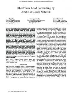
The scaling and translation parameters contain corresponding learning rates denoted by yh, and yp, respectively. A generalized architecture of a neuron with A and p perfomng the role of scaling and translation in a multidimensional space is showed in Fig. 1 [SI:

P Xnr

1 T.

(11)

Fig 1. AIchitecfure of the neural network

The adjustment of the scaling and translation of the postsynaptic functions is developed by the gradient descendent method based on the BP algorithm. Similar to the calculation of adjusting the weights, the adjustment of the inclination and translation parameters of the sigmoid function is effectuated considering the i-th neuron, by the descent gradient method. This way, the adjustment of the inclination parameter of the sigmoid function is given by [8]:

A ( r + O = A ( r )+ 0; ( r )

= [POI PI, Pz, . . . P", IT.

The gradient

Ep is represented by:

Now, differentiating (2) in relation to the vector pi, it is obtained the following equation:

(12)

where:

n

WI; 0; (r) = Ea@)= quadratic error gradient related to neuron i slope; vector containing neuron i slopes; A, = [.lo, 1 1 , & . . . ,LIT.

where: op A sigmoid function deriv;itive, (4), related top,; = Y , (1 -n). The following equation defines the adaptation rule of the translation parameter of the nonlinear function [8]:

The gradient Eais represented by [81:

p , ( r + O = pr(') + 2ypPp; If the i-th element is in the last layer, then: Now, differentiating (2) in relation to the vector obtained the following equation [8]:

A,it is

Pp

=

qx4

(16)

If the i-th element is in other hyers, then:

where:

oh p sigmoid function derivative, (4), related to A;

= fi,Y,(l-Y,). Then, the rule that defines the adaptation of the inclination parameter of the sigmoid function is given by the following equation:

A.(r+I)=&(r)+2nPh If the i-th element is in the last layer, then:

PA, = oh 4

IV. NEURALNETWORKW rnFUZZY CONTROLLER (13)

If the i-th element is in other layers, then:

BAi = oh

c

wvP4

The adaptation rule for inclination and translation parameters of the network is calculated in an iterative way for every i-th neuron. Therefore, the adaptive neural network always gives an output, and the network is faster than the conventional one. The next step is to introduce the fuzzy controller, which objective is to execute a control on the training rate to obtain a better solution.

(14)

i E Q(i)

C. Shift Adapfive Process of Sigmoid Funcfion Using the same schema, the sigmoid function translation Darameter is formulated by:

The purpose of the fuzzy controller is to reduce the execution training time through the adjustment of the training rate p.The basic idea of the methodology consists of determining the system state, defined as the global error %and the global error variation A%, @.kingas ai objective a control structure Ayl that leads the error to zero in a reduced iteration number, when compared to the conventional procedures. In this work, the control is formulated using the fuzzy logic is defined as: concepts ,91. Initially, the

where: np = number of the network pattern vectors. E p ( r )= quadratic error gradient related to neuron i shift;

pc

A vector containing neuron i shifts;

The global error is calculati:d in each iteration and the

parameter p, is adjusted by an increase A Y determined by fuzzy logic. The system state and the control action are defined as [51:

Eq=[.cgq A&gq]', and

uq=Apq

(19)

where: q = current iteration index.

PS ME PL

For a very large input pattern X,&g and A g can saturate. Then, the adaptive control is effectuated using an exponential decreasing function applied to the fuzzy controller response. In this way, the adaptive controller is given by [ 5 ] :

A p q = exp (- a q ) A$

TABLE I FUZZY C O M O L L E R RULES

(20)

where: a = an arhitrary positive number; A# = change from the fuzzy controller at instant q. This parameter is used to adjust the network weight set referred to the subsequent iteration. The process must be repeated until the training he concluded. It is a very simple procedure which control system requests an additional effort, although reduced, considering that the controller has two input variables and only one output. This is an improvement of the one presented in reference [Z], i.e., using the same variables &g and Acg to execute the control. However, in this work the following contributions are introduced 1) improvement of BP algorithm proposal; 2) the proposal of the fuzzy controller is original (a set of rules and the use of an exponential decreasing function applied to the controller response). Each state variable must he represented hetween 3 and 7 fuzzy variables. The control variable must also he represented by the same number of fuzzy sets. The &g variable must he normalized considering as a schedule factor the first global error generated by the network, i.e., q = 0. With this representation, the variation interval is between 0 and +I. If the adaptation heuristic is accordingly coincident, the process convergence is an exponential decreasing. The A g variable varies between -1 and +l. If the convergence process is exponentially decreasing, the A&g values is always negative. In this case, although the A&g schedule is between -1 and +1, it must he employed in the rule set an accurate adjustment between -1 e 0. In the other interval (0, +1], the adjustment can be more relaxed. In the fuzzy controller the rules are codified as a decision table form. Each input represents the fuzzy variable value A y given the global error values &gand the global error variation A g . The parameter 1.* must he ahitrated in function of 1 (sigmoid function slope). The variations p also follows the same procedure. Table I shows the fuzzy set rule in 30 rules. The number of rules can he increased to improve the network performance during the training.

where: NL = NS = = PVS = PS = ME = PL = PVL=

PL ZE

ZE NL ME ZE

ME NL ZE NL

NL

ME PS NS ~. . .-

PL

NS ZE

PS ME

ME

ZE

NL ZE

Negative Large; Negative Small; NeartoZero; Positive Very Small; Positive Small; Medium; Positive Large; Positive Very Large.

To analyze the developed methodology performance, gains are defined, considering the number of cycles and the necessary time to effectuate the training, in the following way respectively: GC = NBP I NFBP (21) G T = TBP I TFBP (22) where: NBP = number of the cycles of Conventional BP; NFBP = number o f the cycles of Adaptive BP-FC; TBP = execution time (processing) by Conventional BP (s); TFBP = execution time by Adaptive BP-FC (s). v . LOADFORECASTING Short term load forecasting (daily forecasting) is executed as follows: the implementation of a recurrence in the output of a determined instant is used as an input at the subsequent instant. The hourly historical data in a predefined interval, e.g., monthly are considered The input network to a determined hour h is defined as the load values, extracted from the historical data in four instants (the current value, one, two and three hours before), temperature, etc., and the data referred to time (month, day of the week, holiday and hour, etc.). The output network corresponds to the load value referred to hour (h+l). The output I input set is defined considering this strategy until all time series interval time is completed. This scheme can he modified to improve the results by introducing other variables (hazy day, etc.). Then, the input and output vectors are respectively defined as follows 151:

X(h) = [ I'L(h-3) L(h-2) L(h-1) L(h) I

T,

X

E

R

(23)

where: m = dimension of vector X; L(h-p) = load valuep hours before the current hour h; L(h+J) = electric load value corresponding to the subsequent hour to current hour h; 1 = time vector referred to the historical data (month, day of the week, holiday, hour, etc.) represented in a similar way as the binary code (-l,+l).

historical data between July :3, 1998 and July 28, 1998. Therefore, there are 504 inputhutput vectors. Table I1 shows the principal parameters referred to the used neural network and the training.

Item

Choosing this binary representation is preferable in relation to (0,+1) representation, considering that the network input component “0” does not modify the weights. In this way (-l,+l) representation gives a faster convergence, and consequently, more efficient. The electric loads L(h-3), ... , L(h-1) represent the feedback link, with a delay in the output. Then, this network is a recurrent one. Therefore, in the specific case of the problem of electric load forecasting determination, it is used a sigmoid function relatively small /z (inferior to 1). This permits a less restrictive choice of the network weights [61, if compared to the adopted in the bibliography. Then, this reduces the possibility of occurrence of paralysis and increases the speed of the BP algorithm convergence [6]. The training data used in this work are (to each vector): the time data (month day, week day (if it is a holiday or not), day hour), the current hour loads, and load values considering three hours before. The future load (one hour in advance) is the network output. The temperature data are not considered due to the electricity company do not provide, however, it can be employed without any problem. Considering a binary representation, the vector t has a dimension 8, that joining the loaddata completes 12 components (m = 12). The historical data are electric loads and were obtained from a Brazilian Electricity Company. These data contain hourly loads of the year 1998, being related to non typical days (holidays), special days (Saturdays and Sundays) and days from a typical week. Taking into account the experience it is considered the

t’

TABLE n NEURAL NETWORK SPECIFICATION

Number of pattern vectors Number of layers Neurons number per layer Tolerance (S) Training rate y‘ Sigmoid function’s training rate slope m Sigmoid function’s mining rate translation % Sigmoid function’s initial slope Sigmoid function’s initial vanslation Parameter a

12-30-1

0.5 0.3 0.0

0.4281

Fig. 2 shows the results of load forecasting (by conventional BP and adaptive BP-FC (adaptive BP with fuzzy controller)) referred to a defined day July 29, 1998. For a precision analysis, the mean absolute percentage error ( M P E ) [7] and the maximum error of the daily forecasting, are defined comparing the real load values with the estimated values by neural network in the following way:

Maximum error (%) = m m

{I L(h) - L(h)l I L(h))x100

where: L(h) = actual load value referred to hour h; L(h) = estimated load value referred to hour h: N = totalnumberofhours.

(26)

in FORTand processed me program was in a Pentium 4 (1.7 GHz and 256 MB of RAM memory). The processing time iS only referred to the BP algorithm execution, excluded the reading I output data operations. Table I11 shows the comparative results. TABLE UI COMPARATNF RFSJLTS

Item Cycles number m e s s i n g time Gain GC Gain GT MAPE Marimurnewor

I (s)

~

(%)

(%)

I

1

Conventional BP 66.986 1165.98

-

I I

- II

1.80

6.20

~ d a v t i v eBP-FC 1.878 33.16 35.67 35.16 0.97 2.98

VI. CONCLUSION It is developed a methodology for electric load forecasting by neural network using a training based on a fuzzy controller BP algorithm. The network also has an adaptation system of the translation and inclination parameters of the sigmoid function for each network element, which, at first, always has a solution. The presented results consider the historical data of a Brazilian Electricity Company. The short term load forecasting is executed considering 24 hours in advance. It is verified, in this example, that the proposed formulation reduces the number of training cycles, and the processing time, when compared to conventional BP algorithm. The observed mean absolute percentage error ( M P E ) and the maximum error of the daily forecasting are 0.97% and 2.98%. respectively. Therefore, this network has an optimal adaptation mechanism. Concluding, the formulation presented in this work gives the following results: training rate adaptation, using a fuzzy controller that, hesides increasing the training velocity, improves the prediction precision; adaptation of the inclination and translation parameters of the sigmoid function that, besides increasing the training velocity, acts to find a feasible solution for the load forecasting problem.

151 M. L. M. Lopes; c R. Minussi, and A. P. hlUf0, “A fast electric load forecasting usins neural networks? 43“ MDWEST Symposium on Circuits and systems, t a m i n g - Michigan. USA, August 2000. [6] C. R. Minussi and M. C. G. Silveira ‘%lectric pawer system transient Stability by neural 38 dl Midwest S P p o s i u m on circuits And System, pp. 1305-1308, 1995. 171 D. SriNvasan. S. S. Tan, C. S . Chanr: and E. K. Chan, “Practical implementatioi ofa hybrid fuzzy neural network for one-day-ahead load forecasting,” IEE Proceedings Generntion, Trammission and Disfribufion,vol. 145, no. 6, pp. 681 - 692, November 1998. [SI N. Stamatis. D. Parthimos, and T. M. Griftith, “Forecasting chaotic csniiavascular times series with an adaptive slope multilayer pereepan neural network? IEEE Tramacfiomon Biomedical Engiiieerig, vol. 46, no. 12, pp. 1641-1453. 1999. [SI T. Terano. K. Nai, and M. Sugeno, Fuzzy System 7’heoy and Ifs Application, Academic Press, 1991 [IO] P. J. Werbos, “Beyond regression: new tools for prediction and analysis in the behavioral sciences.” Master Thesis. Harvard ~. UniGersity, 1974. 1111 B. Widrow, and M. A. khr, “30 years of adaptive neural networks: percepmn, madaline, and backpropagation,” Proceedings offhe IEEE, 7a,no. 9,pp. 1 4 1 5 - 1 ~ z , 1 9 9 0 .

E.BIOGRAPHIES ’’

Mars Licis M. Lopes gmduated in Mathematics from the UFMS, T e s lagoas, MS, Brazil, in 1997. Received her MSc. degree from the UNESP, nha Salteira, SP, Brazil in 2000. She is plesently a Ph.D. student at UNESP-Uha Solteira, SP, Brazil, daing research in load forecasting by neural network area. E-mail: [email protected].

Anna D. P. Lotufo graduated in electrical engineering fmm UFSM, Santa Maria, RS, Brazil in 1978 and M.Sc. from UFSC, FIorian6poIis, SC, Brazil, in 1982. She is currently an Assistant Professor at UNESP - llha Solteira, SP, Brazil and a Ph.D. student at UNESP. nha Solteira, SP doing research in transient and preventive control of electrical power system area. E-mail

[email protected].

VII. ACKNOWLEDGMENT The authors would like to acknowledge the financial support of FAPESP (FundaqSo de Amparo 1 Pesquisa do Estado de SSo Paula) - Brazil (Proc. No 00/15120-1). VIII. REFERENCES [ I ] C. Almeida. P.A. Rshwich, and Z. Tang, ‘Time series forecastingusing neural network vs. Box-Jenkins methodology,” Sirnulotion Councies, Inc.. pp. 303-310. November 1991. [2] P. Arabshahi, J. J. Choi, R. J. Marks ll and T.P CaudeU, “Fuzzy parameter adaptation in optimization,” IEEE Cornpufotionol Science & Engieenng, pp. 57-65, Spring 1996. [3] T. M. ODonovan, Short Term Forecasting:An Inhwluction to the BoxJenkins Apprwch, New York,John Wiley & Sons, 1983. 141 S.V. Kartalopaulos, UndersfandingNeural NetworkF and F u q Logic, New York: B E E Press. 1996.

Carlos R. Minussi graduated in electrical engineering from UFSM, Santa Maria, RS. Brazil in 1978, M.Se. and Ph.D. from LIFSC, Florian6polis, SC, Brazil, in 1981, and 1990, respectively. He is currently an Assmiate Professor at UNESP - Uha Solteira, SP. Brazil. His main interests an in analysis, c o n a l of power systems, and neural networks. E-mail: minussi @dee.feis.unesp.br.