International Symposium on Computers & Informatics (ISCI 2015)
Prediction Model for Nonlinear Deformation Time Series Based on the Hilbert–Huang Transform Xinxia Liu 1,a , Shengli Li2,b,Yujie Zhang1,c, Yantao Yang1,d,Tianyang Chen1,e 1
Hebei University of Engineering,62# Zhonghua street, Handan, China
2
Heibei Province Bureau of Geology and Mineral Resources
a
[email protected],
[email protected],cjieyuzhang1218@163. com,
[email protected],
[email protected],
Abstract In this paper, we applied the Hilbert–Huang transform method to improve the accuracy of nonlinear deformation predictions. We propose a nonlinear model for prediction based on the multi-scale characteristics of a signal, and used the empirical mode decomposition (EMD) method to decompose the signal. We first applied our method to a simulation of the Lorenz system. Our results show that the EMDs have smaller largest Lyapunov indices than the original signal. We can use this to determine the maximum prediction time for a nonlinear signal. We then constructed a new model based on EMD signals. The results of our experiment demonstrated that this prediction accuracy is perfect. Finally, we used the characteristics of the EMD signals to build the EMD-LLSVM prediction model. Our results show that this model is more accurate than traditional models. Keywords: deformation; Hilbert–Huang transform; EMD; multi-scale characteristics; prediction model
Introduction A deformation of a structure may be affected by many different factors in different ways. These factors include precipitation, structural vibrations, air pressure, and groundwater, loads. Therefore, the inherent law of dynamic deformation is often extremely complex. Recent research confirmed that most deformable bodies (for example, landslides, high-rise buildings, dams, old goaf ground, and coal mines) have obvious nonlinear chaos characteristics. The uncertainties and complexities of deformations mean that we must use nonlinear and methods to predict their behavior. Furthermore, .some nonlinear methods have preliminary applications such as chaos, fractal, and neural networks[1~5]. Additionally, the development of three dimensional technologies have led to a
© 2015. The authors - Published by Atlantis Press
2290
variety of real-time, continuous, and dynamic monitoring methods. At the same time, these developments have produced rich, multi-source, and multi-scale deformation data that may be used in a modified analysis. Effective tools for analyzing these data are very important to encourage analyses of engineering deformations and future development forecasts. In this article, we used a multi-scale analysis of the multi-scale characteristics of a signal, applying the Hilbert–Huang transform (HHT) and chaos support vector machine (SVM) methods. We studied issues including the chaotic nonlinear deformation of characteristic information, and time-scale extension. Additionally, we established a new prediction model.
Empirical Mode Decomposition The HHT analysis method was introduction by Huang et al. (1998) for nonlinear and nonstationary time series. It is mainly based on empirical mode decomposition (EMD) and the Hilbert spectrum. EMD is used to decompose the original time series into different frequency components, from high-frequency to low-frequency. These components are called intrinsic mode functions (IMFs). Compared with time-series analysis methods (i.e., the Fourier spectral and wavelet analysis methods), this technique can perfectly handle nonlinear and nonstationary signals, and is intuitive, direct, empirical, and adaptive. This method has been shown to be remarkably effective. The IMFs are smooth narrow-band signals that contain information from the original signal at different time scales. The IMF component is relatively simple when compared with the original signal. The EMD demonstrates that every complex signal is composed of different, simple, and non-sinusoidal signals. An IMF is a function that satisfies two conditions: (1) in the whole data set, the number of extreme and zeros must either equal or differ at most by one; and (2) the mean values of the envelopes defined by the local maxima and minima are relative time symmetric. There is only a single wave mode between two IMF zeros in each wave cycle. An IMF is the basic unit of decomposition of a signal in EMD. A one dimensional signal can be expressed as n
x(t ) = ∑ imf i (t ) + rn (t ) , i =1
where imf i (t ) is the i-th IMF, and rn (t ) is a monotonic residual function. The basic processing steps of the EMD are as follows[6,8]. 1) Initialize r0 = X (t ) and i = 1 2) Extract the i-th IMF signal by (1) initializing h0 (t ) = ri (t ) ; (2) obtaining the maximums and minimums for hk −1 (t ) ; (3) applying cubic spline interpolation to the extrema series of
2291
hk −1 (t ) to determine the upper and lower envelopes ( u k −1 (t ) and v k −1 (t ) ) of hk −1 (t ) ; (4) computing the mean of the upper envelopes, m k −1 (t ) = (u k −1 (t ) + v k −1 (t )) / 2 ;
and
lower
(5) computing hk (t ) = hk −1 (t ) − m k −1 (t ) ; and (6) if the stopping criterion is satisfied, let IMFI (t ) = hk (t ) , otherwise set k = k + 1 and return to (2). 3) Calculate the residual signal ri (t ) = ri −1 (t ) − IMFi (t ) . 4) If there are more than two extreme
for ri (t ) , set i = i + 1 and return
to (2), otherwise the decomposition is complete and ri (t ) is a component of the residual signal. We can reconstruct the signal by adding the IMF signal components, which correspond to the definition in Equation (1). The first IMF, h1 ( k ) , has a smaller time-scale than the original signal. As the order of the IMF increases, its corresponding frequency gradually decreases[11]. The residual components, ri (t ) , have the lowest frequency[6~10]. The residual can be treated as a monotonic function according to the convergence criteria of the EMD, so its cycle is greater than the recording length signal. That is, ri (t ) is the trend. A sequence of deformation observations can be regarded as a digital signal sequence that is composed of different frequencies. The affected part may be periodic or quasi-periodic. And the random part may be regarded as a high frequency vibration that is influenced by stochastic factors and observation errors. Deterioration is represented by low frequency changes. In the EMD, the residual components ( ri (t ) ) have the lowest frequency, and as the scale increases the time-resolution gradually decreases. This means we can more obviously express developing trends in the signal. Therefore, the EMD method can be applied to deformations.
Chaotic Prediction Time-scale Based on the EMD Chaotic time series theory implies that if the maximum Lyapunov index is λ , 1
the maximum predictable time is approximately λ .Therefore, a larger
t
λ
represents a shorter predictable time period , 0 . After this, it is hard to predict movement. Within this time, the prediction errors increase with each increasing prediction-step and eventually become constant. After exceeding the maximum time, the errors become significantly large and the predictions are meaningless. In this paper, we decomposed a nonlinear and nonstationary signal into a
2292
stationary narrow-band signal using the EMD method. The data contained inFig.3 and Fig.4 show that the decomposed signals become more regular and less complex than the original. Therefore, we decompose the chaotic nonlinear-time series using the EMD method, and then analyze the relatively stable decomposition of each component. This effectively improves the prediction time and accuracy. To illustrate the effectiveness of the EMD method, we applied it to the famous chaotic Lorenz equation. The standard form of the Lorenz equation is & x = −σx + σy & y = − xz + rx − y & z = xy − bz 8
b = 3 , and r = 28 . We used the fourth order Runge–Kutta where σ = 10 , algorithm to estimate the integral, with an integral length of 0.0001, and initial
integration value of [1,1,1]. The output of x, y, z is shown in Figure 2. We calculated the maximum Lyapunov index using the small-data method, as shown in Table 1.The x component, y component, and each component of the EMD decomposition are shown in Figures 3 and 4. These results show that the proposed method increased the stability of the original signal, because each component of the maximum Lyapunov index was less than the original signal. The results also indicate that the predicted length for each component was greater than that of the original signal. Each component forecast is superimposed. This prolongs the forecast time interval, which is important when predicting deformable chaotic characteristics. Simultaneously, the enhanced stability improves the prediction accuracy when compared with the conventional method. 20
0 -20
y
x
20
0
2000
4000
6000
30
0 -20 -40
20
-20
t
20
40 10
50
0 -50
z
y
z
50
0 x
0
2000
4000
0 -20
6000
-10
t 50
0 -10
0 x
10
20
-20 -30 50
50
20 30
z
z
40 10 20
0
0
2000
4000 t
6000
0 -40
0 10
-20
0 y
20
40
Fig. 1 Lorenz simulation
y
-10 0
-20
x
Fig. 2 Three-dimensional map
2293
Empirical Mode Decomposition
res.
res. imf8 imf7 imf6 imf5 imf4 imf3 imf2 imf1 signal
imf8 imf7 imf6 imf5 imf4 imf3 imf2 imf1 signal
Empirical Mode Decomposition
Fig. 3 Intrinsic mode functions functions and residual trend of X
Fig.
4
Intrinsic
mode
and residual trend of Y
Table 1 The x component and its major intrinsic mode function’s largest Lyapunov index Date
τ
(time delay)
m (embeddingdimensio n)
P (cycle)
λ1
t0
Lorenz
10
5
70. 9
0.1238
8.07
IMF1
12
5
145
0.0729
13.71
IMF2
25
5
76
0.098
10.20
IMF3
38
3
36
0.091
10.989
IMF4
30
4
20
0.01201
83.263
EMD-LLSVM Prediction Model It is important to detect periodic signals when conducting a deformation data analysis. When monitoring dynamic deformations of large or old buildings, the time series contains trend and cyclical components. Traditional methods often first fit a polynomial to the trend component, and then analyze the remaining residuals to see if they have a cyclical component. This method involves some subjectivity during the polynomial fitting phase. The EMD method eliminates these disadvantages. Signals can be adaptively decomposed into periodic signals and trend information using the EMD method, which helps when reconstructing the deformation forecast model. We used a slope deformation level monitoring example, which is a multi-scale prediction model. Essentially, the actual monitoring deformation time series is decomposed into different scales using EMD. This separates the trend, periodic, and stochastic components. We then carried out an analysis and produced a forecast to synthesize predicting the original values of the time series. We decomposed the sequence of dynamic deformation data into different IMF
2294
components using EMD. The trend represents the large-scale composition, and random items correspond to small-scale components (Figure 5). The medium component generally represents a periodic item. Thus, the time series was separated into trend, periodic, and stochastic components, and each component was also separated depending on its size. For components with different scales, we selected the appropriate modeling method based on the characteristics of the data. We then combined the final composition forecast array to produce a multi-scale prediction model.
Basic Modeling Steps. 1) Trend prediction method The trend forecasting technique is relatively simple. We used a least-square fit for the predictions. 2) Cyclical forecasting model We used period program modeling to forecast the periodic component. The basic
x , x , , x
N algorithm is as follows. Suppose that a sequence of components 1 2 is an approximation of a sine function, which minimizes the mean squared variance. That is,
k
xi = ∑ ci cos(2πf i t + ϕi ) + ε i i =1
where K , ci
ϕ fi (i = 1, 2, , K ) are constants, i is a parameter
and
within ( −π , π ) ,
{ε i } is a stochastic process, and= E[ε i ] x= i
0,= E[ε i2 ] σ i2 . This can be written as
K
∑ (a cos 2π f t + b sin 2π f t ) + ε i
i =1
i
i
where ai = ci cos ϕi and bi = −ci sin ϕi .
i
i
,
{f }
i and k, it is known If we have a prior knowledge about the frequency that Equation can be regarded as a multiple linear regression model, in which ai and bi are unknown. We can use the least square method with
N
K
Q= ∑ [ xi − ∑ (ai cos 2π fit + bi sin 2π fit )]2
=t 1 =i 1
to minimize Q and estimate the corresponding ai and bi . Then,
2 ai = N
K
∑ x cos 2π f t i =1
i
i
and
2295
2 bi = N
K
∑ x sin 2π f t i =1
i
i
. Thus, we can forecast using K x (t ) ∑ ( ai cos 2π f i t + bi sin 2π f i t ) =
i =1 . 3) Stochastic prediction For the stochastic components, information from different scales is generally independent (so they can be dealt with separately) and is often stationary. We can predict stationary processes using an auto regressive model, a moving average model, or an auto regressive-moving average model. Some random components may be caused by human factors in the measurement process, and can be processed using a wavelet-threshold model. In fact, after multiple decompositions the influences of some random layers are negligible, and will not significantly increase the errors. 4) Reconstruction We must then reconstruct the prediction signal by simply adding the above predictions. Experimental Results and Analysis.We analyzed our method by applying it to slope subsidence deformation monitoring data. Figure 5 contains the original precise level monitoring data and EMD decomposition. We used 40 phases of the data to build the original sequence, followed by five groups of the data that were retained for testing the forecast accuracy.
Fig. 5 Slope deformation data and multi-scale empirical mode decomposition
Fig. 6 Comparison of the forecasted and observed values
We tested the proposed method as follows[12~14]. 1) We decomposed the deformation data into signals of different scale components using the EMD method, as shown in Figure 5. 2) Then, we fit a polynomial to the trend component. The last component of the EMD has an obvious trend. We determined that the polynomial fit was
2296
y (t ) = 2.799 − 3.85377 × (5.866 + t ) 0.418298 . 3) We fit a curve to the periodic components. MF(1) is also referred to as the HHT in terms of the energy-spectrum map. The periodic function fit was
y t = 0.77062 sin( 2π t / 5 − π / 4) − 0.4706 sin( 2π t / 7 − π / 7) − 0.201
, which is the final forecast of IMF(1). For MF(2),
y t = 0.77062 sin( 2π t ⋅ 2 / 9 + 0.123016) ,
which is the final forecast of IMF(2). For MF(3),
y t = 1.3 sin( 2π t ⋅ / 25 + 1.23016) ,
which is the forecast for IMF(3). 4) The forecasts from the previous steps were then combined to calculate the final prediction. The prediction results for the next five time-steps using this method are shown in Table 2. The modeled and original values are shown in Figure 6. The polynomial directly predicted the accuracy of the new model. Table 2 Prediction values and errors for the next give periods using two prediction methods Multi-scale decomposeable-prediction observedphasenumber
91 92 93 94 95
measured -value (mm)
-22.9 -23.4 -23.9 -24.3 -24.7
multiple-fitting Predictive-value (mm) -23.535 -23.631 -23.726 -23.82 -23.912
model of EMD
error(mm) 0.635 0.231 -0.174 -0.48 -0.788
Predictive-value (mm) -24.02 -23.547 -23.953 -24.56 -24.533
The data in Table 2 show that the EMD-LLSVM model is more accurate than the polynomial-fitting model.
Conclusions In this article, we analyzed dynamic chaos-deformation characteristics of sequence data using the EMD. We considered the multi-scale decomposition scale characteristics of the forecasting model, and applied the proposed method to an example. Our main conclusions can be summarized as follows. 1) EMD signal analysis techniques can effectively obtain detailed
2297
error(mm) 1.12 0.147 0.053 0.26 -0.167
information for signal deformations and extend the valid forecast interval. 2) The proposed EMD-LLSVM prediction model can be applied to practical situations, as shown by our example. The experimental results indicate that the model is more accurate than the polynomial fitting model.
Acknowledgment This paper is partially funded by a grant from the NSFC (Grant # 41104005) and by China Ministry of water conservancy (Grant 201201092) and Supported by Hebei Province Department of Education Fund (Grant NO. YQ2013012, QN2014184).
References [1] Guangming Yu, Hongquan Sun, Jianfeng Zhao. The fractal increment of dynamic subsidence of the ground surface point induced by mining[J].Chinese Journal of Rock Mechanics and Engineering,2001,20(1):34-37. [2] Yuanzhong Luan, Yuhong Fan, Libing Xue ,etal. A Study on Prediction Model of Trend Term for Ground Surface Movement[J].Under Ground Space, 2004, 24 (1):14-18. [3] Anbing Zhang, Jingxing Gao , Zhaojiang Zhang,ecta. Chaotic Characteristics and Time-Variable Law of Surface Subsidence of Goaf[J].Journal of China University of Ming & Technology,2009,38(2):170-174. [4] Jinhu Lv, Junan Lu, Shihua Chen. 2002 Chaos Time Series Analysis and Its Application[M]. (Wuhan : Wuhan University Press,2002) [5] Jinquan Jiang, Hong Li. Study on rock burst forecast with rorecast method based on chaotic time series[J]. Chinese Journal of Rock Mechanics and Engineering, 2006,25(5):881-895. [6] Wujiao Dai , Xiaoli Ding,Jianjun Zhu,etal. EMD Filter Method and Its Application in GPS Multipath[J].Acta Geodaetica et Cartographica Sinica,2006,35(11): 321-327 [7] Guiping Dai, Fang Liu. Instantaneous Parameters Extraction Based on Wavelet Denoising and EMD[J].Acta Metrologica Sinica,2007,28(2): 158-162. [8] Tianxiang Zhang, Lihua Yang. Discussion and Improvement on Empirical Mode Decomposition Algorithm[J].ACTA Scientiarum Naturalum Universitatis Sunyatseni,2007,46(1):1-6.
2298
[9] Jun Chen, Youlin Xu. Application of EMD to Signal Trend Extraction[J].Journal of Vibration, Measurement&Diagnosis, 2005,25(2):101-104. [10] Linwen Liu, Chao Liu, Chengshun Jiang. Novel EMD Algorithm and Its Application[J]. Journal of System Simulaton,2007,19(2):446-447. [11] Yongfeng Yang,Xingmin Ren ,Weiyang Qin,etal.Prediction of chaotic time serie s ba sed on EMD method[J]. Acta Physica Sinica,2008,57(10):6139-6144. [12] JiaShu Zhang, Jianliang Dang,Hengchao Li. Local support vector machine prediction of spatiotemporal chaotic time series[J].2007,56(1):65-73. [13] Tianhan Jiang, Jiong Shu. Multi-step Prediction of Chaotic Time Series Using the Least Squares Support Vector Machines[M]. Control and Decision, 2006,21(1):77-80. [14] Jinpei Wu, Deshan Sun.Modern data anlysis[M].Machinery Industry Press,2006.
2299