Abstract: In this work, we propose to use the linear regression partial least square method to predict the output variables of the RA1G boiler. This method ...
260
The International Arab Journal of Information Technology, Vol. 8, No. 3, July 2011
Prediction of Boiler Output Variables Through the PLS Linear Regression Technique Abdelmalek Kouadri1, Mimoun Zelmat1, and AlHussein Albarbar2 1 Applied Control Laboratory, University of Boumerdes, Algeria 2 Department of Engineering and Technology, Manchester Metropolitan University, UK Abstract: In this work, we propose to use the linear regression partial least square method to predict the output variables of the RA1G boiler. This method consists in finding the regression of an output block regarding an input block. These two blocks represent the outputs and inputs of the process. A criteria of cross validation, based on the calculation of the predicted residual sum of squares, is used to select the components of the model in the partial least square regression. The obtained results illustrate the effectiveness of this method for prediction purposes. Keywords: Partial least square, principal component analysis, principal component regression, covariance, and predicted residual sum of squares. Received November 26, 2008; accepted May 17, 2009
1. Introduction A great number of industrial problems can be described under a regression model, where some process variables (X) interact with other variables (Y) that are observed [2]. The objective is to describe the relationships between X and Y, in the lack of a theoretical model. The problem, in most cases, is that the number of process variables is much larger the number of observations. The Partial Least Squares (PLS) Regression is suitable for the study of this type of problems [4, 8]. The PLS Regression is an extension of the multiple linear regression model. In its simplest form, a linear model specifies the linear relationship between one (or more) dependent variables (responses) Y and a set of predictor variables X such as: Y = b0 + b1X1 + b2 X 2 + ... + b p X p
(1)
where bi are the regression coefficients. In many data analysis problems, the estimation of the linear relationship between two variables is adequate to describe and estimate the observed data and consequently make adequate forecasts for further comments [6, 9]. The technique has been extended in many ways to adapt its form to more complex cases. It is therefore used as a basis for many multivariable methods such as the Principal Component Regression (PCR). The PLS Regression defines a recent technique which combines the characteristics of the Principal Component Analysis (PCA) and multiple regression. It is particularly useful when we need to predict a set of dependent variables from a large set of explanatory variables (predictors) that can be highly correlated with each other.
When the predictors are few, not significantly collinear but with a relationship with the expected answers, the multiple linear regression is the best way to analyse the data. However if one of these conditions is not met, the multiple linear regression becomes ineffective and inappropriate [5, 9]. The PLS is also used to built predictive models when the factors are numerous and very collinear. Note that this method focuses on the prediction of response and not necessarily on the identification of a relationship between variables. This means, that the PLS is not appropriate to discriminate between variables with negligible influence on the answer. Hence if the goal is exclusively prediction there is no need to limit those assured variables. Among the most obvious advantages we retain that the PLS method makes possible the combination of the prediction with any study of a structure enclosed in latent variables X and Y. Thus, the method requires fewer components than the PCR to give a good prediction. In the present work, this method is applied in order to efficiently predict the main characteristics of the RA1G boiler. These main characteristics which describe the dynamic behaviour of the boiler may vary because of the parameter variations due to the aging and change in the operating point which is related to the disturbances and tracking commands. Additionally, the water dynamics is a crucial part in most power plant dynamics. It is stated in [3] that about 30% of emergency shutdowns in PWR plants are caused by the drum steam level. This creates the complicated shrink and swell dynamics which is characterized by a non-minimum phase behaviour and changes significantly with the operating conditions.
Prediction of Boiler Output Variables Through the PLS Linear Regression Technique
2. PLS Linear Regression Principle As in the multiple linear regression, the main goal of the PLS linear regression is to build a linear model in the form:
Y = XB + E
261
A. Set ur = the first column of Yr-1 B. Repeat until convergence of p r X rT−1u r u rT u r
i. p r =
(2)
ii. scale p r to 1
where B ∈ ℜ p×c is the regression matrix of coefficients, and E ∈ ℜ n×c represents a noisy component for the model. Usually the variables X ∈ ℜ n× p and Y ∈ ℜ n×c are centered by subtracting their average, and reduced by dividing by their standard deviation. The principal component regression and the PLS Regression apply if two factors appear as linear combinations of the original variables, so that there is no correlation between the scores used by the regression predictive model. A regression using the extraction of factors for this type of data matrices calculates the following matrix product scores of factors:
X rT−1 p r
iii. t r =
p rT p
iv. q r = v. u r = 3. p r = 4. q r =
YrT−1t r t rT t
YrT−1 q r q rT q
X rT−1 t r t rT t YrT−1u r u rT u T
(3)
5. The regression u r on t r : br =
(4)
6. X r = X r −1 − t r p rT
For such matrices with appropriate weights, P and Q, we consider the following linear regression model:
7. Yr = Yr −1 − br t r q rT
T = XP U = YQ
U = TC + R
(5)
where C is a matrix involving the regression coefficients relative to the matrix T which is to be determined by minimizing the error term R. The PLS regression produces a linear model under the decomposition of the two matrices X and Y: ~ X = Xˆ + X =
k
∑t p i
T i
~ ~ + X = TP T + X
(6)
i =1
~ Y = Yˆ + Y =
k
∑u q i
T i
~ ~ + Y = UQ T + Y
(7)
i =1
where Xˆ and Yˆ are the matrices of the PCA model of ~ ~ X and Y respectively, X and Y the modeling errors matrices, ti and u i the ith PLS scores vectors and pi and qi define their corresponding eigenvectors. The method proceeds by successive steps enabling the calculation of the principal components, in order to maximize the Tucker criteria [1, 6]. This criterion is to maximize the covariance between ti and u i : cov (t i , u i ) = p iT X kT−1Yk −1 q i
(8)
The basic algorithm of the PLS regression, according to Wold et al. [7], is given as follows: 1. Let X 0 = X and Y0 = Y 2. For r = 1,2,3..., k
ur tr T
tr t
3. The Structure of PLS Regression Model The total number k of components or axes, which represents the size of the model, is the super-parameter of the method. During implementation of the previous algorithm, it is useful to move forward, after each new rebuilt axis; the reconstruction of the predictors is based on the maximization of the variance of the components. The process will be stopped when X and Y become almost zero [7]. This rule offers a way for the choice of components by cross-validation, based on the Predicted Residuals Sum of Squares (PRESS): PRESS k
n
c
i=
j =1
= ∑∑ (Yij − Yˆij )
2
(9)
The major advantage of projection to PLS structure is that although it is a linear methodology, because of the manner in which the analysis is performed it is capable of successfully modeli`ng slightly nonlinear situations. This makes the PLS technique extremely versatile.
4. Description of the Boiler RA1G The schematic representation of the boiler given in Figure 1 is devoted to the regeneration process, i.e., a technique that improves plant efficiency. More specifically, the thermodynamic cycle involves the problem that the energy consumed by the boiler to transform the water from the liquid phase into the aero form phase is not completely used in the turbine. This
262
The International Arab Journal of Information Technology, Vol. 8, No. 3, July 2011
occurs not only because of intrinsic losses (in the turbine, in the boiler and in the pump) but mainly because it is necessary to condense the steam coming from the turbine at the same temperature and pressure values as those at the beginning of the process. This last step completes the thermal cycle and it is possible to heat the liquid once again.
Table 1: Input and output variables of the boiler RA1G.
X BP Turbine Alternator
HP Turbine to condenser
Path of flue gas
Riser
Burner
Path of flue gas
d
Air
Unit
Gp Fp
Gas pressure Fuel pressure
mm h2o bar
Eq
Feed water flow
ton/hour
Gq
Gas flow
m3/hour
Fq
Fuel flow
ton/hour
Es
salinometer of the water
index
Et
Water temperature Water level in the drum Steam pressure
°C % bar
At
Air temperature
°C
Ft
Smoke mperature
°C
Vt
Steam temperature
°C
Vq
Steam flow
Ton/hour
Pq
Purge flow
Ton/hour
Y Reheater
Fuel
Désignation
En Vp
Primary Superheater drum
Variable
Economiser
Pump
Furnace Flue gas
Liquid
Vapour
Liquid/Vapour
Figure 1. Schematic of a boiler.
The regeneration process must limit the energy losses inside the cold source. According to the scheme shown in Figure 1, the heaters inserted in the thermal cycle bleed steam from the high-pressure and lowpressure turbine stages in order to preheat the liquid feedwater coming from the feed pumps and going into the boiler.
Figure 2 shows the variation of different output variables of the boiler RA1G and those predicted by PLS technique. From this figure, it is clear that both actual and predicted curves for each variable almost coincide, which confirms the effectiveness of this method for the characterization of the input/output relationships. In particular, the PLS model can accurately emulate the dynamic of the steam pressure in the drum boiler. However, these results give a good interpretation and analysis about the shrink and swell phenomena which characterises the dynamic of the water and becomes a serious problem in the control system. The PLS model proves to be important in the control system design. The instantaneous square error deduced from this prediction is shown in Figure 3. The index shows the quality of the prediction using PLS linear regression.
5. The PLS Applied for the Boiler The PLS linear regression method is used to construct the boiler RA1G model using the predictive variables model. The real inputs and outputs variables of the process are given in Table 1.The time interval measurement for these variables is 3416 minutes with a sampling time of 2 min. The effective and efficient utilisation of the retained axes number by this technique has become of increasing and strategic importance to a large scale manufacturing processes. The sheer volume and nature of data necessitates the adoption of an optimal number of sub-space projection axes to gain a clearer understanding of the process behaviour and the detection of the occurrence of special or assignable events. Using the components choice index as mentioned in equation 9, we get four components for structuring the PLS model of the boiler RA1G.
6. Conclusions In the present work, we have introduced the PLS linear regression method for predicting variables of the RA1G boiler. According to the obtained results, it clearly appears that the PLS model has efficiently rebuilt the dominant variables for describing the dynamic behavior of the process. The accuracy of the PLS model depends on the number of axes to retain which represents the most precarious step of this technique. The number of principal components to be used in determining the structure of the PLS model is based on the predicted residuals sum of squares criterion. The prediction model found is of great importance for control, fault detection and diagnosis purposes in boilers.
Prediction of Boiler Output Variables Through the PLS Linear Regression Technique
Evolution of Vp and its estimation
Evolution of At and its estimation
36
250
35
200
34
0
500
1000 1500 2000 2500 3000 time(min) Evolution of Ft and its estimation
150
100
440
80
420
60
0
500
1000 1500 2000 2500 3000 time(min) Evolution of Vq and its estimation
400
40
4
30
2
20
0
500
263
1000 1500 2000 2500 3000 time(min)
0
0
500
1000 1500 2000 2500 3000 time(min) Evolution of Vt and its estimation
0
500
0
500
1000 1500 2000 2500 3000 time(min) Evolution of Pq and its estimation
1000 1500 2000 2500 3000 time(min)
Figure 2. Real plant outputs (red dashed line) and PLS model outputs (blue solid line). Instantaneous quadratic error 0.1 0.05 0
0
400
800
1200
1600
2000
2400
2800
3416
Time (min)
Figure 3. Square error of the PLS model prediction.
References [1]
[2]
[3]
[4]
[5]
[6]
Abdi H., Partial Least Square Regression, Encyclopedia for Research Methods for Social Sciences, 2003. Awad M., Pomares H., Rojas I., Salameh O., and Hamdon M., “Prediction of Time Series Using RBF Neural Networks: A New Approach of Clustering,” Computer Journal of International Arab Journal of Information Technology, vol. 6, no. 2, pp. 138-143, 2009. Bell R. and Aström K., Dynamics Models for Boilerturbine-Altrnator Units, Lund Institute of Technology, Sweden, 1989. Berglund A. and Wold S., “INLR, Implicit Non Linear Latent Variable Regression,” Computer Journal of Chemometrics, vol. 11, no. 2, pp. 141-156, 1997. Chen J. and Liu K., “On-Line Batch Process Monitoring Using Dynamic PCA and Dynamic PLS Models,” Computer Journal of Chemical Engineering Science, vol. 57, no. 1, pp. 63-75, 2002. Haario H. and Taavitsainen V., “Non Linear Data Analysis II. Examples on New Link Functions and Optimization Aspects,” Computer Journal of Chemometrics and Intelligent Laboratory Systems, vol. 23, no. 1, pp. 51-64, 1994.
[7]
[8]
[9]
Höskuldsson A., “PLS Regression Methods,” Computer Journal of Chemometrics, vol. 2, no. 3, pp. 211-228, 1988. Martin E. and Morris A., “Non-Parametric Confidence Bounds for Process Performance Monitoring Charts,” Computer Journal of Process Control, vol. 6, no. 6, pp. 349-358, 1996. Pagès J. and Tenenhaus M., “Multiple Factor Analysis Combined with PLS Path Modeling, Application to Analysis of Relationship Between Physicochemical Variables, Sensory Profiles and Hedonic Judgments,” Computer Journal of Chemometrics and Intelligent Laboratory Systems, vol. 58, no. 2, pp. 261273, 2001.
Abdelmalek Kouadri received the MSc degree in applied control and signal processing from Faculty of Hydrocarbons and Chemistry, University of Boumerdes, Algeria, in 2003. Since 2004, he is a candidate for PhD degree in applied control and signal processing at University of Boumerdes. His main research interests regard modeling and control of petrochemical processes. Particularly, he is involved in applying neural networks and genetic algorithm for fault diagnosis.
264
The International Arab Journal of Information Technology, Vol. 8, No. 3, July 2011
Mimoun Zelmat received his PhD and Bachelor degrees in control engineering, all from Gubkine Institute of Oil and Gas of Moscow, in 1981 and 1992, respectively. He is currently director of the Applied Control Laboratory. His research interests include adaptive control, intelligent control and automation. AlHussein Albarbar received a BSc in science and engineering at Nasser University, Libya, then worked for Occidental Oil Company for about 7 years as an instrumentation engineer. In 2000, he joined UMIST and was awarded an MSc in 2001. He was granted a scholarship from the Manchester University for his PhD proposal in vibration and acoustic condition monitoring techniques for internal combustion engines and was awarded the PhD degree in 2006. From 2002 to 2005, he has worked as a lab demonstrator and teaching assistant in UMIST and Manchester Universities. For the postdoc research; he worked for 2 years at Mechanical Aerospace and Civil Engineering Faculty responsible for the design and integration of MicroMechanical Systems (MEMS) wireless smart sensors. With interests in general Machinery condition monitoring, signal processing and maintenance management, he has produced several technical and professional publications in these fields. He is currently a senior lecturer in automation and control engineering within the Department of Engineering and Technology at Manchester Metropolitan University.