Prediction of surface meteorological variables in the ...

Safety, Reliability and Risk Analysis: Beyond the Horizon – Steenbergen et al. (Eds) © 2014 Taylor & Francis Group, London, ISBN 978-1-138-00123-7

Prediction of surface meteorological variables in the southwestern tropical Atlantic by support vector machines I.D. Lins, D. Veleda, M. Araújo, M.A. Silva, M.C. Moura & E.A.L. Droguett

Center for Risk Analysis and Environmental Modeling, Federal University of Pernambuco, Recife-PE, Brazil

ABSTRACT:  Surface meteorological variables are essential in the characterization of ocean-atmospheric interactions. Air Temperature (AT), Relative Humidity (RH), Sea Level Pressure (SLP), Sea Surface ­Temperature (SST) and Wind Speed (WS) are surface meteorological variables monitored by buoys of the the Prediction and Research Moored Array in the Tropical Atlantic (PIRATA) Project. In this work, a year-ahead prediction procedure based on knowledge of previous periods is coupled with regression via Support Vector Machines (SVM). The procedure is focused on seasonal and intraseasonal aspects of AT, RH, SLP, SST and WS. Data from a PIRATA buoy is used to feed the SVM models using information about curvatures of each variable and the prediction models are assessed by means of the Mean Absolute Error (MAE). The obtained results indicate that the used methodology is a promising technique for the prediction of meteorological variables.

1  INTRODUCTION Surface meteorological variables, e.g. Air ­Temperature (AT), Relative Humidity (RH), Sea Level Pressure (SLP), Sea Surface Temperature (SST) and Wind Speed (WS), are essential in the characterization of ocean-atmospheric interactions that highly influence the structures of tropical climate. For example, evaporation, which is the main form for tropical oceans to balance the net downward radiative flux at the surface, is frequently indirectly measured as a function of SST and atmospheric variables such as WS (Katsaros, 2001; Xie, 2007). Evaporation along with SST and WS form the so-called Wind-EvaporationSST feedback (Xie & Philander, 1994), which is important in forming a pattern of interannual SST anomalies associated with the occurrence of floods or droughts in the semi-arid region of Northeast Brazil (Xie, 2007). In this context, accurate predictions of future values of meteorological variables become a must as it permits the estimation of reliable forecasts. As a consequence, the anticipation of undesired events (e.g. floods and droughts) enables the implementation of proper actions in order to minimize or avoid the associated effects. AT, RH, SLP, SST and WS are environmental indicators monitored by the Prediction and Research Moored Array in the tropical Atlantic (PIRATA) ocean-meteorological observing system. The primary objective of the PIRATA is to understand the seasonal and interannual ­variability

of the coupled ocean-atmosphere interactions over the tropical Atlantic ocean as a scientific way for improving the climate forecast (Servain et al., 1998; Bourlès et al., 2008). In this work, Support Vector Machines (SVMs) are used as prediction tools. SVMs are kernel-based methods that do not require previous knowledge about the process that maps input variables into ­output. An important advantage of SVMs is that the related training step entails the resolution of a convex quadratic optimization problem for which the Karush-Kuhn-Tucker (KKT) first order conditions are necessary and sufficient for a global optimum. Thus, SVMs are not trapped into local optimal as Artificial Neural Networks (ANNs) are (Boyd & Vandenberghe, 2004; Shölkopf & Smola, 2002). In the environmental field, Wu et al. (2006) use ANN to forecast SST over the tropical Pacific by means of an autoregressive model combined with the SLP as a predictor. Also, a later work by Aguilar-Martinez & Hsieh (2009) apply both ANN and SVM for the prediction of SST in the same region. In the latter, some empirical evidences of the better performance of SVM over ANN are shown. For the tropical Atlantic region, the works of Lins et al. (2010b) and Moura et al. (2010) employ SVM in the one-step prediction of SST and sea level, respectively. As an extension of these works, Lins et al. (2013) propose an effective methodology for a year-ahead prediction of SST daily values based on SST knowledge of previous years. They used data in the form of time series provided by PIRATA buoys.

3287

Given the importance of the prediction of surface meteorological variables and the SVM ability in handling time series data, this paper applies the methodology proposed by Lins et al. (2013) for a year-ahead daily prediction of AT, RH, SLP, SST and WS. In this way, the used procedure is focused on seasonal and intraseasonal aspects of these variables, is based on previous information about their behavior and is coupled with SVM predictors. Daily data from a PIRATA buoy located in 10°S 10°W are transformed into second differences to feed the SVM models. Thus, adjusted SVM models give point estimates about the curvatures of each variable, which are then backed into their original form. The daily forecasts’ accuracy for a year ahead is assessed by means of the Mean Absolute Error (MAE) and the overall results indicate the used methodology as a promising forecasting technique for the considered environmental indicators. In order to illustrate, forecasts of the meteorological variables are used to estimate a year-ahead daily evaporation. The paper unfolds as follows. Section 2 provides an introduction of regression via SVM. ­Section 3 describes some basic concepts about time series analysis. Section 4 presents the year-ahead prediction is based on past data. In Section 5, the data sets from the considered PIRATA buoy (10°S 10°W) are characterized. Section  6  gives the numerical results and Section  7 provides some concluding remarks. 2 regression via Support vector machines SVM stems from the Statistical Learning ­Theory (Vapnik, 2000) and is a supervised learning method, given it is based on (input, output) ­examples. SVMs are particularly useful when the process in which inputs are mapped into outputs is not known and the only available information is a data set D  =  {(x1, y1), (x2, y2), …, (xT, yT)}, where T is the number of examples in D. ­Depending on the nature of output Y, different learning problems are defined: (i) classification, when Y assumes discrete values that represent categories; (ii) regression, if Y is real-valued and its relation with the input vector x is given by a function Y  =  f(x). This work concerns on regression problems and the interested reader may consult Burges (1998) for an introduction on classification via SVM. In regression, it is necessary to estimate the functional dependence between an output Y defined on ℜ and a multi-dimensional input variable x. The SVM training step entails a convex quadratic optimization problem with the following dual

f­ ormulation that involves 2T decision variables (Schölkopf & Smola, 2002): Max   –1/2 ∑i ∑j (αi – αi*) ⋅ (αj – αj*) ⋅ K(xi, xj) α, α*  – ∑i[ε ⋅ (αi + αi*) + yi ⋅ (αi – αi*)]

(1)

s.t.   ∑i (αi - α ) = 0,

(2)

    0 ≤ αi ≤ C,

(3)

    0 ≤ α ≤ C,

(4)

* i

* i

in which i, j  =  1, 2, ..., T; αι and αι* are the dual decision variables; K(xi, xj) is the kernel function that efficiently handles non-linear relations between x and Y; ε is the tube width of the ­Vapnik’s ε-insensitive loss function (Vapnik, 2000); parameter C measures the trade-off between model’s capacity in predicting unseen data and training accuracy. By solving the optimization problem of Equations (1)–(4), the estimated regression function is obtained: f(x) = ∑i (αi – αi*) ⋅ K(xi, x) + b.

(5)

If either αi or αi* is strictly positive, then the related example is said to be a support vector and it is actually used in the regression function of Equation (1). Otherwise, if they are both zero, the associated point is deemed not important for predicting the output variable Y. The Gaussian Radial Basis Function (RBF) kernel, K(xi, xj) = exp (– γ ⋅ || xi – xj ||2), is adopted because of its advantages over other kernel functions (Hsu et  al., 2003; Lin & Lin, 2003). One of these pros involves the inclusion of just one other parameter (γ) into the SVM regression formulation, which originally presents C and ε. For further details on kernel functions see Vapnik (2000), Kecman (2005) and Schölkopf & Smola (2002). SVM performance depends on the parameters C, ε, and γ. The choice of proper values to them is a difficult task that demands the application of structured methods. This paper uses the probabilistic heuristic Particle Swarm Optimization (PSO) to tackle this problem (Lins et  al., 2010a), which is known as SVM model selection problem. The quest for appropriate values for these parameters entails the evaluation of the SVM predictive ability over a validation set, which is assessed by means of the Mean Squared Error (MSE): MSE = (1/T ) ∑i (yi – yi′)2,

(6)

in which the notation ′ represents predicted values. However, given that MAE, defined as follows: MAE = (1/T) ∑i |yi – yi′|

3288

(7)

has the convenient feature of presenting the same unit of the considered variable, it is the performance metric adopted in Section 6. 3  Time series analysis A discrete time series is a set of observations ordered in time, each one usually being recorded at equally spaced moments. Many types of discrete time series emerge in the oceanographic sciences, e.g. daily precipitation, AT, sea surface salinity or SST. The interested reader can obtain examples of these time series for the tropical Atlantic region from the PIRATA website (http://www.pmel.noaa. gov/pirata/). One of the main objectives of time series modeling is to estimate a function based on the available data in order to as accurately as possible describe the phenomenon under study and to use the adjusted model to predict future values of the random variable of interest Y (e.g. AT, RH, SLP, SST, WS). In time series analysis the concept of stationary series is of great importance. A series is said to be stationary if there is no systematic change in mean, i.e. no trend, and if the autocovariance function depends only on the lag h and is independent of time t. (Brockwell & Davis, 2002). Even if the original time series is non-stationary it can be transformed into a stationary one before being handled. A common way to remove trend so as to obtain stationary time series is by means of differencing. Instead of applying the widely used backward difference operators (Chatfield, 2004) to remove trend from daily time series, the present work considers the second centered differences to do so: ∇2[Yt] = (Yt+1 – 2 ⋅ Yt + Yt-1)/∆t,

(8)

Even though the SVM models are devised to perform one-step forecasting, predictions for longer periods are frequently required. Next section summarizes the procedure developed by Lins et al. (2013) to perform such a task. 4  A year-ahead prediction procedure The forecasting of multiple steps ahead is often a challenge for time series predictors, since at some point observed values are no longer available. If there is a total of T observations, the first order autoregressive models from the previous section are able to provide forecasts up to period T + 1 by means of values observed in T. According to Sorjamaa et al. (2007), there are two common variants for multi-step ahead prediction, namely recursive and direct strategies. The former uses the predicted values as known to give forecasts for the next periods, i.e. Y′T+h = f (Y′T+h-1), h = 2, 3, …, and the latter requires the estimation of p time series models of the form Yt+h = f (Yt) + e, h = 1, …., p, where p denotes the number of future periods to be predicted. These autoregressive structures can be easily adapted for the case of differenced data. Despite its simplicity, the recursive strategy in its original formulation can deteriorate the accuracy of predictions because of error propagation. The direct strategy, in turn, may provide better predictions but demands the adjustment of several models, which may be computationally expensive, and for each step, a different function has to be used so as to give the desired forecast (Sorjamaa et al., 2007). In this paper, the modified recursive strategy proposed by Lins et  al. (2013) is adopted. Given that the behaviors of the variables AT, RH, SLP, SST and WS do not greatly change from one year to another, daily averages over several years may be valuable summaries of the related (intra-)seasonal effects. The forecasts of future values are based on these daily averages, instead of on merely raw predictions, as follows:

in which ∆t  =  1  day. Also, with this centered ­difference one may obtain a better ­approximation about the curvature (second derivative) of Y (Nougier, 1993). For the sake of simplicity and since the immediate past value may have significant impacts over the present Y, the first order autoregressive model ∇2[Yt] = f (∇2[Yt-1]) + e for the estimation of SVM regression functions is adopted. The term e is the associated random error. Hence, the adjusted models for each variable—AT, RH, SLP, SST and WS—are designed to provide one step forecasts, that is, the past value is input for the prediction of the immediate subsequent value. In order to arrive at forecasts of the original series, initially the consecutive difference is given by the adjusted SVM model, and then it feeds the respective inverse transformation:

in which k is the number of observed years. As an example, suppose a prediction of a value on 11-Apr-2013, at a specified location, is required and that a daily time series of the analyzed variable comprising the years 2011 and 2012, for the same location, is available. Then, the estimated SVM model has as an input the following average:

Y′t = (Yt+1 + Yt-1 –∇2′[Yt])/2.

(∇2[Y10-Apr-2011] + ∇2[Y10-Apr-2012])/2.

(9)

∇2′[YT+h] = f ((∇2[YT+h-1–365] + ∇2[YT+h-1–2.365] + … + ∇2[YT+h-1-k.365])/k),

3289

(10)

(11)

Once ∇2′[Y11-Apr-2013] is obtained, then Equation (9) can be applied so as to provide the estimate of the variable of interest in its original form. Note that for this specific example Equation (9) demands a future unknown value Y12-Apr-2013, which is substituted by the daily average computed over the preceding years: (Y12-Apr-2011 + Y12-Apr-2012)/2. In this way, the SVM ability in providing onestep forecasts is extended to a longer period of prediction by improving the quality of the input information, based on previous knowledge about the phenomenon under analysis. It is expected that the fast error propagation typical of the recursive strategy is avoided, with the advantage of a unique estimated model instead of various ones as in the direct strategy. Lags of 365  days and their multiples were adopted in the average calculations because the focus is on daily forecasts for a year ahead. However, the methodology can be adapted to other prediction periods, depending on the amount of available data. 5  PIRATA Data sets The Autonomous Temperature Line Acquisition System (ATLAS) buoys in the original array of the PIRATA Project were launched for the first time in 1997 (Servain et al., 1998). Daily transmissions of meteorological variables at the sea surface are collected and transmitted via the Argos satellite system, and are immediately made available on

the web after their validation (http://www.pmel. noaa.gov/pirata/). Time series regarding AT, RH, SLP, SST and WS are taken from a PIRATA buoy situated in 10°S 10°W, which presented the largest sets of observations within the same period without measurement interruptions for all meteorological variables of interest. The considered period concerns 3 consecutive years—from 17-Sep-2008 to 16-Sep-2011. For the construction of the autorregressive structure using the second difference, two previous (15 and 16-Sep-2008) and one subsequent (17-Sep-2011) observations were also taken into account in order to have exactly 365 data points of the form (∇2[yt-1], ∇2[yt]) to feed each SVM portion ­(training, validation and test). The performance of SVM in the validation set guides the quest for appropriate values for C, ε and γ via PSO. Once they are determined a new training is performed over the training + validation observations altogether and the prediction ability of the resulting SVM model is evaluated over the test set. Since at least one year of daily observations is used in SVM trainings, seasonal and intraseasonal effects can be captured. Some overall and per year descriptive statistics of the time series are shown in Table 1. Years 1, 2 and 3 are associated with 17-Sep-2008 to 16-Sep2009, 17-Sep-2009 to 16-Sep-2010 and 17-Sep2010 to 16-Sep-2011, respectively. Note that for a given variable, the general behavior is similar from one year to another.

Table 1.  Descriptive statistics of the time series concerning surface meteorology variables in location 10°S 10°W. Variable

Year

Minimum

Median

Maximum

Mean

Standard deviation

AT (°C)

1 2 3 1–3 1 2 3 1–3 1 2 3 1–3 1 2 3 1–3 1 2 3 1–3

21.66 21.65 21.69 21.65 63.50 65.20 62.60 62.60 1009.70 1009.70 1009.00 1009.00 23.00 23.06 23.37 23.00 2.70 2.60 2.10 2.10

24.41 24.66 24.43 24.48 76.90 78.10 75.80 76.90 1013.90 1013.90 1013.10 1013.70 25.45 25.78 25.49 25.61 6.70 6.20 6.50 6.50

27.32 27.67 27.33 27.67 89.00 90.20 87.80 90.20 1018.50 1018.10 1018.60 1018.60 27.88 28.27 27.98 28.27 9.80 8.90 10.80 10.80

24.50 24.63 24.48 24.53 76.82 78.02 75.81 76.88 1013.99 1014.01 1013.38 1013.79 25.43 25.64 25.44 25.20 6.68 6.14 6.49 6.44

1.6253 1.6832 1.5802 1.6299 4.4132 4.5556 4.3196 4.5179 2.0887 1.7771 2.2071 2.0520 1.5828 1.5616 1.4484 1.5336 1.2497 1.1480 1.3871 1.2837

RH (%)

SLP (hPa)

SST (°C)

WS (m/s)

3290

Table 2.  SVM parameters given by PSO. Time series

C

ε

γ

AT RH SLP SST WS

1409.3033 1143.5404   951.0113   611.7177   135.0972

0.0181 0.0057 0.0574 0.0598 0.0307

  9.1507   0.3205 28.8827 60.4279 13.5783

6 numerical results For all surface meteorological variables, the most recent year (year 3) was considered for the assessment of the prediction capacity of SVM (test set). Year 2 was used for the adjustment of SVM ­parameters via PSO while year 1 was used for training. After obtaining the C, ε and γ values, a retraining was performed over training + ­validation

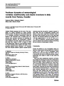
Figure 1.  Real observations and SVM results for (a) AT, (b) RH, (c) SLP, (d) SST, (e) WS, (f) evaporation estimated based on real observations and on forecasts.

3291

observations (year 1  + year 2). Furthermore, all data were scaled in the interval [0.1, 0.9] in order to avoid scaling problems during SVM ­computations. All PSO simulations involved 20 particles and 1000 as maximum number of iterations. SVM and PSO were run on a computer with Intel Core i7 2.20 GHz processor and 8 GB of RAM on a 64 bits Linux operating system. The SVM parameters found by PSO related to each of the five analyzed time series are shown in Table 2. Note that these values are associated with second differenced and scaled data. Figure  1a–e depicts the daily real observations along with SVM forecasts for AT, RH, SLP, SST and WS, respectively, as well as the corresponding MAE values. From a visual inspection of Figure 1a–e, it can be noticed that he SVM combined with the prediction procedure described in Section  4 is able to catch the behavior of each environmental indicator. For the sake of illustration, from the predicted values of AT, SLP, SST and WS, one can estimate a year-ahead of daily evaporation (E, in g/m2.s) from the bulk formula (Katsaros, 2001):

of environmental indicators monitored by the PIRATA Project. The obtained predictions matched the general real behavior of each considered variable (AT, RH, SLP, SST and WS). This fact along with the obtained MAE values suggests that the methodology proposed by Lins et al. (2013) is a promising tool in the prediction of meteorological variables. The estimation of a year-ahead daily evaporation was obtained by means of the predictions of AT, SLP, SST and WS. This illustrates how an indirectly measured environmental indicator can be obtained based on forecasts of other variables. Given that surface meteorological variables are essential to anticipate the occurrence of hazardous natural events, this paper can be part of a more general environmental/social risk framework. The anticipation of such events enable the implementation of appropriate actions in order to reduce or avoid the related undesired consequences.

E = ρ CE WS (qs - q),

Aguilar-Martinez, S. & Hsieh, W.W. 2009. Forecasts of Tropical Pacific sea surface temperatures by neural networks and support vector regression. International Journal of Oceanography, 2009. Article ID 167239, 13 pages, doi:10.1155/2009/167239. Bolton, D. 1980. The computation of equivalent potential temperature. Monthly Weather Review, 108: 1046–1053. Bourlès, B., Lumpkin, R., McPhaden, M.J., Hernandez, F., Nobre, P., Campos, E., Yu, L., Planton, S., Busalacchi, A., Moura, A.D., Servain, J. & Trotte, J. 2008. The PIRATA program: hystory, accomplishments and future directions. Bulletin of the American Meteorological Society, 89(8): 1111–1125. Boyd, S. & Vandenberghe, L. 2004. Convex optimization. Cambridge: Cambridge University Press. Brockwell, P.J. & Davis, R.A. 2002. Introduction to time series and forecasting. New York: Springer-Verlag. Burges, C.J.C. 1998. A tutorial on support vector machines for pattern recognition. Norwell, MA: Kluwer. Chatfield, C. 2004. The analysis of time series: An ­introduction. Boca Raton: Chapman & Hall/CRC. Hsu, C.-W., Chang, C.-C. & Lin, C.-J. 2003. Last updated: april/2010. A practical guide to support vector classification. Department of Computer Science, National Taiwan University. Katsaros, K. 2001. Evaporation and humidity. In J. Steele, S. Thorpe & K. Turekian (eds.), Encyclopedia of Ocean Sciences: 870–877. Academic Press. Kecman, V. 2005. Support vector machines: an ­introduction. In L. Wang (ed.), Studies in Fuzziness and Soft Computing: 1–47. Berlin Heidelberg: Springer-Verlag. Lin, H.-T. & Lin, C.-J. 2003. A study on sigmoid kernels for SVM and the training of non-PSD kernels by SMO-type methods. Department of Computer Science and Information Engineering, National Taiwan University.

(12)

where ρ is the air density (in kg/m3), CE is the exchange coefficient for water vapor. The air density is considered as ρ  =  1.2  kg/m3 for the location 10°S 10°W and CE = 0.0011 (Katsaros, 2001). Also, in Equation (12), qs is the saturation specific humidity at the air-sea interface and q is the specific humidity, which are given by (in g/kg): q(s) = 0.622 es 1000/(SLP - es),

(13)

where es is the saturation vapor pressure (in hPa) and is a function of the temperature (τ). For the calculation of qs, τ  =  SST and for the computation of q, τ = AT in the following formula (Bolton, 1980): es = 6,112 exp[17.67 τ/(τ + 243.5)].

(14)

Figure 1f presents the daily evaporation for the period 17-Sep-2010 to 16-Sep-2011 calculated with real observations of AT, SLP, SST and WS and also with the corresponding forecasts. The estimates based on predicted values presented a similar behavior when compared against the estimates based on real values. The associated MAE is also provided in Figure 1f. 7  Conclusion This paper used an SVM combined with a yearahead prediction procedure to provide ­forecasts

References

3292

Lins, I.D., Araujo, M., Moura, M.C., Silva, M.A. & Droguett, E.L. 2013. Prediction of sea surface temperature in the tropical Atlantic by support vector machines. Computational Statistics and Data Analysis, 61: 187–198. Lins, I.D., Moura, M.C. & Droguett, E.L. 2010a. ­Support vector machines and particle swarm optimization: ­applications to reliability prediction. Saarbrücken, Germany: Lambert Academic Publishing. Lins, I.D., Moura, M.C., Silva, M.A., Droguett, E.L., Veleda, D., Araujo, M. & Jacinto, C.M. 2010b. Sea surface temperature prediction via support vector machines combined with particle swarm optimization. In 10th International Probabilistic Safety Assessment and Management Conference—PSAM 10, Seattle, WA, EUA, 7–11 June 2010. Moura, M.C., Lins, I.D., Veleda, D., Droguett, E.L. & Araujo, M. 2010. Sea level prediction by support vector machines combined with particle swarm optimization. In 10th International Probabilistic Safety Assessment and Management Conference—PSAM 10, Seattle, WA, EUA, 7–11 June 2010. Nougier, J.P. 1993. Méthodes de calcul numérique. Paris: Masson. Schölkopf, B. & Smola, A.J. 2002. Learning with kernels: support vector machines, regularization, optimization, and beyond. Cambridge, MA: The MIT Press.

Servain, J., Busalacchi, A., McPhaden, M.J., Moura, A.D., Reverdin, G., Vianna, M. & Zebiak, S. 1998. A pilot research moored array in the tropical Atlantic (PIRATA). Bulletin of the American Meteorological Society, 79: 2019–2031. Shölkopf, B. & Smola, A.J. 2002. Learning with kernels: support vector machines, regularization, optimization and beyond. Cambridge: The MIT Press. Sorjamaa, A., Hao, J., Reyhani, N., Ji, Y. & Lendasse, A. 2007. Methodology for long-term prediction of time series. Neurocomputing, 70: 2861–2869. Vapnik, V.N. 2000. The nature of statistical learning theory. New York: Springer-Verlag. Wu, A., Hsieh, W.W. & Tang, B. 2006. Neural network forecasts of the Tropical Pacific sea surface temperatures. Neural Networks, 19: 145–154. Xie, S.-P. 2007. Ocean-atmosphere interaction and tropical climate. In Y. Wang (ed.), Encyclopedia of Life Support Systems (EOLSS)—Tropical Meteorology: 870–877. Xie, S.-P. & Philander, G.H. 1994. A coupled ocean­atmosphere model of relevance to the ITCZ in the eastern Pacific. Tellus, 46A: 340–350.

3293