RESEARCH ARTICLE
Adv. Sci. Lett. 21, 3079–3083, 2015
Copyright © 2015 American Scientific Publishers All rights reserved Printed in the United States of America
Advanced Science Letters Vol. 21, 3079–3083, 2015
PREDICTION OF CO2 EMISSIONS USING AN ARTIFICIAL NEURAL NETWORK: THE CASE OF THE SUGAR INDUSTRY Chairul Saleh1, Raden Achmad Chairdino Leuveano2, Mohd Nizam Ab Rahman3, Baba Md Deros4, Nur Rachman Dzakiyullah5 1Department
of Industrial Engineering, Faculty of Industrial Technology, Universitas Islam Indonesia, Yogyakarta, Indonesia of Mechanical and Material Engineering, Faculty of Engineering and Build Environment, Univeriti Kebangsaan Malaysia, Malaysia 5Department of Informatics Engineering, Faculty of Business and Information Technology, University of Technology Yogyakarta, Indonesia
2,3,4Department
In this paper, the back-propagation artificial neural networks (ANN) model is presented to predict expenditure of carbon (CO2) emission. The model was built based on the input variables that affect to expenditure of CO 2 include the amount of bagasse, wood and marine fuel oil used in boiler machine. The objective of this paper is to monitor the CO 2 emission based on the fuel used for operating the boiler machine. The data used for testing the models were obtained from Sugar Industry. It splits up into 90% of training data and 10% of testing data. The model experiment was conducted using trial and error approach to find the optimal parameters of ANN model. The result shows that the architecture of ANN model have optimal parameter on training cycle 50, learning rate 0.1, momentum 0.1, and 19 hidden nodes. The validity of the trained ANN is evaluated by using Root Mean Square Error (RMSE) with error value as 0.055. It indicates that the smallest error provides more accurate results on prediction and even can contribute to the industrial practice, especially helping the executive manager to make an effective decision for business operation by considering the expenditure of CO2 monitoring. Keywords: Artificial Neural Network, prediction, carbon emission, RMSE.
1. INTRODUCTION The global warming effect poses a significant threat to the environment. According to Research Working Group III of the Intergovernmental Panel on Climate Change (IPPC), a variety of living creatures, including humans, are the highest producers of greenhouse gases causing global warming1. Greenhouse gases such as carbon dioxide, methane and nitrous oxide act as a blanket layer in the Earth’s atmosphere, trapping the sun’s heat and increasing the temperature of the Earth. As stated in the fourth assessment report from the IPCC2, fossil fuels used by human activities in the energy sector, transportation, agriculture and industry have been linked to the increase in greenhouse gases. *
Email Address:
[email protected]
3079
As a key sector of production and the backbone of the economy in Indonesia, the manufacturing industry contributed 118.12 MtCO2 in 20113. From these data, it is apparent that large volumes of energy are consumed to produce goods or services within the economy, but also wastes are generated from such production operations. As a result, there will be a continuous increase in CO2 emissions, categorized as air waste/pollutants. Therefore, the Indonesian government needs to address this by controlling industries’ emissions. As one of the large contributors to CO2 emissions, the sugar industry is here selected as a case study. In 2008, 3.92 million tonnes of sugar was produced in Indonesia4. The more sugar produced, the more CO2 emissions are potentially generated. These emissions can come from the fuel used in boilers and the consumption of electricity, solar energy and liquid petroleum gas (LPG). For instance,
Adv. Sci. Lett. Vol. 21, No. 3079-3083, 2015
doi:10.1166/asl.2015.64881
RESEARCH ARTICLE
Adv. Sci. Lett. 21, 3079–3083, 2015 boilers are fired by fuel to generate steam. This steam then used to produce electricity using a generator to change the energy from heat to mechanical energy. The electricity produced by the boiler is then used to operate the cane cutter and hammer shredder to crush the sugar cane in the first stage of the process. The combustion of fuel in the boiler emits CO2, potentially generating air pollutants. This relationship between polluting emissions and energy consumption has been studied by Pao and Tsai5. It is necessary to monitor machines in industrial operations as each machine can contribute different amount of emissions. As boilers depend on fuel combustion, potentially high in emissions, this study focuses on boilers and investigates the variables that affect CO2 emissions from these machines. The three types of fuel used to operate boilers include bagasse (fibrous sugarcane residue), firewood and marine fuel oil (MFO). Monitoring these fuels is very important because they have different effects on the emission of CO2. To monitor machine emissions, most studies use regression, discriminant analysis and artificial neural networks (ANN) in empirical modelling to control the system6,7,8. Of these, the ANN model has proved the most attractive to researchers for predicting the behaviour of a system in certain cases and neural networks have increasing been used in recent years over conventional statistical techniques such as regression and discriminant analysis9. The model includes machine performance testing, cutting mechanics, signal processing, data decomposition and image processing10. The ANN model is a statistical learning algorithm, the design of which was inspired by the properties of biological neural systems, used to search and produce new knowledge to estimate functions based on a large number of inputs11. The ANN model can also be defined as a mathematical model for predicting new problems12. As harmful emissions have increased, previous research has also attempted to embed the use of ANNs in environmental applications. Baareh13 applied the ANN model to estimate CO2 emissions for consumption from four fuel inputs, including global oil, natural gas (NG), coal and primary energy (PE). Fontes et al14 employed ANN model to classify ozone episodes, which have a negative impact on the environment. This aimed to reduce inefficiency leading to ozone precursor emissions. To prevent fouling problems in machines resulting in higher CO2 emissions, Romeo and Gareta15 and Rusinowski and Stanek16 used the ANN method to monitor boiler performance. As the ANN model is a powerful tool for handling such types of modelling processes, this paper proposes an ANN model to predict CO2 emissions in boilers in the sugar industry. The objective is to monitor CO2 emissions based on fuel combustion used to operate the boilers in sugar production. By monitoring the machines, the sugar industry can efficiently manage fuel combustion. The remainder of this paper is organized as follows: section 2 introduces the materials and methods in the design of the ANN model; section 3 presents the result of the experiment; finally, section 4 summarizes the salient points and concludes the paper.
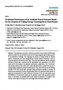
2. MATERIALS AND METHODS To design the ANN model for predicting the CO2 emissions from boiler use, a number of steps were defined as shown in Fig. 1.
Data collection Bagasse Firewood MFO Carbon emission
Dataset cleansing, transformation-normalization k-fold cross-validation Total Data 1 2
Cross-validation
.. 10
Training Set
Test Set
Model Search
Model evaluation Fig. 1. Design overview of the ANN model.
The first step to in the design of the ANN model is data collection. The primary data were collected from the sugar industry in Yogyakarta. This research analyses boiler emissions based on the fuel used. The three main fuels that affect CO2 emissions are found to include bagasse, firewood and MFO. These fuels are thus categorized as input variables. The output variable (CO2 emission) is computed by multiplying activity data (e.g. fuel consumed) by the emission factor for that activity, in accordance with the guidelines for computation of emissions provided by the IPCC17. The relationship between the input and output variables is defined as:
Xi
Bagasse, X 1 Firewood , X 2 , Y
Adv. Sci. Lett. Vol. 21, No. 3079-3083 , 201 5
CO2
(1)
MFO, X 3 3080
RESEARCH ARTICLE
Adv. Sci. Lett. 21, 3079–3083, 2015
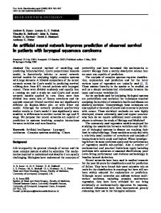
To avoid any noisy data, missing data, incorrect, improperly formatted, or duplicated in datasets, then data cleansing is employed18. The aim of data cleansing is to have a better representative datasets for developing reliable neural network model and improve the accuracy of prediction. The process of data cleansing in this study was automatically performed by Rapid Miner software. However, as shown in Fig. 2, the cleansing process shows that dataset has zero noisy and missing value. The next step is to transform and normalize the dataset in order to have inputs with 0 means and a standard deviation of 1.
A back-propagation (BP) learning algorithm is then used in the training process to obtain the optimal parameters. BP training is categorized as a gradient descent algorithm7. With this technique, the total error can be reduced by changing the weight along its gradient. However, to analyse the effect of network parameter, a trial and error approach is used in the design of the BP neural network prediction by varying the network structure based on the pre-processing of the data, the number of input nodes and the activation function. To evaluate the model error, the root mean square error (RMSE) is expressed by:
RMSE
1 2
1/2
Y jk j
O jk
(2)
k
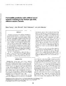
where Y is the predicted value and O denotes the actual value vectors over pattern k. 3. RESULTS Fig. 2. The process of data cleansing using Rapid Miner Then, to validate the model, k-fold cross-validation is used. This technique divides the dataset into a training set and a test set. The training set is used to calculate the gradient and update the network weights and biases. In this case, validation was computed during the training process to obtain minimum error in prediction. The test dataset is used to assess the performance of a fully-trained ANN model with data outside the training set. To find the optimal architecture of the ANN model in the training process, the parameters – training cycle, learning rate, momentum and hidden node – must be optimal. The simplified architecture of the ANN model comprising three layers (input variables, hidden nodes and output variable) is shown in Fig. 3.
Rapid Miner 5.2.003 was to carry out the experiment. All the test problems were undertaken using a computer with the following specifications: Intel (R) Core (TM) i52450M CPU @ 2.50GHz (4 CPUs), 8 GB of RAM and Windows 8.1, 64-bit (6.3, Build 9600) operating system. As mentioned previously, the data for the experiment were obtained from the sugar industry in Yogyakarta, Indonesia. There are 124 datasets for the period 2009–2013 on the use of fuels, including bagasse (tonnes), firewood (tonnes) and MFO (litres), for boiler operation. From the data on fuel consumed, the next step is to calculate the CO2 emissions (tonnes CO2) using the IPCC17 (2006) guidelines. Our objective is to monitor CO2 emissions from boilers, seek an accurate prediction that has the lowest error. In other words, an accurate prediction can provide information regarding the fuel consumption that has the lowest emissions. In this experiment, 10-fold cross-validation was used to split the data into a training set and a test set. The data were divided into 10 sets of size n/10 or equal parts: 90% of the data were used for the training set and 10% for the testing set. Error evaluation was then performed on 90/10 splits, repeated for all 10 possible splits. For each repetition, the training fold was normalized. The mean values and standard deviations were taken over k different partitions. The k-fold cross-validation technique was used as it can provide a lower variance, meaning that minimum error can be achieved. As noted above, the ANN model consists of three layers, for which the parameters include the training cycle, the learning rate, momentum and hidden nodes. Using the BP algorithm with a trial and error approach for the training process, the optimal architecture of the ANN model is as shown in Table 1.
Fig. 3. Simplified architecture of the ANN model 3081
Adv. Sci. Lett. Vol. 21, No. 3079-3083 , 201 5
1
RESEARCH ARTICLE
Adv. Sci. Lett. 21, 3079–3083, 2015 Table 1. Optimal parameters of the back-propagation ANN model Parameters Value Training Cycle Learning Rate Momentum Hidden Nodes RMSE
50 0.1 0.1 19 0.055
The objective of the training process is to minimize the error of prediction. This is taken as a rule to choose the optimal parameters of the ANN model. As can be seen from Table 1, the performance of the ANN model has an error value (RMSE) of 0.055. The closer the error value is to zero, the higher the accuracy of prediction. When the error value achieved its minimum, the training cycle was terminated at 50 cycles. The learning rate of the ANN model was 0.1. The value of the learning rate represents the speed at which the system learns (converges). The momentum rate has the same value as the learning rate, which is 0.1. The momentum rate is used to avoid local minima and significant changes in weights so that the global minimum can be achieved. The optimal hidden nodes in the network numbered 19. Determining the optimal number of hidden nodes can avoid overfitting and underfitting of the model. Overfitting occurs when the learning algorithm captures noise from the data, whereas underfitting occurs when the learning algorithm cannot correctly detect the underlying trend of the data, so that the model shows low bias but high variance. Based on the results of the experiment, Fig. 4 shows the actual and predicted values for both training and test cases.
In the last step, the model output of the neural network is analysed. This analysis aims to determine the level of confidence in the trained model by seeing whether the predicted values are normally distributed19. If the predicted value is normally distributed, the model prediction has higher accuracy and precision. Several statistical tests can be employed to check the normality of distribution, including the Shapiro–Wilk test, the Lilliefors test, D’Agostino–Pearson’s L2 test, the Jarque–Bera test, and the Anderson–Darling test. However, the most applicable statistical method that fits all types of distribution and sample size is the Shapiro–Wilk test20 and thus it was used in this study to test normality. In this paper, the significance level (α) was set at 0.05; if p