Prediction of Contact Maps Using Support Vector Machines

Prediction of Contact Maps Using Support Vector Machines

Technical Report

Department of Computer Science and Engineering University of Minnesota 4-192 EECS Building 200 Union Street SE Minneapolis, MN 55455-0159 USA

TR 02-039 Prediction of Contact Maps Using Support Vector Machines Ying Zhao and George Karypis

December 09, 2002

Prediction of Contact Maps Using Support Vector Machines∗ Ying Zhao and George Karypis Department of Computer Science, University of Minnesota, Minneapolis, MN 55455 {yzhao, karypis}@cs.umn.edu Abstract Contact map prediction is of great interests for its application in fold recognition and protein 3D structure determination. In particular, we focusd on predicting non-local interactions in this paper. We employed Support Vector Machines (SVMs) as the machine learning tool and incorporated AAindex to extract correlated mutation analysis (CMA) and sequence profile (SP) features. In addition, we evaluated the effectiveness of different features for various fold classes. On average, our predictor achieved an prediction accuracy of 0.2238 with an improvement over a random predictor of a factor 11.7, which is better than reported studies. Our study showed that predicted secondary structure features play an important roles for the proteins containing beta structures. Models based on secondary structure features and CMA features produce different sets of predictions. Our study also suggests that models learned separately for different protein fold families may achieve better performance than a unified model.

1

Introduction

Proteins are the molecular devices of life. They are the molecules that regulate the vital fluxes of mass and energy in biological systems. With the continued completion of genome projects their sequences become known at an everincreasing rate. The determination of the structure of proteins is deemed as a key step toward understanding the behavior of proteins and initiating knowledge-based, rational approaches for engineering molecular solutions. Experimental efforts, such as x-ray crystallography and NMR techniques are not efficient enough to allow for rapid structural determination of the ever increasing number of newly discovered sequences. Hence, computational, theoretical methodologies are becoming the sine qua non of protein sequence/structure/function relationship research. Although the mechanism of protein folding is not yet generally known, it can be reasonably assumed that non-local interactions are necessary for secondary structural elements to result in a cohesive native structure, which is favored energetically over alternative conformations. Whereas local interactions are responsible for secondary structural characteristics, non-local interactions are crucial for proteins to attain their native state. Numerous experimental and theoretical studies have demonstrated this importance of non-local interactions in foldability, as protein fold attainment is commonly referred to [17, 1, 8]. Furthermore, and besides the foldability, non-local interactions are important for maintaining the stability and hence the functionality of proteins [7, 15]. Site-directed mutagenesis experiments have amply demonstrated this importance [27, 13, 24]. Hence, the prediction of non-local interactions is of great interests for its use in protein fold recognition and 3D structure recovery. Specifically, identifying pairs of non-sequential amino acid residues or secondary structural elements that interact in 3D space provides a set of topological constraints that can be utilized in protein fold recognition. Nevertheless, if the contacts of a protein are known, its 3D structure can be deduced from its contact map [31]. Over the years, a variety of different approaches have been developed for contact map prediction [6, 18, 28, 32, 21], in which various machine learning tools as well as various features have been employed. The various learning mechanisms include Neural Networks [6, 21], statistical approaches based on correlated mutation [18, 28], and association ∗ This work was supported by NSF CCR-9972519, EIA-9986042, ACI-9982274, ACI-0133464, by Army Research Office contract DA/DAAG55-98-1-0441, by the DOE ASCI program, and by Army High Performance Computing Research Center contract number DAAH04-95C-0008. Related papers are available via WWW at URL: http://www.cs.umn.edu/˜karypis

1

rule based classification [32]. Whereas, the various features include sequence profiles derived from multiple sequence alignment [6, 32, 21], correlated mutation [6, 18, 28], predicted secondary structures [6, 21] and folding initiation sites (I-sites) [32]. However, the accuracy of contact map prediction is still far from satisfactory. The current stateof-art contact map predictor reported at CASP4 achieved an avarge accuracy of 0.21 (a 6-fold improvement over a random predictor). One of the interesting outcomes of previous research has been the observation that adding predicted secondary structure information is very helpful for contact map predictions [21, 6], even more useful than sequence profiles [21]. However, all previous approaches did not differentiate proteins of different fold families, i.e., the importance of various features was studies based on their performance on all proteins from different fold families. On the other hand, Reva and Topiol [26] recently found that beta-structures contribute more significantly to fold recognition than alphastructures, which raises the question whether beta-structures also contribute more significantly than alpha-structures to contact map prediction. The available knowledge of protein fold families (CATH [19]) enables us to answer this question by testing the effectiveness of predicted secondary structures in contact map prediction for various protein fold families. Especially, we focused on the class level from CATH [19] and tested whether the predicted secondary structure features are equally important for proteins with mainly alpha-structures, mainly beta-structures, and both alpha and beta structures. Furthermore, we would like to address an even broader problem, i.e., for the various fold classes, how effectively the different features (i.e., correlated mutation, sequence profiles and predicted secondary structures) predict contact maps. In addition, we employed Support Vector Machine (SVM) as the classification tool and incorporated AAindex [12] to extract correlated mutation and sequence profile features. On average, our predictor achieved a prediction accuracy of 0.2238 with an improvement over a random predictor of a factor 11.7, which is better than reported studies. Our study showed that predicted secondary structure features play an important roles for the proteins containing beta structures. Models based on secondary structure features and CMA features produce different sets of predictions. Our study also suggests that models learned separately for different protein fold families may achieve better performance than a unified model. The rest of this paper is organized as follows. Section 2 provides some information on contact maps, non-local interactions, CATH and Support Vector Machines (SVMs). Section 3 describes our approach of predicting contact maps, including the features and models we studied. Section 4 provides the detailed experimental evaluation of various models for different protein fold groups and length groups. Section 5 discusses some important observations from the experimental results. Finally, Section 6 provides some concluding remarks.

2

Background Material

2.1 Contact Maps Contact maps are two-dimensional, binary representations of protein structures. For a protein with N residues, the contact map for each pair of amino acids k and l, (1 ≤ k, l ≤ N ), will have a value C(k, l) = 1, if a suitably defined distance d(k, l) < dthr , where dthr is a user-defined threshold distance between the amino acids, and C(k, l) = 0 otherwise. Appropriate distances between amino acid residues can be, for example, the one between the center of mass, the C α atoms, or the minimum one. A contact map is simply a convenient binary representation of a distance matrix D, defined as D = [|rkl |], where |rkl | is the distance between the residues k and l. A particular cutoff distance, dthr , is chosen and we assign C(k, l) = 1 for all D(k, l) < dthr . In principle, contact maps can be built for alternative unit geometrical objects. For instance, contact maps can be created for pairs of secondary structural elements instead of residues, creating a more coarse-grained representation of the protein structure. In our study, we adopted the definition ˚ of distances to be the distances between the C α atoms of two amino acids and the distance threshold to be 8 A.

2.2 Non-local Contacts In our study, we focused on the off-diagnol regions of the contact maps, (i.e., non-local contacts). Consider a protein sequence [a1 , a2 , . . . , a N ] where N is the number of amino acid residues. We define as non-local any pairwise interactions between amino acids ai and a j with the sequence separation |i − j| > 6. Interactions between amino acids with sequence separations |i − j| ≤ 6 we define as local, including intra-loop and intra-helix interactions between any residues i and i + 5. Non-local interactions are necessary for protein secondary structural elements to result in a cohesive native structure, which is favored energetically over alternative conformations. The significance of non-local interactions in the foldability, the stability, and the functionality of protein molecules results in a distinct signature of amino acid residue conservation and covariation during evolutionary processes. 2

2.3 CATH Currently, CATH [19] and SCOP [16] are the major repositories of classified protein structures. CATH stands for Class, Architecture, Topology, and Homologous superfamily, the four levels of protein hierarchical classification used. The secondary structure elements and their packing are used to determine the Class. The Architecture level describes the global shape of the protein incorporating the orientation of secondary structure elements, but ignoring the specific connectivities. In the level of Topology, proteins are grouped based on shape and connectivity. Finally, sets of protein folds are grouped depending on their evolutionary relationships. More recently, a protocol was developed that integrates gene sequences from GenBank [2] within the CATH database, resulting in a significant expansion of the database to 176,597 domain sequences [20]. Class is determined according to the secondary structure composition and packing within the structure. It can be assigned automatically for over 90% of the known structures using the method of Michie et al. (1996). For the remainder, manual inspection is used and where necessary information from the literature taken into account. Three major classes are recognized; mainly-alpha, mainly-beta and alpha-beta. This last class (alpha-beta) includes both alternating alpha/beta structures and alpha+beta structures, as originally defined by Levitt and Chothia (1976). A fourth class is also identified which contains protein domains which have low secondary structure content. In our study, we focusd on the class level only, i.e., we differentiated the proteins by the types of their secondary structure elements.

2.4 Support Vector Machines Support vector machines is a state-of-the-art classification technique based on pioneering work done by Vapnik et al, [30]. This algorithm is introduced to solve two-class pattern recognition problems using the Structural Risk Minimization principle [30]. Given a training set in a vector space, this method finds the best decision hyperplane that separates two classes. The quality of a decision hyperplane is determined by the distance (referred as margin) between two hyperplanes that are parallel to the decision hyperplane and touch the closest data points of each class. The best decision hyperplane is the one with the maximum margin. By defining the hyperplane in this fashion, SVM is able to generalize to unseen instances quite effectively. The SVM problem can be solved using quadratic programming techniques [30]. SVM extends its applicability on the linearly non-separable data sets by either using soft margin hyperplanes, or by mapping the original data vectors into a higher dimensional space in which the data points are linearly separable. The mapping to higher dimensional spaces is done using appropriate kernel functions, resulting in efficient algorithms. A new example is classified by representing the point the feature space and computing its distance from the hyperplane. SVM (Support Vector Machine) has been applied to a wide range of classification problems because of its many attractive features, including effective avoidance of overfitting, and the ability to handle large feature spaces. The success of SVM has been showed in documents classification [4] and secondary structure predictions [9].

3

Contact Map Prediction

The problem of contact map prediction can be stated as a classification problem. Given a set of proteins with known structures, contact residues and non-contact residues are separated as positive instances and negative instances. For each instance, various features are collected to capture useful information of the pair of residues, including amino acid content, physicochemical environment, secondary structures, evolutionary correlation, and other information that can discriminate contacts from non-contacts. Then, these feature vectors of both positive instances and negative instances are used as the input to a classification tool to learn a classifier (i.e., predictor). Given a sequence with unknown structures, the resulting predictor classifies the pairs of residues of the sequence to be contacts and non-contacts based on their feature vectors. In our approach, we employed Support Vector Machines (SVMs) as the classification tool and collected various features based on primary sequences, multiple sequence alignments, predicted secondary structures and correlated mutation analysis. For the rest of this section, we will describe in detail how we extracted various features and designed learning models. Correlated Mutations Analysis (CMA) and Sequence Conservation A variety of correlated mutations analysis (CMA) tools have been proposed to predict non-local contacts [18, 22, 23, 25, 6]. The correlated mutations analysis (CMA) utilizes evolutionary information. In evolutionary times, the significance of non-local contacts is manifested in the observed conservation patterns and the covariation of amino acid residues in multiple sequence alignments of homologous proteins. Pairs of distant sequence positions that are 3

proximal in three-dimensional space appear to be conserved or mutated in a correlated fashion, i.e. the frequencies of particular amino acid appearances in one position are dependent on the amino acid residue in the other position. In principle, positions with high correlation coefficients, a quantitative measure of mutational covariance in families of homologous proteins, can be inferred to be proximal in 3D. Instead of following the simple employment of a few physicochemical vectors, such as the volume or the hydrophobicity, as was done in previous literature work, we used the ten first principal components that resulted from a principal component analysis on 142 physicochemical vectors in AAindex, a database of published amino acid properties [12]. Given a multiple sequence alignment (MSA) of a protein, for each pair of amino acids of the protein, the extent of covariation in mutations was calculated using a simple correlation coefficient ri j =

1 NM S A2

NX MSA

(qil − m i )(q lj − m j ) si s j

l=1

,

(1)

where qil and q lj are the values for some amino acid physicochemical vector (volume, hydrophobicity, etc.) for sequence l at positions i and j. m i , m j , si and s j are the mean values and the standard deviations of the amino acid properties at i and j. The sum runs over all the N M S A sequences in the multiple sequence alignment. We also calculated correlated mutations defined in [18], which also employed similar correlation coefficient measure, but used pairwise amino acid scoring matrix of McLachlan [14] instead of physicochemical vectors. The positions that are completely conserved or contain more than 10% gaps in MSAs are not included for CMA calculation. The conservation of each position in the sequence is also calculated based on the Entropy value of the amino acids appearing at the position in the multiple sequence alignment as follows,

Con(i) = −

20 X

P(ak |i) log P(ak |i)

(2)

k=1

where ak is one of the 20 amino acids and P(ak |i) equals the number of sequences containing ak at the position i divided by the total number the sequences in the multiple sequence alignment. Features For each pair of positions in a protein sequence, we identified five sets of features that capture different aspects of the amino acids and the locations i and j: sequence conservation (Con), sequence separation (Sep), correlated mutations analysis (CMA), predicted secondary structures (PSS) and sequence profiles (SP). Sequence Conservation (Con) Sequence conservation values based on multiple sequence alignment were calculated for positions i and j by using Equation 2. Sequence Separation (Sep) defined by |i − j|.

Sequence separation is the distance between two amino acids in the sequence and

Correlated Mutations Analysis (CMA) For positions i and j, we extracted three sets of Correlated Mutations Analysis (CMA) features. First, we calculated the correlated mutation value defined in [18] and refer this feature as CMA (McLachlan). Second, we used the ten first principal components that resulted from a principal component analysis on 142 physicochemical vectors in AAindex [12] as the property vectors. Then, for each one of ten vectors, we calculated the correlated mutation value by using Equation 1. We refer these ten features as CMA (PCA10). Finally, AAindex [12] provided a six-way clustering of all the 142 physicochemical vectors (alpha and turn propensities, beta propensity, Physicochemical properties, composition, hydrophobicity and other properties). From each cluster, five vectors were selected and used in correlated mutation calculation. We refer these 30 features as CMA (30). We also refer CMA to all the 41 correlated mutation analysis features. Predicted Secondary Structures (PSS) For each residue, we used three values to represent whether it belongs to an alpha helix, beta strand or coil. If the residue belongs to one of the three secondary structures, we set the corresponding value to be 1, and 0 otherwise. For each residue pair (i, j), we considered a window of width three,

4

(i.e., we considered positions i − 1, i, i + 1, j − 1, j, and j + 1). Hence, we have 18 secondary structure features in total. Sequence Profiles (SP) The use of sequence profiles, which are derived from a multiple sequence alignment of homologous sequences, have been shown to be able to improve the prediction of contact maps [6, 21]. We adopted the three-neighborhood approach in [6]. For positions i and j, the occurrence frequencies of all the possible amino acid pairs (210) were calculated from the multiple sequence alignment. Besides (i, j), we also calculated the profiles of (i − 1, j − 1), (i + 1, j + 1), (i − 1, j + 1) and (i + 1, j − 1) and we refer these 1050 (210 ∗ 5) features as SP (Amino Acids). In addition to using amino acid pair frequencies to represent the profile, we also used twelve physicochemical vectors from AAindex [12] to describe the physciochemical environment around positions i and j. Again, we considered a window of width three around i and j. For each position, the average of one physicochemical property was calculated by averaging the physicochemical property values for all the amino acid that appeared at that position in the multiple sequence alignment. We refer these 72 (12 ∗ 6) features as SP (AAindex) and all sequence profile related features (SP (Amino Acids) + SP (AAindex)) as SP. Models We trained 15 SVM models by using different sets of features. Table 1 shows various models and the set of features used in each model. Besides the features showed in the table 1, all the 15 models contain the sequence conservation (Con) features for positions i and j. The 15 models can be grouped into four sets, predicted secondary structure (PSS) based, CMA based, Sequence Profile (SP) based, and combined models. We evaluated the different ways of extracting CMA features and SP features by comparing the various CMA based models and SP based models. Finally, we combined the five sets of features (Con, Sep, PSS, CMA, and SP) in various ways to evaluate their effectiveness. Table 1: Features used in various models Secondary Structure based Model Features 1 PSS

2 3 4 5

CMA based CMA (McLachlan) CMA (PCA10) CMA (30) CMA

Sequence Profile based Model Features 6 SP (AAindex) 7 SP (Amino Acids) 8 SP

Model 9 10 11 12 13 14 15

Combined Features Sep + PSS Sep + CMA Sep + PSS + CMA PSS + SP CMA + SP PSS + CMA + SP Sep + PSS + CMA + SP

Support Vector Machine (SVM) Training We adopted a three-way across-validation process for training and testing each model. The dataset was divided into three subsets randomly, out of which the model was trained with two subsets as the training set and tested on the other subset as the testing set. The splitting of the dataset was the same for each one of the 15 models. Given a training set, the input for SVM training is a collection of feature vectors of all the position pairs from all the sequences in the training set. We call each feature vector as a instance. We also input the true class label (positive for contacts and negative for non-contacts) of each instance for SVM training. Since there are much more non-contacts than contacts, we randomly sampled non-contact instances, so that the number of contact instances and the number of non-contact instances are the same approximately. Again, the negative instance sampling is the same for each one of the 15 models. All the 15 models were trained using SV M light [10] with a linear kernel and the default C value. Prediction of Contacts Given a testing sequence, the input for a predictor (i.e., one of the 15 models) is also a collection of features vectors of all the position pairs from that sequence. The predictor will return a score for each instance. If we assign contact to be the positive class and non-contact to be the negative class, then the higher the score is, the more likely the pair of amino acids is in contact. Hence, the returned scores can be sorted into a list, from which the top pairs are predicted as contact points. Finally, the contacts can be predicted by either setting a value threshold or the number of predicted contacts.

5

4

Experimental Results

4.1 Data Preparation Dataset The dataset we use in training and testing our predictors contains 177 proteins with known 3D structure from Protein Data Bank (PDB [3]). The proteins whose chains are not interrupted and contain no more than two domains were selected. The list of proteins was further reduced to only contain the proteins with pairwise sequence identity lower than 25%. Finally, we excluded the proteins that have less than 15 homologous proteins returned by PSI-BLAST when searching against non-redundant protein database (NR). Multiple Sequence Alignment and Predicted Secondary Structure To obtain multiple sequence alignments (MSAs), we first collected homologous sequences for each protein by using PSI-BLAST searching against non-redundant protein database (NR). We used the default parameters of PSI-BLAST and only kept sequences with more than 20% and less than 80% sequence identity. Then, we used ClustalW [29] to generate the final MSAs of the target protein and its homologous sequences. The predicted secondary structures for each proteins were obtained by using PSIPRED [11], a two-stage neural network predictor based on the position specific scoring matrices generated by PSI-BLAST.

4.2 Experimental Methodology and Metrics Evaluation Metrics To compare the results with other approaches [6], we predict the top L p /2 pairs to be contact points, where L p is the length of the protein. This cutoff is also based on the fact that in general the number of contacts increases linearly with the length of the protein [18]. We evaluated the prediction by calculating the accuracy and the improvement over a random predictor. The accuracy of the prediction is defined by the ratio of the number of correct predictions and the total number of predictions,i.e., Acc =

Ncp Np

(3)

where Ncp is the number of correct predictions and N p is the total number of predictions, which is also equal to L p in our experiments. A random predictor will place contact pairs randomly on the list. Hence the accuracy of the top L p /2 pairs is equal to the accuracy of the overall list, i.e., the density of contacts of the proteins, which is defined as follows, R Acc =

Nc N

(4)

where N is the total number of amino acid pairs with sequence separation greater than 6, and Nc is the number of observed contacts. Finally, the improvement over a random predictor is defined by the ratio between Acc and R Acc. Methodology Recall from Section 3, each model was learned by using a three-way cross-validation. Each protein appeared in one and only one testing set. Hence, the prediction accuracies of all the proteins were obtained after the three-way crossvalidation process. Since we are interested in the difference of prediction effectiveness for proteins of different fold families, we grouped the proteins according to their CATH codes as well as their lengths. For example, the CATH1 group contains the proteins with CATH class code 1, (i.e., mainly-alpha class). Since the proteins may contain two domains, we have combinations of single CATH classes. For example, the CATH1 & CATH3 group contains the proteins that have two domains, of which one belongs to CATH class 1 and the other belongs to CATH class 3. The group Others contains the proteins of unknown CATH codes or CATH class codes other than 1, 2 and 3. Note that the CATH1, CATH2 and CATH3 group may also contain multi-domain proteins, in which cases, the different domains belong to the same CATH class. In total, we have three length groups (i.e., short, median and long), and six fold groups. Table 2 shows the average density of the proteins within each group. The numbers in parentheses are the number of proteins in each group.

6

Table 2: Statistics of the Density of Contacts for Various Protein Categories l < 100 (40) 100 < l < 300 (101) l > 300 (36)

CATH1 (34) 0.0211(13) 0.0141(18) 0.0088(3)

CATH2 (35) 0.0588(9) 0.0347(24) 0.0135(2)

CATH3 (75) 0.0517(13) 0.0229(43) 0.0099(19)

CATH1 & CATH3 (9) -(0) 0.0136(5) 0.0110(4)

CATH2 & CATH3 (6) -(0) 0.0178(4) 0.0107(2)

Others (18) 0.0728(5) 0.0190(7) 0.0100(6)

As shown from table 2, the CATH1 group, mainly-alpha class, has significantly lower average densities than the other groups. Whereas, the CATH2 groups, mainly-beta class, has the highest average densities.

4.3 Results Table 3 shows the average prediction accuracy and random improvement factor of various models for different fold groups, in which each row represents each model and each column corresponds to each fold group. The overall performance of each model is also included in the last column. The values in parentheses are the average improvement over a random predictor for the proteins within each fold group. For each fold group, the entries of the best performance are in bold face. A number of observations can be made from table 3. First, the overall best model is model 15, which achieved 0.2238 accuracy and performs 11.7 times better than a random predictor. Second, in general, model 9, model 11 and model 15 behaved very similarly. Model 9 is based only on sequence separation (Sep) and predicted secondary structure (PSS) features. By adding correlated mutation analysis (CMA) features, model 11 performed slightly better than model 9 on average. By adding both CMA and sequence profile (SP) features, model 15 achieved the best performance. Third, for the CATH1 group, model 13, which is based on CMA and SP features, produced the best prediction accuracy of 0.0657 and random improvement factor of 4.6, which are 26% and 58% better than model 9, respectively. On the other hand, for the rest of the fold groups, except the CATH3 group, model 9 performed the best. For the CATH3 group, model 15 produced the best prediction on average. Finally, model 14 and model 1 performed more than 40% worse than model 15 and model 9, respectively, whereas, model 5 and model 11 had similar performance, which suggests that the sequence separation is indeed an important feature to be used together with PSS features, but may not be very useful when combining with other features. Table 3: Average Prediction Accuracy and Random Improvement of Various Models for Different Fold Groups model PSS CMA (based)

SP (based) Combined

1 2 3 4 5 6 7 8 9 10 11 12 13 14 15

CATH1 0.0545(2.9) 0.0528(3.3) 0.0476(2.8) 0.0502(3.0) 0.0489(3.2) 0.0443(2.5) 0.0592(3.6) 0.0611(3.8) 0.0512(2.9) 0.0551(3.5) 0.0555(3.2) 0.0587(3.7) 0.0657(4.6) 0.0606(4.1) 0.0584(3.3)

CATH2 0.1504(3.9) 0.1304(3.6) 0.1120(2.9) 0.1088(2.9) 0.1256(3.4) 0.1009(2.5) 0.1277(3.4) 0.1278(3.4) 0.2302(6.8) 0.1193(3.4) 0.2200(6.5) 0.1656(4.3) 0.1580(4.3) 0.1823(5.0) 0.2236(6.5)

CATH3 0.2024(9.6) 0.0910(4.4) 0.0921(4.1) 0.0933(4.1) 0.0900(4.4) 0.0833(3.7) 0.1321(6.3) 0.1382(6.6) 0.2695(14.9) 0.0897(4.5) 0.2811(15.3) 0.2064(9.8) 0.1519(7.4) 0.2086(10.2) 0.2845(15.4)

CATH1 & CATH3 0.1547(12.6) 0.0990(8.2) 0.0719(5.7) 0.0632(5.0) 0.0958(7.9) 0.0485(4.0) 0.1105(8.8) 0.1172(9.5) 0.2913(24.1) 0.0995(8.2) 0.2678(22.4) 0.1631(13.4) 0.1315(10.7) 0.1963(15.9) 0.2804(23.4)

CATH2 & CATH3 0.1225(8.3) 0.0596(4.1) 0.0459(3.2) 0.0486(3.6) 0.0643(4.4) 0.0560(3.7) 0.0787(4.9) 0.0831(5.3) 0.3003(21.4) 0.0724(5.3) 0.2899(20.5) 0.1490(10.3) 0.1091(6.7) 0.1529(10.3) 0.2995(20.9)

Others 0.1435(6.4) 0.0804(3.3) 0.0832(3.6) 0.0737(2.5) 0.0730(2.5) 0.0494(2.1) 0.0741(3.5) 0.0711(3.7) 0.2356(13.7) 0.0894(4.6) 0.2300(13.0) 0.1223(6.4) 0.0830(3.8) 0.1212(5.9) 0.2336(13.4)

Overall 0.1523(6.9) 0.0897(4.1) 0.0839(3.6) 0.0830(3.5) 0.0868(3.9) 0.0731(3.1) 0.1083(5.0) 0.1114(5.2) 0.2182(11.5) 0.0888(4.3) 0.2198(11.5) 0.1570(7.4) 0.1269(6.0) 0.1633(7.9) 0.2238(11.7)

We also summarized detailed performance of model 15 for different fold groups and length groups in table 4, in which each row corresponds to each fold group and each column corresponds to each length group. The overall average prediction accuracy and random improvement of each length group can be found in the last row. Again, the values in parentheses are the average improvement over a random predictor. As shown in table 4, model 15 performed well for the CATH3, CATH1 & CATH3 and CATH2 & CATH3 group. For these groups, the overall performance is in the range of 0.2805-0.2995 and 15.4 − 23.4 times better than a random predictor. The best performance for CATH3 proteins may be due to the fact that the majority proteins in our dataset are CATH3 proteins (i.e., 75 out of 7

177). Model 15 also performed relatively well for CATH2 proteins with an average prediction accuracy of 0.2236 and an average random improvement factor of 6.5 overall. However, for CATH1 proteins, model 15 performed poorly, only 3.3 times better than a random predictor with an average prediction accuracy of 0.0584. Since we have similar number of CATH1 proteins and CATH2 proteins in our dataset, the significant performance difference must relate to some characteristics of each fold group. Another observation we can made from table 4 is that the prediction accuracy decreases as the sequence length increases. However, the decrease is within the range of 13%-16%, which is much less significant than the ones reported before [6, 32]. The relatively good performance for long proteins indicates that our model is more robust to the length of proteins than other approaches. Table 4: Average Prediction Accuracy and Random Improvement of Model 15 for Different Fold Groups and Length Groups CATH1 CATH2 CATH3 CATH1 & CATH3 CATH2 & CATH3 Others Overall

5

l < 100 0.0501(2.2) 0.2760(4.8) 0.3125(6.9) -(-) -(-) 0.2703(3.5) 0.2137(4.5)

100 < l < 300 0.0670(4.0) 0.2014(6.2) 0.2836(13.5) 0.3021(23.0) 0.3121(18.4) 0.2578(15.9) 0.2257(10.9)

l > 300 0.0426(4.0) 0.2531(18.4) 0.2664(26.0) 0.2532(23.8) 0.2744(25.8) 0.1747(18.6) 0.2297(22.2)

Overall 0.0584(3.3) 0.2236(6.5) 0.2845(15.4) 0.2804(23.4) 0.2995(20.9) 0.2336(13.4) 0.2238(11.7)

Discussion

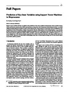
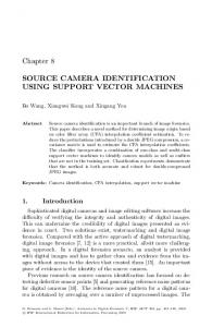
Different Fold Groups Prefer Different Sets of Features The most important observation from experimental results is that for different fold groups (e.g., CATH1, CATH2 and CATH3), the model that achieved the best performance is different. Predicted secondary structure (PSS) features performed the best for CATH2 but poorly for CATH1. On the other hand, correlated mutation analysis (CMA) and sequence profile (SP) features performed the best for CATH1 but poorly for CATH2. Finally, for CATH3, in which sequences contain both alpha structures and beta structures, the combined model (model 15) performed the best. For CATH2 proteins, a great proportion of the non-local contacts are the contacts within each beta sheet, which are closely related to the secondary structures. Hence, the predicted secondary structures contain very strong signals for identifying such non-local contacts and performed very effectively for CATH2 proteins. On the other hand, for CATH1 proteins, in which sequences contain mainly alpha structures, PSS features are less effective than CMA features and SP features, which indicates that the non-local contacts in CATH1 proteins are not greatly related to secondary structure of the residues in contact. In addition, the different performance of the various models also suggests that we can learn separate models for each fold class (mainly alpha, mainly beta, and alpha-beta), which may achieve better performance than a unified model. Since the state-of-art of the secondary structure prediction achieves an accuracy of 76%, it is feasible to first predict which CATH class the sequence is and than apply the corresponding predictor. Predicted Secondary Structure (PSS) Features and Correlated Mutation Analysis (CMA) Features Predict Different Sets of Contacts To further study the prediction ability of various features, we looked at the predictions of PSS and CMA features more closely. Figures 1 and 2 shows the true contact map, the contact map predicted by model 9 (PSS + Sep) and model 4 (CMA (30)) for protein 5pti and 3gatA, respectively. Note that the thin bands anti-parallel to the main diagonal in the contact map correspond to beta-sheets. As shown in both figures, clearly, PSS features and CMA features predict different sets of contacts. As we discussed before, the contacts within each beta sheet are closely related to the secondary structure, it is not surprised to see that PSS features discovered these non-local contacts effectively. On the other hand, CMA targets the problem from a different angle and utilizes the evolutionary information. Therefore, the predictions in general are not limited to be the non-local contacts within the same secondary structure. Since FSS and CMA features predict different sets of contacts, the next question is how we can combine these two types of features. The combined model (model 15) in our study was trained using SV M light [10] with a linear kernel. The resulting model was dominated by FSS features (Model 15 behaves similarly as model 9), which indicates that linear kernels are not able to combine these two types of features effectively and non-linear kernels are desired.

8

60

55

55

50

50

45

45

40

40

35

35

30

30

25

25

20

20

15

15

10

10

5

5

50

5

10

15

20

25

30

35

40

45

50

55

40

30

20

10

5

10

15

20

25

30

35

40

45

50

55

10

20

30

40

50

60

Figure 1: (a)true contact map for 5pti (b)contact map predicted by model 9 (c)contact map predicted by model 4 60

60

60

50

50

50

40

40

40

30

30

30

20

20

20

10

10

10

10

20

30

40

50

60

10

20

30

40

50

60

10

20

30

40

50

60

Figure 2: (a)true contact map for 3gatA (b)contact map predicted by model 9 (c)contact map predicted by model 4 Another possible reason is that that SV M light [10] optimizes the overall classification accuracy instead of the ranking of the instances. By adding more features, SV M light [10] is able to improve the overall classification accuracy. However, this improvement does not always translate to a better ranking of the instances. The Use of AAindex in correlated mutation analysis (CMA) and sequence profile (SP) Features As shown in table 3, model 2 (CMA (McLachlan)) performed the best among the CMA based models. Our attempts of incorporating AAindex in CMA did not improve the performance, which may be due to the fact that we included too many physicochemical vectors from various AAindex clusters. The prediction abilities of the vectors from different clusters may vary for various fold classes. Since we trained all the models using a linear kernel, the overall performance may be damaged by including all the various vectors. As for sequence profile (SP) features, although model 6 (SP (AAindex)) performed worse than model 7 (SP (Amino Acids), adding SP (AAindex) features (model 8) indeed improved the performance with a factor of 10% on average, which indicates that the average values of each physicochemical vector for a position contain useful information about the environment and can be used to improve predictions. Comparing to Other Approaches The comparison to previous reported results is in general difficult for contact map prediction for two reasons. First, previous studies adopted different definitions of the distance between two amino acids, contact threshold and the scope of contacts. For example, Fariselli et al. [6] focused on non-local contacts (|i − j| > 6), whereas, Pollastri and Baldi [21] considered all contacts without any sequence separation constraints. Since the scope of contacts influences the density of the contacts directly and the prediction of local contacts is quite different from non-local contacts, the direct comparison between the results of predicted contact maps with different scope is not fair. Second, average accuracy is not a good measure for it is influenced by the proportions of different length groups and fold groups. It will favor more short proteins and non-CATH1 proteins. However, we can still make relatively fair comparison to the results reported by Fariselli et al. [6, 5], the best contact map predictor reported at CASP4, because their dataset contains more short sequences and is “lack of representation of all-α proteins” [5]. They reported an average accuracy of 0.21 and with an improvement over random of a factor greater than 6. Whereas, our predictor achieved an average accuracy of 0.2238 with an improvement over a random predictor of a factor 11.7. Especially, our predictor achieved average accuracies of 0.2257 and 0.2297 with random improvement factors of 10.9 and 22.2 for median and long sequences, respectively. Our average accuracies are more than 20% and 100% better than those reported in [5] for median and long sequences, respectively, which indicates that our model can predict 9

long sequences more robustly.

6

Concluding Remarks

In this paper, we present our approach of predicting contact maps using support vector machines (SVMs). Our predictor achieved better results than those of previous approaches, especially for median and long sequences. We also evaluated the effectiveness of different features for various protein fold families. Our experimental results showed that different set of features achieved the best performance for various protein fold families, which directly leads to our future work. That is, learning models that are specific for each fold family. We also would like to adopt non-linear kernels to learn models that combine predicted secondary structure (PSS) features and correlated mutation analysis (CMA) features more effectively and develop filtering processes based on secondary structure constraints to further improve the accuracy of our predictors.

References [1] V. I. Abkevich, A. M. Gutin, and E. I. Shakhnovich. Impact of local and non-local interactions on thermodynamics and kinetics of protein folding. J. Mol. Biol., 252:460–471, 1995. [2] D. A. Benson, I. Karsch-Mizrachi, D. J. Lipman, J. Ostell, B. A. Rapp, and D. L. Wheeler. Genbank. Nucleic Acids Research, 28(1):15–18, 2000. [3] Helen M. Berman, T. N. Bhat, Philip E. Bourne, Zukang Feng, Gary Gilliland Helge Weissig, and John Westbrook. The Protein Data Bank and the challenge of structural genomics. Nature Structural Biology, 7:957–959, November 2000. [4] S.T. Dumais. Using svms for text categorization. IEEE Intelligent Systems Magazine, 13(4), 1998. [5] P. Fariselli, Olmea O., Valencia A., and Cassadio R. Progress in predicting inter-residue contacts of proteins with neural networks and correlated mutations. Proteins: Struct., Funct., Genet., Suppl 5:157–162, 2001. [6] P. Fariselli, Osvaldo Olmea, Alfonso Valencia, and Rita Casadio. Prediction of contact maps with neural networks and correlated mutations. Protein Eng., 14(11):835–843, 2001. [7] A. R. Fersht, A. Matouschek, and L. Serrano. The folding of an enzyme. i. theory of protein engineering analysis of stability and pathways of protein folding. J. Mol. Biol., 224:771–782, 1992. [8] D. Gilis and M. Rooman. Predicting protein stability changes upon mutation using database-derived potentials: solvent accessibility determines the importance of local versus non-local interactions along the sequence. J. Mol. Biol., 272:276–290, 1997. [9] S. Hua and Sun Z. A novel method of protein secondary structure prediction with high segment overlap measure: Support vector machine approach. J. Mol. Biol., 308:397–407, 2001. [10] T. Joachims. Making large-scale svm learning practical. Advances in Kernel Methods - Support Vector Learning, B. Schlkopf and C. Burges and A. Smola (ed.), MIT-Press, 1999, 1999. [11] David T. Jones. Genthreader: An efficient and reliable protein fold recognition method for genomic sequences. Journal of Molecular Biology, 287:797–815, 1999. [12] S. Kawashima, H. Ogata, and M. Kanehisa. AAindex: Amino acid index database. Nucleic Acids Research, 27:368–369, 1999. [13] J. T. Kellis, Jr., K. Nyberg, D. Sali, and A. R. Fersht. Contribution of hydrophobic interactions to protein stability. Nature, 333:784–786, 1988. [14] A. D. McLachlan. Test for comparing related aminoacid sequences. J. Mol. Biol., 61:409–424, 1971. [15] V. Mu˜noz and L. Serrano. Local versus nonlocal interactions in protein folding and stability-an experimentalist’s point of view. Folding & Design, 1:R71–77, 1996. [16] A. G. Murzin, S. E. Brenner, T. Hubbard, and C. Chothia. SCOP: a structural classification of proteins database for the investigation of sequences and structures. J. Mol. Biol., 247:536–540, 1995. [17] M. Niggemann and B. Steipe. Exploring local and non-local interactions for protein stability by structural motif engineering. J. Mol. Biol., 296:181–195, 2000. [18] O. Olmea, Burkhard Rost, and Alfonso Valencia. Effective use of sequence correlation and conservation in fold recognition. J. Mol. Biol., 293:1221–1239, 1999. [19] C. A. Orengo, A. D. Michie, S. Jones, D. T. Jones, M. B. Swindells, and J. M. Thornton. CATH—a hierarchic classification of protein domain structures. Structure, 5(8):1093–1108, 1997. [20] F. M. G. Pearl, D. Lee, J. E. Bray, I. Sillitoe, A. E. Todd, A. P. Harrison, J. M. Thornton, and C. A. Orengo. Assigning genomic sequences to CATH. Nucleic Acids Research, 28(1):277–282, 2000. [21] G. Pollastri and P. Baldi. Prediction of contact maps by recurrent neural network architectures and hidden context propagation from all four cardinal corners. Bioinformatics, 18 Suppl 1:S62–S70, 2002. [22] D. D. Pollock and W. R. Taylor. Effectiveness of correlation analysis in identifying protein residues undergoing correlated evolution. Protein Engineering, 10:647–657, 1997. [23] D. D. Pollock, W. R. Taylor, and N. Goldman. Coevolving protein residues: maximum likelihood identification and relationship to structure. J. Mol. Biol., 287:187–198, 1999. [24] M. Prevost, S. J. Wodak, B. Tidor, and M. Karplus. Contribution of the hydrophobic effect to protein stability: analysis based on simulations of the Ile-96—ala mutation in barnase. Proc. Natl. Acad. Sci., 88:10880–10884, 1991.

10

[25] P. Pritchard, Peter Bladon, Jane M. O. Mitchell, and Mark J. Dufton. Evaluation of a novel method for the identification of coevolving protein residues. Protein Eng., 14(8):549–555, 2001. [26] B. Reva and S. Topiol. Recognition of protein structure: Determining the relative energetic contributions of beta-strands, alpha-helices and loops. In Proc. of The Pacific Symposium on Biocomputing, pages 165–175, 2000. [27] L. Serrano, J. T. Kellis, Jr., P. Cann, A. Matouschek, and A. R. Fersht. The folding of an enzyme. ii. substructure of barnase and the contribution of different interactions to protein stability. J. Mol. Biol., 224:783–804, 1992. [28] D. Thomas, G. Casari, and C Sander. The prediction of protein contacts from multiple sequence alignments. Protein Engineering, 9(11):941– 948, 1996. [29] J. D. Thompson, D. G. Higgins, and T. J. Gibson. CLUSTAL W: improving the sensitivity of progressive multiple sequence alignment through sequence weighting, position-specific gap penalties and weight matrix choice. Nucleic Acids Research, 22:4673–4680, 1994. [30] V. Vapnik. Statistical Learning Theory. John Wiley, New York, 1998. [31] M. Vendruscolo, E. Kussell, and E. Domany. Recovery of protein structure from contact maps. Folding & Design, 2:295–306, 1997. [32] M. Zaki, S. Jin, and C. Bystroff. Mining residue contacts in proteins using local structure predictions. In Proc. of the 1st IEEE International Symposium on Bioinformatics and Biomedical Engineering (BIBE 2000), pages 168–175, Washington, D. C., Nov. 2000.

11