Prediction of Explosion Limits of Multi-component Gas Mixture Using LS-SVR Ligang Zheng, Zhiguo Xiao, Shuijun Yu, Hailin Jia, Rongkun Pan, Minggao Yu School of Safety Science and Engineering and Key Lab of Gas Geology and Gas Control, Henan Polytechnic University, Jiaozuo Henan, China
[email protected]
Abstract—In safety engineering, lower and upper explosion limits are the important indices to evaluate the safety of multicomponent explosive gas mixture such as hydrogen and methane. There is a nonlinear dependence of explosion limits on the composition (components and theirs concentration) of multicomponent explosive gas mixture. Therefore, a least square support vector regression (LS-SVR) model was proposed to establish a non-linear model between the composition of the explosive mixture and the explosion limits. The results show that the LS-SVR model predicted explosion limits with good accuracy. The selection of input variables for the LS-SVR showed significant effect on the predictive accuracy. Keywords-explosion limits; multi-component gas mixture; safety engineering; LS-SVR
I.
INTRODUCTION
Multi-component gas mixture containing H2, CH4 and CO have been widely used in many industrial processes. Explosion limits are the important indices to evaluate the safety of multicomponent gas mixture. Serious hazards such as a fire or an explosion may be encountered within the explosion limits if a flame, hot surface or hot particles are encountered [1]. To safely handle combustible or flammable gas mixture in the process industries, it is imperative to know the fundamental explosion parameter such as lower and upper explosion limits, which plays a significant role in formulating safe working conditions for various industrial installations [2]. For the gas mixture containing H2, the original or modified Le chatlier formula is not good. Some investigations have been conducted in order to relate explosion limits with the composition of the gas mixture [3]. Wei. and co-workers provided a linear equation [4]. However, all data were used to establish the model in their linear model, the prediction capacity of the model was not checked. Zheng et al [5] proposed a nonlinear method based on BPNN to predict the explosion limits. The prediction presented by BPNN was found to be in better agreement with the measured values. However, there is a data point (or experiment point) to be excluded in that work. Moreover, BPNN has many drawbacks such as, unstability in the ultimate solution, difficulty of choosing too many parameters, etc. Later, Zheng [6] have proposed support vector machine to predict explosion limits. Unfortunately, SVM model is not better than BPNN model in terms of
predictive accuracy. Therefore, it is preferable to check better model. This work is an extension of the authors’ previous studies [5-6]. The aim was to improve the predictive accuracy of explosive limits of the gas mixture. Least squared support vector machine (LS-SVR) was proposed in the present study to model the correlation between the explosion limits and the composition of multi-component gas mixture. II.
LEAST SQUARE SUPPORT VECTOR REGRESSION
A. Theory Fundamentals Nowadays, support vector machine (SVM) has gained a great attention for solving problems in nonlinear classification, function estimation and density estimation. The SVM formulation of the learning problem leads to quadratic programming (QP) with linear constraint. However, the size of matrix involved in the QP problem is directly proportional to the number of training points. Hence, to reduce the complexity of optimization processes, Suykens and coworkers proposed a modified version of SVM called least-squares SVM (LSSVM), which resulted in a set of linear equations instead of a quadratic programming problem. LS-SVM can obtain the solutions of a set of linear equations, which can extend the applications of the SVM. The formulation of LS-SVM is introduced as follows. Consider a given training set, i = 1, 2, …, N, with input data xi ∈ℜ and output data yi ∈ℜ . The following regression model can be constructed by using nonlinear mapping function φ (·) [7].
y = wT φ ( x) + b
(1) where w is the weight vector and b is the bias term. As in SVM, it is necessary to minimize a cost function C containing a penalized regression error, as follows:
min C ( w, e) =
1 T 1 N w w + C ¦ ei2 2 2 i =1
(2)
subject to equality constraints
y = wT φ ( xi ) + b + ei , i =1,2,...,N .
(3) The first part of this cost function is a weight decay which is used to regularize weight sizes and penalize large weights. Due to this regularization, the weights converge to similar
978-1-4244-7161-4/10/$26.00 ©2010 IEEE
value. Large weights deteriorate the generalization ability of the LS-SVM because they can cause excessive variance. The second part of Eq. (2) is the regression error for all training data. The parameter C, which has to be optimized by the user, gives the relative weight of this part as compared to the first part. The restriction supplied by Eq. (3) gives the definition of the regression error. To solve this optimization problem, Lagrange function is constructed as N 1 || w ||2 +γ ¦ ei2 − ¦ α i {wT φ ( xi ) + b + ei − yi } (4) 2 i =1 i =1 where Įi are Lagrange multipliers. The solution of Eq. (4) can be obtained by partially differentiating with respect to w, b, ei and Įi, then
L( w, b, e;α ) =
N
much simpler implementation. Hence, we indented to employ a two stages grid search mechanism on the parameter space. In other words, a coarser to finer search technique is intended for solving this important but difficult task. In the first stage, the coarse grid search mechanism is employed to narrow down the search region of the parameter space. For coarse search, the incremental steps of grids are considerably big to obtain an enough search space. For each grid points, the mean relative error (MRE) value is determined and the coefficient factor R is detected. The MRE and R are given as following; MRE = R=
N
w = ¦ α iφ ( xi ) = ¦ Ceiφ ( xi ) i =1
i =1
y = ¦ α iφ ( xi )T φ ( x) + b
(6)
i =1
I ª ªα º « K + γ = «b » « ¬ ¼ « T ¬ 1N
−1
º 1N » ª y º » «0 » ¬ ¼ 0 ¼»
¦(y
(5)
N
(7)
where K denotes the kernel matrix with ijth element in
N
y = ¦ α i K ( xi , x) + b
(8)
i =1
For a point xj to be evaluated it is: N
y j = ¦ α i K ( xi , x j ) + b
(9)
i =1
B. Model parameters The key to obtaining a highly accurate LS-SVR estimation is to choose an appropriate set of model parameters, i.e. regularization parameter, C and kernel parameters such as Ȗ for radial basis function (RBF) kernel. For obtaining the optimum LS-SVR parameters, trial-and-error methods have been carried out. In this study, the radial basis kernel function was employed. Then, the model parameters were made up of regularization parameter, C and kernel parameter Ȗ. In fact, selection of SVR’s parameters is an optimization issue. Based on this idea, global optimization algorithms such as GA, PSO, ACO etc. may be employed to determine the optimal parameters of LS-SVR. On the other hand, two parameters selection is a relatively simple problem. A ‘‘grid search” on C and Ȗ, recommended by Hsu and Lin [8], was widely used to construct the SVR model. In the grid search approach, pairs of (C, Ȗ) are tried and the one with the maximum correlation factor R or the minimum ARE is picked. After identifying a ‘‘better” region on the grid, a finer grid search on that region can be conducted. It is found that trying exponentially growing sequences of C and Ȗ is a practical method to identify good parameters [9]. Compared to global optimization algorithmsbased model parameters selection, the grid search also gives a good result with a relatively lower computational cost and
ymeas −
meas
−
(11)
− ymeas )( y pred − y pred ) −
meas
(10)
× 100
− ymeas ) 2
¦(y
−
pred
− y pred ) 2
where N is the number of data patterns in the independent data set, ypred indicates the predicted, ymeas is the measured value. As soon as the coarse search space intervals are determined, the fine search procedure is started. The determined intervals are divided into sufficiently small grids and for each grid points; the aforementioned MRE calculation procedure is applied. The minimum MRE value indicates the optimum LSSVR parameters.
K ( xi , x j ) = φ ( xi )T φ ( x j ) , and I denotes the identity matrix
N × N, 1N = [1 1 1 1]T. This leads to the following nonlinear regression function:
¦(y
| ymeas − y pred |
MODEL CONSTRUCTION OF LS-SVR MODEL
III.
In the present work, the aim is to accurately predict the explosion limits of multi-component explosive gas mixture. The mixture was consisted of hydrogen, methane, carbon monoxide, carbon dioxide, nitrogen and oxygen. Therefore, inputs are the composition of the mixture and output is the explosion limits (lower or upper). In our previous study, only hydrogen, methane and carbon monoxide were chosen as the inputs. Inertia carbon dioxide, nitrogen and oxygen were excluded. In this work, inertia gases were also chosen as inputs of LS-SVR model. The data structure was shown in Table I. TABLE I.
THE DATA STRUCTURE OF THE TRAINING SAMPLES
Variables Unit
H2 %
CH4 %
CO %
CO2 %
N2 %
O2 %
In this work, all the samples were divided into two parts, i.e., the training set D1 and the test set D2. The training set D1 was consisted of two third of the total samples, the test set D2 one third of the total samples. The data structure for the inputs and output variables was summarized in Table 1. To eliminate the unit influence of various variables, all the feature elements and the target values were scaled so that they fall into the range of [-1, 1]. When using these models, the computed target value should be converted back into the same scales that were used for the original target values. In the present study, total 35 samples of explosion limits are divided into two groups, z
The training data: sample 1, 2, 3, 4, 5, 6, 7, 8, 9 , 10, 11, 12, 13, 14, 15, 16, 17, 19, 21, 23, 25, 27, 29, 31, 33, 34, 35;
z
The testing data: sample 18, 20, 22, 24, 26, 28, 30, 32.
RESUTLS AND DISCUSSION
As stated previously, the predictive accuracy of LS-SVR depends greatly on the regularization parameter, C and kernel parameter Ȗ. The two dimensional graph of predictive accuracy against the regularization parameter C and kernel parameter Ȗ provide an effective way to select the optimal model. The method is employed in this work. The trial-and-error simulation was firstly carried out on the coarse grid for C and Ȗ in the range from 2-6 to 215 with the interval of 21 for the lower and upper explosion limit prediction. The combinational effect of C and Ȗ was shown in Fig.1 and 2. As shown in Fig.1 and Fig.2, the parameters pair C and Ȗ located in the upper right corner gives rise to the smaller ARE. Therefore, we choose a narrower region, i.e. C= [20:20.0625:210] and Ȗ= [20:20.0625:210] for the lower explosion limit (LEL) and C= [25:20.0625:212] and Ȗ= [25:20.0625:212] for the upper explosion limit (UEL), as the finer search grid. The simulation results of the finer search grid were shown in Fig.3 and Fig.4. From the Fig.3 or Fig.4, the optimal model parameters were C=583 and Ȗ=1024 for the lower explosion limit and C=4096 and Ȗ=279 for the upper explosion limit.
10
2.4 2.2
8
2
Log(g)
IV.
6
1.8 1.6
4
1.4 1.2
2 1 0.8
0 0
2
4 6 Log(C)
8
10
Figure 3. Dependenc of MRE on (C, Ȗ) for LEL on the finer gird
12
3
11 2.5
15 5.5
Log(g)
10 2
9 8
1.5
5
7
10
4.5
Log(g)
4
5
3.5 3 2.5
0 2 1.5
-5
1
-5
0
5 Log(C)
10
15
Figure 1. Dependenc of MRE on (C, Ȗ) for LEL on the coarse gird
15 4
10
3.5
Log(g)
3
5
2.5 2
0
1.5 1
-5
0.5
-5
0
5 Log(C)
10
15
Figure 2. Dependenc of MRE on (C, Ȗ) for UEL on the coarse gird
1
6 5
0.5
6
8 Log(C)
10
12
Figure 4. Dependenc of MRE on (C, Ȗ) for UEL on the finer gird
Unlike our previous [5-6] and Wei’s studies [3], the effect of the number of components (i.e. six kinds of gases) on the predictive result of LS-SVR model was checked in this paper. As shown in Table II and III, the number of input variables may be 3, 4, 5 or 6. For example, H2, CH4, CO, CO2 and N2 were considered as inputs when 5 variables were used. The correlation coefficient R and relative error AME (%) (min_RE, ave_RE, max_RE represented the minimum, averaged and maximum relative error, respectively) were given in Table II for the lower explosion limit and in Table III for the upper explosion limit. In conclusion, the number of preferable inputs was five (i.e. H2, CH4, CO, CO2 and N2) for the lower explosion limit and was six (i.e. H2, CH4, CO, CO2, N2, and O2) for the upper explosion limit. The predicted explosion limits using the optimal model parameters (i.e. C=583 and Ȗ=1024 for the lower explosion limit and C=4096 and Ȗ=279 for the upper explosion limit) is shown in Fig.5. It is important to note that the values shown in Fig.5 were normalized by the maximum explosion limits appeared in all samples (the training samples plus the test samples) multiplied by a factor of 1.2. After normalization, the explosion limits were in the range of [0, 1]. In the graph, the predicted values for test data are represented by the symbols
‘o’. The minimum, maximum and averaged relative errors of the lower explosion limit were 0.03%, 9.54% and 2.02%, while that of upper explosion limit were 0.002%, 5.03% and 1.62%, respectively. It can be concluded that the performance of the LS-SVR model is good. TABLE II.
SUMMARY OF PERFORMANCE INDICES FOR LEL
Num. of Vars 3 4 5 6 TABLE III.
0.9 Predicted value
0.8 0.7
Ave_RE 2.5732 2.4717 2.0243 2.4343
Max_RE 5.4350 7.3754 9.5367 7.5079
R 0.9817 0.9809 0.9873 0.9803
SUMMARY OF PERFORMANCE INDICES FOR UEL
Num. of Vars 3 4 5 6
1
Min_RE 0.4900 0.1134 0.0290 0.0137
O2 for the upper explosion limit. In literature, only H2, CH4 and CO was considered as inputs. The optimal model parameters were C=583 and Ȗ=1024 for the lower explosion limit and C=4096 and Ȗ=279 for the upper explosion limit. The optimal model gives the max relative error of 9.54%, the mean relative error MRE of 2.02%, the min relative error of 0. 03% and the correlation factor R of 0.9873 for the lower explosion limit, and gives the max relative error of 5.03%, the mean relative error MRE of 1.62%, the min relative error of 0. 002% and the correlation factor R of 0.9909 for the upper explosion limit. It is believed that this technique will be more suitable for its applicability in predicting explosion limits of explosive gas mixture.
Min_RE 0.0351 0.0728 0.0673 0.0025
Ave_RE 2.6844 2.5772 1.6259 1.6171
Max_RE 7.2417 7.0208 5.6009 5.0329
R 0.9761 0.9779 0.9904 0.9909
y=x training data of LEL testing data of LEL training data of UEL testing data of UEL
ACKNOWLEDGMENT The authors would like to acknowledgment NSF (No. 646102) and Doctoral Foundation of HPU. REFERENCES [1]
G. D. Smedt, F. D. Corte, R. Notele, and J. Berghmans, ”Comparison of two standard test methods for determining explosion limits of gases at atmospheric conditions,” Journal of Hazardous Materials, pp.105113,December 1999.
[2]
C. M. Shu, and P. J. Wen, “Investigation of the flammability zone of oxylene under various pressures and oxygen concentrations at 150 ͠ ,” Journal of Loss Prevention in the Process Industries, pp. 253-263, July
2002.
0.6
[3]
Y. S. Wei, B. Z. Zhou, and M. Y. Zheng, “The multivaried regression analysis of ploybasic explosive mixture gas containing H2, CO and CH4,” Chemical Research and Application, pp. 419-420, 2004.
[4]
Y. Y. Hu, B. Z. Zhou, and Y. F. Yang, “Study on the explosion limits of the ploybasic explosive mixture gas containing H2, CO and CH4 and its container factors,” Science in China (Series B), pp. 30-36, 2002.
[5]
L. G. Zheng, S. J . Fan, and M. G. Yu, “Predictive model on explosion limits of explosive gas mixture containing H2, CH4 and CO based on neural network,”In International Symposium on Safety Science and Technology, Changsha, China, pp. 1227-1231, October 2006.
[6]
L. G. Zheng, M. G. Yu, S. J. Yu, H. L. Jia, and R. K. Pan, “Comparative Study of Nonlinear Approaches for Predicting Explosion Limits of MultiComponent Gas Mixture,” in International Symposium on Safety Science and Technology, Beijing, China, pp. 1096-1011, 2008.
[7]
H. Esen, F. Ozgen, M. Esena, and A. Sengur, “Modelling of a new solar air heater through least-squares support vector machines,” Expert Systems with Applications, vol. 36, pp. 10673-10682, September 2009. C. W. Hsu, C. C. Chang, and C. J.Lin,”A practical guide to support vector classification,” Available from http://www.csie.ntu.edu.tw/ ~cjlin/papers/guide/guide.pdf. L. G. Zheng, H. Zhou, K. F. Cen, and C. L. Wang, “A comparative study of optimization algorithms for low NOx combustion modification at a coal-fired utility boiler,” Expert Systems with Applications, Vol. 36, pp.2780-2793, March 2009.
0.5 0.4 0.3 0.2 0.2
0.4
0.6 Actual value
0.8
1
Figure 5. The predicted explosion limits of LS-SVR model
V.
CONCLUSION
There is a nonlinear dependence of explosion limits of multi-component explosive gas mixture consisted of hydrogen, methane, carbon monoxide, carbon dioxide, nitrogen and oxygen. Therefore, a least squared support vector regression model was proposed to predict the lower and upper limits of gas mixture. The model parameters, i.e. the regularization parameter C and kernel parameter Ȗ were chosen by means of the two stage search mechanism. Unlike our previous work and reported result in literature conducted by other research group, the effect of the selected inputs on the predictive accuracy was checked. The preferable inputs were H2, CH4, CO, CO2, N2 for the lower explosion limit and were H2, CH4, CO, CO2, N2 and
[8]
[9]