Ahmet Ozbek, Mehmet Akalın, 1)Vedat Topuz, 2)Bahar Sennaroglu
Faculty of Technical Education, E-mail:
[email protected] [email protected] 1)Vocational School of Technical Sciences,
E-mail:
[email protected]
2)Industrial Engineering,
Faculty of Engineering, Marmara University, Göztepe Istanbul, Turkey, E-mail:
[email protected]
Prediction of Turkey’s Denim Trousers Export Using Artificial Neural Networks and the Autoregressive Integrated Moving Average Model Abstract In this study, Turkey’s denim trouser export was predicted using ANN and ARIMA models. ANN models were composed from the import of denim trousers, the minimum wage, the price of cotton, electricity, and water, the value of TRY against USD, the credit usage of ready-made clothing enterprises, export credits, the real effective exchange rate, brands of denim trousers, and the denim trouser Balasa Index. It is observed that the best prediction is provided by MLP, the second - with ERNN and the third - with ARIMA. The reason why the export of denim trousers is not completely modeled can be explained by the economic downturn, which began in 2008 and still continues. However, it is clearly seen that ANN models predict more successfully than ARIMA ones. Key words: Artificial Neural Networks, ARIMA, prediction, export, denim pants.
Enterprises consider many factors when they prepare their production plans, one of the most important of which is export. Predicting export can bring lots of benefits, in the form of support for denim trouser manufacturers and exporter merchants, as well as sector on-time investments, the determination of cotton requirements etc. Koutroumanidis et al. used the Autoregressive Integrated Moving Average (ARIMA), Artificial Neural Networks (ANN) models as well as a hybrid one (ARIMA-ANN) to predict future prices of fuelwood in Greece. After completing the study, they concluded that the hybrid ARIMA-ANN model can make better predictions of future prices [1].
n Introduction Export, having provider effects on exchange input on the international arena and increasing effects on domestic tax incomes and employment, provides great contributions to the domestic economy; therefore, countries support their export sectors. According to the comparative advantage theorem, if a country imports its competitive resources while exporting its non-competitive ones, the world’s resources are used efficiently and effectively. With its cotton, cotton textile industry and worldwide known denim brands, Turkey is one of the world’s most important denim trouser manufacturers. All these characteristics make denim trousers a strategic product for Turkey.
10
In order to estimate the energy demand of South Korea, Geem and Roper used the ANN model, Linear Regression Model, and Exponential Model together with the Gross Domestic Product (GDP), population, and import and export amounts as independent variables. They concluded that the ANN model better estimated the energy demand than the other two methods [2]. Karaali and Ülengin determined factors that affect unemployment using the cognitive mapping method. Using these factors, they forecasted unemployment with ANN [3]. Co and Boosarawongse examined the network architecture of ANN in forecasting rice exports from Thailand and compared the performance of ANN with the Holt-Winters additive exponential
smoothing model and the Box-Jenkins ARIMA model. They concluded that ANN produced better predictive accuracies because they are non-linear mapping systems [4]. Usta used Backpropagation ANN, VAR (Vector Autoregression) and Box-Jenkins (ARIMA) modeling techniques for prediction of the Producer Price Index (PPI). It was concluded that the ANN had a better prediction performance than the other methods [5]. Zou et al. used ANN, ARIMA and the combined model in forecasting the wheat price of the China Zhengzhou Grain Wholesale Market. Consequently they found that the ANN model could perform as well as or even outperform ARIMA and the combined model [6]. Ertuğrul et al. used single-layered feedforward ANN and Regression models. They concluded that the ANN provided better predictions, and the performance increased when appropriate parameters were used [7]. Baş utilised Multiple Regression and ANN models to predict the industrial production index in Turkey. When he compared the prediction performances, he concluded that the Feedforward Backpropagation ANN model provided a much higher performance than the multiple linear regression model [8]. In the study carried out by Bayır [9], independent variables considered to have an effect on the prediction of production industry monthly export values were de-
Ozbek A., Akalın M., Topuz V., Sennaroglu B.; Prediction of Turkey’s Denim Trousers Export Using Artificial Neural Networks and the Autoregressive Integrated Moving Average Model. FIBRES & TEXTILES in Eastern Europe 2011, Vol. 19, No. 3 (86) pp. 10-16.
termined as a monthly average value of the US dollar, the total industry sector industry production index per month, domestic industrial index closing rates and the industrial manufacturing partial productivity index per month. It was concluded that the ANN model produced much better values in both the modelling and prediction than the multiple linear regression model.
For an increase in export, it is important that the exporter’s and/or consignor’s credit and/or insurance methods be supported before and/or after the dispatch [16]. Any type of credit which can be provided at any stage of export, such as investment, production and collecting export costs at a low interest rate, short term or long term is classified as export credit [14].
In this work, the prediction of Turkey’s denim trouser export performance is examined, and the results are compared with different artificial neural networks (ANN) and auto regressive integrated moving average (ARMA) models.
Exporter countries’ brands
n The study In this section the factors that influence denim trouser export are analysed, which are as follows: Cost of denim trousers Cost is one of the most important factors that affect export. When the prices of export goods increase, the demand for the high-priced goods of the exporter country decreases. This situation causes a decrease in the total export amount [10]. The quality of ready-made goods becomes similar to one another as technology develops and spreads throughout the world. The range of customers who buy them depends on the price [11]. International competition for ready-made goods is determined by the labour cost (the intense nature of the sewing process), the financing of auxiliary products, transportation, communication and energy costs, and therefore it is affected by international competition [12 - 13]. Labour costs increase production costs, as a result of which production is shifted to countries where a low-cost labour force is used [10]. Mobilities on cotton prices affect all cotton-made products. The cost of electricity is another element affecting product cost [13]. Export support in exporter countries Generally, export support measures include all actions that make export profitable by decreasing costs or increasing incomes [14]. Financing export is done to provide necessary funds that an exporter needs for exportation at any step of the process. In every stage of this process, from manufacturing the exported product to delivering it to the importer, the exporter needs financing [15]. FIBRES & TEXTILES in Eastern Europe 2011, Vol. 19, No. 3 (86)
Enterprises use brand to be able to set different prices from their rivals, to differentiate products, to take legal control of a product by registering it officially, to increase the number of loyal customers, to provide consistency to product demand, to increase profits and to advertise [17]. Brand brings cost and responsibility, guaranteeing sustainable sales [12]. Brand prevents the tendency to buy cheaper products when not differentiated and makes the product more qualified and more appealing to customers [18]. Exchange rates of exporter countries The real exchange rate measures how much and to which direction a country’s international competitive strength develops compared to its business associates and rivals [19]. A country’s short term competitive situation affects the real rate’s level. The value of that country’s money against that of foreign countries influences competitive capacity, even though it is not considered as a production cost [12]. While foreign trade prices affect real exchange rates directly, they can have a direct influence on the import price index and an indirect effect on the export price index through the import price index. The fact that real rate of exchange movements and the import–export price index have an important relationship with each other weakens the role of exchange rates in foreign trade productivity [20]. Alternation in the exchange rate (ups and downs) can increase the cost of exported products in a price competitive environment. If a country’s exchange rate increases instantly, the export desired from such a country can shift to another [10]. Comparative advantages of the situation of exporter countries The Balassa Index is an experimental device to determine countries’ powerful and weak exporter sectors [21]. The com-
parative advantages of exporter countries is given as follows; RCAij =
( xij / X j ) ( xiw / X w )
(1)
Where, RCAi,j shows the comparative advantage index of country j. xij , Xj , xiw and Xw shows the export of product i of country j, the total export of country j, the world-wide export of product i and the total world-wide export. If the index takes a value of greater than 1, it means that country j has comparative advantages for product i. In other words, the country’s total export share of that product is greater than the its world-wide trade share. An index value smaller than 1 shows that there are comparative disadvantages with respect to that product [22].
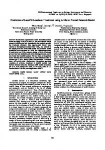
n Artificial Neural Networks Artificial neural networks (ANNs) have been applied to a large number of problems because of their non-linear system modelling capacity. ANNs are designed to mimic the characteristics of biological neurons in the human brain and nervous system. With given sample vectors, ANNs are able to map the relationship between input and output; they “learn” this relationship, and store it in their parameters. The training algorithm adjusts the connection weights (synapses) iteratively, and learning typically occurs through training. When the network is adequately trained, it is able to generalise relevant output for a set of input data. Multi layer perceptron (MLP) A typical MLP network is arranged in layers of neurons, where each neuron in a layer computes the sum of its inputs and passes this sum through an activation function (f). The architecture of an MLP type ANN is presented in Figure 1. To train the MLP with back-propagation, the first step is propagating the inputs towards the forward layers through the network. For a three-layer feed-forward network, the training process is initiated from the input layer [24]: a0 = u am+1 = fm+1(Wm+1am + bm+1), (2) m = 0,1 y = a3 Where y is the output vector, u - the input vector, f(.) - the activation function, W weighting coefficients matrices, b – the
11
steepest descent rule, the error is decreased repeatedly. Elman recurrent neural networks (ERNN) ERNN (also known as partially recurrent neural networks) are a subclass of recurrent networks. It is an MLP network augmented with additional context layers (W0) and storing output values (y), with one of the layers delayed (z-1) by one-step and used for activating the other layer in the next time (t) step [25].
Figure 1. MLP type ANN architecture [23].
y (t +1) = f 1 ( W1x + b1 ) + y (t) W 0 y (t +1) = f 1 ( W1x + b1 ) + y (t) W 0
Figure 2. ERNN type ANN architecture [23].
bias factor vector, and m is the layer index. These matrices are defined as w1,1 w 2,1 W1 = . wS 1,1 2
w1,2 w2,2 . wS 1,2
... w1, S 0 ... . , ... w2, S 0 ... wS 1, S 0
d3 = -2F3(n3)(e) d = Fm(nm)(Wm+1)Tdm+1 for m = 2, 1 m
W = [w1,1 w1,2 ... w1,S1] b1 = [b1 b2 bS1]T, b2 = [b1]
In this study, sigmoid tangent activation functions are used for the hidden layer and the linear activation function for the output layer, respectively. These functions are defined as follows: (exp n − exp − n ) f1 = , f (exp n + exp − n )
2
= n (3)
The total network output is s m −1
nim = ∑ wim, j a mj −1 + bim j =1
(4)
The second step is propagating the sensibility s (d) from the last layer to the first layer through the network: d3, d2, d1. The error (e) calculated for output neurons is propagated backwards through the weighting factors of the network, which
∂f m (n m ) 1 m ∂n1 . m m mm F F (n 0 (n )) = = 0
Equation 6.
12
can be expressed in matrix form as follows:
(5)
Fm(nm) is a Jacobian matrix (Equation 6); e is the mean square error,
e=
1 q g g g 2∧ g 2 ∑ (y( y- y−) y ) (7) 2 g =1
where g is a sample of dimension q. The last step in back-propagation is updating the weighting coefficients. The state of the network always changes in such a way that the output follows the error curve of the network downwards. W m (k + 1) = W m (k ) − α d m (a m −1 )T b m ( k + 1) = b m ( k ) − α d m
(8)
where α represents the training rate and k - the epoch number. Using the algorithmic approach, known as the gradient descent algorithm, and the approximate
0
0
∂f m (n2m ) ∂n2m
0
0
∂f m (nsm3 ∂nsm3
)
(6)
(9)
While ERNNs use an identical training algorithm as MLP, the context layer weight (W0) is not updated as in Equation 6. The architecture of an ERNN type ANN is presented in Figure 2. Selecting the best network architecture The number of hidden layers and neurons therein play a very important role in ANNs, with the choice of these numbers depending on the application. Theoretical works have proved that a single hidden layer is sufficient for ANNs to approximate any complex nonlinear function with any accuracy desired. In addition, how to determine the optimal number of hidden neurons is still a question yet to be answered. Although there is no theoretical basis for selecting these parameters, a few systematic approaches have been reported. However, the most common way of determining the number of hidden neurons is still the trial and error approach. Designed MLPs and ERNNs are trained with backpropagation learning algorithms, as described above. Once trained, the network can be used for predicting the output of any input vector from the input space. This is called the “generalisation property” of the network. To show this property of trained networks, the same experiment is done with a set of test data that is not involved in the set of training data. At the end of the training and testing experiments, the root mean square error (RMSE) values and correlation coefficients (R) obtained are compared. MATLAB with a Neural network toolbox is used for all ANN applications [23]. FIBRES & TEXTILES in Eastern Europe 2011,Vol. 19, No. 3 (86)
n Prediction In this section, prediction efforts realized for MLP and ERNN type ANN architectures and results are given. Then the ARIMA model realised and its result are given. To predict Turkey’s denim trouser export with ANN architectures, 23 input variables were chosen. These input variables, which affect the export of denim trousers, were selected to take into consideration the factors defined in section ‘The study’. The input variables are; 1. Years, (1995–2008), 2. Months, (from the first month of 1995 to the last month of 2008), 3. Turkey’s denim trouser import, 4. Minimum wage in TURKEY, 5. Cotton price on Turkey’s stock-market, 6. Price of electricity for the Turkish industry, 7. Price of water for the Turkish industry, 8. Turkish lira to USD exchange rate, 9. Credit usage of readymade clothing and confection sector, 10. Export credit prior to consignment, 11. Foreign trade enterprise credit, 12. Export credit, 13. Transport costs, 14. Export credit SME, 15. Export credit prior to consignment, (foreign currency), 16. Foreign trade enterprise credit (foreign currency), 17. Export credit (foreign cur-
Table 1. Different MLP Model Training, Testing and Prediction data, RMS Error and Correlation Coefficient (R). Model 1 / 20
Hidden Layer Neuron No.
Training (1995-2006)
Test (1995-2006)
Prediction (20072008)
1.
2.
RMSE
R
RMSE
R
RMSE
R
20
-
6.7685×10⁻³¹
1
0.0444
0.9413
0.0644
0.2724
1 / 30
30
-
1.2880×10⁻²²
1
0.0705
0.8798
0.0676
0.5385
2 / 15 / 20
15
20
1,0661×10-09
1
0.0282
0.9549
0.0477
0.5699
2 / 15 / 40
15
40
2.3802×10⁻²⁵
1
0.0815
0.8438
0.0993
0.6639
2 / 25 / 35
25
35
2.8099×10⁻²⁵
1
0.0618
0.9222
0.0449
0.7472
2 / 30 / 5
30
5
3.3465×10-04
0.999
0.0541
0.9065
0.0294
0.7708
2 / 30 / 20
30
20
4.1093×10⁻²⁵
1
0.0304
0.9593
0.0313
0.7999
2 / 35 / 30
35
30
9.5405×10⁻³¹
1
0.0781
0.8245
0.0493
0.8224
2 / 40 / 5
40
5
1.3636×10-05
1
0.0208
0.8692
0.0165
0.8768
2 / 40 / 25
40
25
8.1273×10⁻³¹
1
0.0754
0.9688
0.0089
0.9314
rency), 18. Pre-consignment rediscount credit – DISCOUNT, 19. Transport shipping marketing credit, 20. Export credit SME (foreign currency), 21. Manufacturer price index based on the real effective exchange rate, 22. Denim trouser brand registration no, 23. Denim trouser Balasa index Prediction with MLP network To find the best MLP model, 10 experiments were realized, the training, testing and prediction results of which are shown in Table 1.
As seen in Table 1, model number 2 / 40 / 25 gives the best result according to RMSE and R values. This model has got two hidden layers. There are 40 neurons in the first hidden layer and 25 neurons in the second. In Figure 3.a, the model’s training data regression tendency is examined, and it can be seen that the R value in the training data set is 1. This value shows the complete realisation of the training. In Figure 3.b, the output graph shows that the full modelling process is supplied.
a)
b)
Figure 3. MLP network 2 / 40 / 25 model’s training data correlation coefficient (a) and training data output (b). a)
b)
Figure 4. MLP network 2 / 40 / 25 model’s test data correlation coefficient (a) and test data output graph (b). FIBRES & TEXTILES in Eastern Europe 2011, Vol. 19, No. 3 (86)
13
a)
b)
Figure 5. MLP network 2 / 40 / 25 model’s prediction data correlation coefficient (a) and prediction data output graph (b).
a)
b)
Figure 6. ERN network 2 / 30 / 30 model’s training data correlation coefficient (a) and training data output graph (b).
a)
b)
Figure 7. ERN network 2 / 30 / 30 model’s test data correlation coefficient (a) and test data output graph (b).
a)
b)
Figure 8. ERN network 2 / 30 / 30 model’s prediction data correlation coefficient (a) and prediction data output graph (b).
14
FIBRES & TEXTILES in Eastern Europe 2011,Vol. 19, No. 3 (86)
In Figure 4.a, the model’s test results are shown. Here, the R value is 0.9688, which shows that the test is not completely successful; however, the test results and input data come close to each other. The situation is seen in more detail in Figure 4.b. In the first couple of months, the ANN output follows real output values, but the gap between them is increasing. In order to examine the forecasting ability of this model, the export values of 2007-2008 were predicted. When the prediction regression graph in Figure 5.a is examined, it is seen that the correlation coefficient has a very good value of 0.931. The predictions for 2007-2008 are shown in more detail in Figure 5.b. As seen in Figure 5.b, the ANN and output values of 2007-2008 are very coherent. When the regression curves in Figure 5.a and the prediction graph of the model are analysed, it can be concluded that this ANN model can be used to predict Turkey’s denim trouser export. Prediction with an Elman recurrent network
Table 2. Different ERNN Model Training, Testing and Prediction data, RMS Error and Correlation Coefficient (R). Model
Hidden Layer Neutron No.
Training (1995-2006)
Test (1995-2006)
Prediction (2007-2008)
1.
2.
RMSE
R
RMSE
R
RMSE
R
1 / 25
25
-
8.2729×10⁻²⁹
1.0000
0.0855
0.8975
0.1480
0.1666
1 / 50
50
-
6.1662×10-05
0.9999
0.0316
0.9440
0.0582
0.5344
2 / 5 / 30
5
30
1.6350×10⁻³
0.9976
0.0393
0.9775
0.0490
0.5924
2 / 10 / 50
10
50
7.3932×10⁻³¹
1.0000
0.0505
0.9261
0.0397
0.6483
2 / 15 / 15
15
15
1.4161×10-04
0.9998
0.0331
0.9541
0.0549
0.7767
2 / 15 / 20
15
20
1.0781×10-05
1.0000
0.0402
0.9420
0.0435
0.7808
2 / 20 / 5
20
5
7.5731×10-04
0.9992
0.0130
0.9698
0.0252
0.7845
2 / 25 /25
25
25
3.0426×10⁻¹²
1.0000
0.0797
0.9274
0.2055
0.7891
1.0000
0.0358
0.9477
0.0184
0.8545
1.0000
0.0237
0.9565
0.0146
0.8938
2 / 25 / 40
25
40
5.5224×10⁻²⁷
2 / 30 / 30
30
30
9.2562×10⁻³¹
Table 3. Estimation of parameters. Term AR 1
Coefficient
Standard Error of Coefficients
T
P
-0.6568
0.0856
-7.67
0.000
AR 2
-0.4807
0.0925
-5.20
0.000
AR 3
-0.2456
0.0846
-2.90
0.004
SAR 12
0.4109
0.0851
4.83
0.000
Constant
0.0216
0.0138
1.57
0.118
To find the best ERNN model, 10 experiments were realised, the training, testing and prediction results of which are shown in Table 2. According to the test results in Table 2, the ERNN model that gives the best results in terms of RMSE and R is model number 2 / 30 / 30, which has got two hidden layers, with 30 neurons in both the first and second hidden layers. In Figure 6.a, the R value in the training process equals 1, showing the complete realisation of the training. A complete modelling was obtained during the training process, as can be clearly seen in Figure 6.b. The R value in the testing process is 0.956, as shown in Figure 7.a, demonstrating that although the testing is not completely realised, it has a very little error. In Figure 7.b. The testing Graph of the Model is given. The ANN values are compatible with the output ones. In order to examine the forecasting ability of this model, the export values of 2007-2008 were predicted. When the regression graph in Figure 8.a is analysed, it is seen that the correlation coefficient is 0.893. The predictions outputs for 20072008 are given in Figure 8.b. The ANN FIBRES & TEXTILES in Eastern Europe 2011, Vol. 19, No. 3 (86)
Figure 9. Prediction of Turkey’s denim trouser export per month using the ARIMA model.
and output values of 2007-2008 are very consistent with each other. Hence it can be concluded that this ANN model can be used to predict Turkey’s denim trouser export. After completing MLP and ERN Network testing to predict Turkey’s total denim trouser export, it can be seen that the MLP Network has a better prediction performance than the ERNN architecture. Prediction with an ARIMA model In order to fit an ARIMA model to denim trouser export data, an attempt was made to stabilise both the variance and mean of
the data. In order to stabilise the variance, the data was transformed by using a logarithm with base e. After taking the logarithm, the difference was first obtained to stabilise the mean of the data. To create an appropriate ARIMA model, (3, 1, 0) (1, 0, 0)12 was fitted to the data. The ARIMA (3,1,0)(1,0,0)12 model used for prediction is; Yt = c + f1Yt-1 + (f2 - f1)Yt-2 + + (f3 - f2)Yt-3 - f3Yt-4 + F1Yt-12 + (9) - (f1F1 + F1)Yt-13 - (f2F1 - f1F1)Yt-14 + - (f3F1 - f2F1)Yt-15 - f3F1Yt-16 + et where Y = Lny
15
Figure 10. Comparative graph of the prediction of Turkey’s denim trouser export for the years 2007-2008 using different models.
The parameter estimates from Table 3 are put in place as f1 = -0.6568, f2 = -0.4807, f3 = -0.2456, F1 = 0.4109 and c = 0.02161. The prediction graph seen in Figure 9 (see page 15) was created by transforming the Lny values predicted back into real values by eY.
n Conclusion The prediction of Turkey’s denim trouser export in 2007-2008 was realised using ANN and ARIMA models. The predictions can be seen in Figure 10. When they are analysed, it is seen that generally ANN and ARIMA models cannot completely model denim trouser export. It is observed that the best prediction is provided by MLP, the second with ERNN and the third with ARIMA. The reason why denim trouser export cannot be completely modelled may be explained by the economic downturn, which began in 2008 and still continues. However, it is clearly seen that ANNs predict more successfully than an ARIMA model. After completing the study, it could be concluded that denim trouser export can be foreseen using ANNs. If all the factors that influence export are added to the model, better predictions can be obtained with ANNs. However, it is not possible to include all factors in the model. For instance, economic downturns are very hard to anticipate and to model. Moreover most of the socio-economic factors can directly or indirectly influence export but are not included in the model because they are very difficult to transform into quantitative variables. When all these restrictions are considered, our study
16
shows that ANNs provide better predictions of denim trouser export.
References 1. Koutroumanidis T.; Ioannou K.; Arabatzis G. “Predicting Fuelwood Prices in Greece with the Use of ARIMA Models, Artificial Neural Networks and Hybrid ARIMAANN Model” Energy Policy 37, 2009, pp. 3627-3634. 2. Geem Z. W.; Roper W.E. “Energy Demand Estimation of South Korea using artificial Neural Network” Energy Policy, 37, 2009, pp. 4049-4054. 3. Karaali F. Ç. Ulengin F.; “Predicting Unemployment Rates With The Use Of Cognitive Mapping Methodology And Artificial Neural Networks” İtüdegisi/d Engineering Vol.7, Num.3, 2008, pp. 15-26. 4. Co C., H.; Boosarawongse R. (2007) “Forecasting Thailand’s Rice Export: Statistical Techniques vs. Artificial Neural Networks” Computers & Industrial Engineering 53, Page. 610-627. 5. Usta A.S.: “Forecasting Model And Analyse Of Producers Price İndex (PPI) İn Turkey By Using Artificial Neural Network Application” MSc. Thesis, Yıldız Technical University, 2007, Turkey. 6. Zou H.F.; Xia G.P.; Yang F.T.; Wang H.Y.: “An Investigation and Comparison of Artificial Neural Network and Time Series Models for Chinese Food Grain Price Forecasting” Neurocomputing 70, 2007, pp. 2913-2923. 7. Ertuğrul I.; Tokat S.; Aytac E.; Tus A. “A Case Study For Forecasting Denizli City Manufacturing Industry Export Data Using Artifıcial Neural Networks” Proceedings of 4th International Symposium on Intelligent Manufacturing Systems, Sakarya University, Turkey, 2005. 8. Bas N. “Artificial Neural Networks Approach And An Application” MSc. Thesis, Mimar Sinan Arts University, Turkey, 2006. 9. Bayır F. “Artificial Neural Networks And Application On Forecasting” MSc. Thesis, Istanbul Technical University, Turkey, 2006.
10. Glenn A. R.; “Finished Good Sourcing Decisions in The US Apparel Industry After Implementation Of The Agrement on Textiles and Clothing” Degree Doctor of Philosophy, The Ohio State University, USA, 2006. 11. Kabal A.K. “The Economic Policies Practised İn Between 1980-2005 And Their Effects On Foreign Trade” MSc. Thesis, Ataturk University, Turkey, 2007. 12. Ongüt, Ç. E. “Türk Tekstil ve Hazır Giyim Sanayinin Değişen Dünya Rekabet Şartlarına Uyumu” Speciallization Thesis, T.R. Prime Ministry State Planning Organization, Turkey, 2007. 13. Keleş İ.; “The Characteristics Of Textile And Clothes Sectors And The Position And İmportance Of Them İn Turkish Export” MSc. Thesis, Gazi University, Turkey, 2000. 14. Colak G. “Export Incentives and Türk Eximbank” MSc. Thesis, Gazi University, Turkey, 2007. 15. Varoçlu Ö. “Turk Eximbank And The Role Of Suppoting Export” MSc. Thesis, Kocaeli University, Turkey, 2005. 16. Topcul M. “Türk Eximbank Kredi Programları, İhracat Kredi Sigortası ve Garantisi” MSc. Thesis, Marmara University, Turkey, 2004. 17. Çifci S. “Brand And Brand Loyalty: An İnvestigation About University Students’jean Choices And Brand Loyalty” MSc. Thesis, Abant İzzet Baysal University, Turkey, 2006. 18. Görgülü A. “Branding İn Textile And Apparel İndustry İn Turkey And İts İnfluence On Export” MSc. Thesis, Uludağ University, Turkey, 2006. 19. Çıplak U. “Competitiveness İndicators And An Evaluation With Respect To Turkish Manufacturing İndustry Goods Exports” MSc. Thesis, Gazi University, Turkey, 2007. 20. Zengin A. “Reel Döviz Kuru Hareketleri ve Dış Ticaret Fiyatları (Türkiye Ekonomisi Üzerine Ampirik Bulgular)” C.Ü. İktisadi ve İdari Bilimler Dergisi, Vol. 2, Number 2, 2000. 21. Kök R., Çoban O.; “The Turkish Textile Industry and its Competitiveness: A Comparative Analysis with the EU Countries during the period 1989-2001” İktisat İşletme ve Finans, Vol. 20, Issue: 228, 2005, pp. 68-81. 22. Aynagöz Ç. Ö. “Açıklanmış Karşılaştırmalı Üstünlükler ve Rekabet Gücü: Türkiye Tekstil ve Hazır Giyim Endüstrisi Üzerine Bir Uygulama” Ege Academic Review, Vol. 5, Number 1-2, 2005. 23. Demuth H.; Mark B.; “ Neural Network Toolbox User’s Guide” The MathWorks, Inc. MA, 2002. 24. Hagan T. M; Demuth H.B; Beale M.; “Neural Network Design” PWS Publishing Company, 1996, pp. 2-44. 25. Elman J. L.; “Finding Structure in Time” Cognitive Science, 14, 1990, pp. 179-221. Received 21.06.2010
Reviewed 21.07.2010
FIBRES & TEXTILES in Eastern Europe 2011,Vol. 19, No. 3 (86)