Hindawi Publishing Corporation International Journal of Atmospheric Sciences Volume 2014, Article ID 141923, 12 pages http://dx.doi.org/10.1155/2014/141923
Research Article Predictive Ability of Improved Neural Network Models to Simulate Pollutant Dispersion Khandaker M. A. Hossain Department of Civil Engineering, Ryerson University, 350 Victoria Street, Toronto, ON, Canada M5B 2K3 Correspondence should be addressed to Khandaker M. A. Hossain;
[email protected] Received 28 February 2014; Accepted 7 May 2014; Published 26 June 2014 Academic Editor: Prodromos Zanis Copyright © 2014 Khandaker M. A. Hossain. This is an open access article distributed under the Creative Commons Attribution License, which permits unrestricted use, distribution, and reproduction in any medium, provided the original work is properly cited. This paper describes the ability of artificial neural network (ANN) models to simulate the pollutant dispersion characteristics in varying urban atmospheres at different regions. ANN models are developed based on twelve meteorological (including rainfall/precipitation) and six traffic parameters/variables that have significant influence on emission/pollutant dispersion. The models are trained to predict concentration of carbon monoxide and particulate matters in urban atmospheres using field meteorological and traffic data. Training, validation, and testing of ANN models are conducted using data from the Dhaka city of Bangladesh. The models are used to simulate concentration of pollutants as well as the effect of rainfall on emission dispersion throughout the year and inversion condition during the night. The predicting ability and robustness of the models are then determined by using data of the coastal cities of Chittagong and Dhaka. ANN models based on both meteorological and traffic variables exhibit the best performance and are capable of resolving patterns of pollutant dispersion to the atmosphere for different cities.
1. Introduction Air pollution is a major environmental concern in major cities around the world. The major causes of air pollution include rapid industrialization and urbanization and increased non-environment-friendly energy production. The emission of pollutants such as carbon monoxide (CO), nitrogen oxides (NOx/NO2 ), and particulate matter (PM) due to high traffic volumes, congestion, and poor vehicle maintenance has resulted in the transport sector being a major contributor to air pollution in major cities around the world [1]. Inefficient land use and overall poor traffic management further add to traffic congestion and air pollution besides old, overloaded, and poorly maintained motor vehicles [2, 3]. Although the concentration of particulate matter with an aerodynamic diameter of less than 10 𝜇m (PM10) is usually used as standard measure of air pollution, the particles with a diameter of less than 2.5 𝜇m (PM2.5) have been associated with the increase of health related problems [4]. Air quality data are complex and nonlinear in nature because of their dependencies on emission sources, especially
those related to vehicular emissions and meteorological parameters. One approach to predict pollutant concentrations is to use a detailed atmospheric diffusion model that requires detailed emissions and metrological data [5]. Another approach is the regression modeling based on a statistical approach that has been applied to air quality modeling and prediction. However, such linear regression models underperform when used to model nonlinear systems [6]. Artificial neural network (ANN) is capable of capturing highly nonlinear phenomena and can be used as a tool for the development of models to predict atmospheric emissions. The ANN approach has been used with some success to model pollutant concentrations in previous studies [7–12]. The approach has also been applied to various civil engineering problems, such as structural damage detection [13], material behavior modeling [14], and structural optimization [15]. Vehicular exhaust emission dispersion characteristics in cities near roadways were studied using ANN based line source models (LSMs) [9, 16]. Unlike traditional parametric models, an ANN does not have to assume a model form between the input and output variables. The ANN consists of multiple
2 layers of many interconnected linear or nonlinear processing units operating in a parallel fashion. The nonlinear nature of neural networks makes them suitable to perform functional approximation, classification, and pattern recognition [17]. Previous research studies based on ANN modeling concentrate on the prediction of NOx/NO2 and CO concentrations or dispersion characteristics in urban atmosphere taking into account meteorological (excluding the effect of rainfall) and vehicular parameters [6, 8–10]. However, Melas et al. [12] considered the rainfall as an input in ANN modelling of NO2 . A limited study has been conducted to predict PM2.5 concentration using ANN modeling considering only three meteorological parameters (temperature, wind velocity, and relative humidity) [8, 11]. ANN modeling has not been applied to model particulate matter (both PM10 and PM2.5) dispersion in an urban atmosphere combining both vehicular and meteorological parameters. This paper presents the performance of refined ANN models for the prediction of concentrations of carbon monoxide and particulate matters (PM10 and PM2.5) in the atmosphere in an urban setup (Dhaka city, Bangladesh) considering both vehicular emissions and meteorological parameters (including precipitation/rainfall as an additional parameter which was not included in previous research studies). The refined models are updated versions of preliminary models [18] and are trained with large volume of data for enhanced performance in wide range of urban atmospheres. The predictive ability and robustness of the models are tested with data from the coastal city of Chittagong and different locations of Dhaka. Although preliminary ANN models are applied for pollutant dispersion in Dhaka city, there is an urgent need to do research in refining the models and to predict their ability to simulate pollutant dispersion in different cities in Bangladesh. The proposed refined and robust ANN models can be very useful for various government agencies and other organizations involved in the air quality management of urban areas.
2. Development of Artificial Neural Network Models The basic methodology for developing a successful ANN based model is to teach a neural network the relationship between inputs and outputs using existing data. In this study, various combinations of meteorological, vehicular, and traffic parameters are used as inputs in the feed forward-back propagation ANN to obtain as outputs the concentration of CO and particulate matter (PM10 and PM2.5) in the atmosphere. Besides data collection, three important steps are considered in constructing a successful artificial neural network: network architecture, training, and testing. In this study, the most commonly used “back-propagation network” [17] is implemented. 2.1. Data Collection and Description (from Dhaka and Chittagong). The degree of success of the ANN model prediction depends on the comprehensive training data, capable of teaching the network all aspects of the relationship between
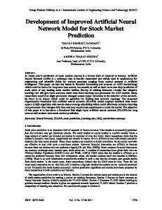
International Journal of Atmospheric Sciences inputs and outputs. Monitoring of ambient air quality in Bangladesh is initiated in 1990 on a very limited basis by the Department of Environment (DOE) using high-volume samplers [2, 19]. The acuteness of the problem caused by air pollution has made the government aware of the necessity to monitor ambient air quality in 2002. Continuous air quality monitoring station (CAQMS) was established by DOE at the parliament building in the centre of the Dhaka city. There are also a number of other organizations (such as Bangladesh University of Engineering & Technology and Bangladesh Atomic Energy Centre) that monitor Dhaka’s air quality as well as emissions from the automobiles. This study is based on the data collected from Dhaka (capital of Bangladesh) and port city of Chittagong situated at the shoreline of Bay of Bengal, 250 km south of Dhaka. Hourly CO, PM10, and PM2.5 concentration data (collected between January 2004 and December 2004) form the basis of this study. Meteorological data such as temperature, wind speed, wind direction, precipitation (rainfall), cloud cover, pressure, mixing height, sunshine, visibility, and humidity are collected from the Bangladesh Meteorological Department and consulted from other sources. The typical variation of some meteorological parameters compiled from the data of Dhaka city over a year period (during 2004) is presented in Table 1. In Chittagong, wind blows from north-east direction (from land to sea) in the winter season and from the southeast direction (sea to land) during the summer (monsoon) season. During the duration of this study, the wind speed ranged from 2.9 to 5.8 m/s, the temperature ranged from 27 to 32∘ C, the humidity ranged from 78 to 88%, and the total rainfall was around 2100 mm (with monsoon season having heavier rainfall like Dhaka). The values of these meteorological parameters differed in different seasons between Dhaka and Chittagong over the year. In Dhaka, the data was collected independently by the research team (between January and December of 2004) from an air quality monitoring (AQM) station located close to CAQMS [20]. The data obtained from the CAQMS and other sources are also consulted. The data on hourly traffic volume at the site (line source) were monitored during the study period (between January and December 2004) by the author’s research team. Limited available data from other local sources were also consulted. Figure 1 shows the locations of AQM station and the site (line source) for the traffic data (near the AQM station) situated at one of the busiest intersections in Dhaka [20]. In Chittagong, air quality monitoring station (AQM) and line source were situated near the busiest intersection at Agrabad commercial area. The sites (line source) for the traffic data in both Dhaka and Chittagong cites were located within 200 m of the AQM station. The results of the air quality monitoring in Dhaka and Chittagong show that particulate matter (PM10 < 10 𝜇m and PM2.5 < 2.5 𝜇m) is one of the pollutants of major concern besides other emissions such as CO, NOx, SO2 , and Ozone (O3 ) [3, 19–21]. Based on local traffic types and compositions of Dhaka and Chittagong cities, vehicles were classified as follows: twowheeler (motor cycle), three-wheeler (auto-rickshaw, autotempo, and baby taxi), and four-wheeler gasoline-powered
International Journal of Atmospheric Sciences
3
Table 1: Average meteorological parameters in Dhaka during 2004. Average values Season Winter Premonsoon Monsoon Postmonsoon
∘
Temp. ( C) Rainfall Relative humidity Wind speed Prevailing wind direction Max. Min. (mm) (%) (m/s) 28 35 30 30
12 22 27 21
65 515 1198 225
70 72 82 77
0.9 1.7 1.5 0.7
% calm 2 m/s) 9 42 36 8
Winter: Dec.–Feb.; premonsoon: March–May; monsoon: June–Sept.; postmonsoon: Oct.-Nov.
Figure 1: Dhaka city map showing air quality monitoring station and line source.
vehicles; four-wheeler (e.g., car, truck, bus, minibus, and wagon) diesel-powered vehicles. The emission factors used for estimating the CO and PM10 source strengths are presented in Table 2 [22]. The main pollutants of concern in Dhaka are the particulate matter (PM) and motor vehicles are the major contributors to PM pollution. Most of the vehicular PM pollution (>80%) comes from the diesel vehicles as can be seen from Table 2. This is also the situation for NOx and SO2. However, nondiesel vehicles are the major sources of CO in the air (about 82%). The trend over the year shows an increase in the PM concentration (𝜇g/m3 ) from October to April, beyond which the concentration of both PM10 and PM2.5 decreases due to the rain-out effect. From November to March, both PM concentrations exceed the proposed standards of 150 𝜇g/m3 for
PM10 and 65 𝜇g/m3 for PM2.5, the latter being far in excess of the proposed standards. A similar trend of variation is also found for CO over the year. PM and CO concentration drops in the premonsoon and monsoon seasons (between May and September) due to rainfall or precipitation [20]. The field data also shows the development of inversion condition where the concentration of pollutants increases at night even with the significant decrease in traffic volume. It is also observed that the rainfall during the day and at night can significantly affect the inversion condition. Therefore, consideration of rainfall besides other meteorological parameters in an ANN model is important for tropical countries like Bangladesh to model emission dispersion characteristics throughout the year. The amount of turbulence in the ambient atmosphere has a major effect on the dispersion of air pollution plumes because turbulence increases the entrainment and mixing of
4
International Journal of Atmospheric Sciences Table 2: Vehicular data in Dhaka in 2004. Vehicle emission
Emission categories
% of total emission CO PM10
Emission factors Emission factors gram/km Emission categories CO PM10
Cars
66.5
7.9
Gasoline vehicle
25
0.1
Taxis-CNG
2.8
0.5
CNG taxis
5
0.03
3-wheel taxis-CNG
3.8
0.7
LD diesel Buses Trucks
3.9 8.2 5.9
Motorcycles Total
Number of vehicles on the road Vehicle type
Number
Motor car Jeep/station wagon /microbus
81703 30581
5
0.03
Taxi
4389
18.6 38.9 28.1
CNG auto-rickshaws Diesel vehicles Buses Trucks
5 10 10
0.80 1.60 1.60
2140 6409 18214
8.9
5.3
Motorcycles
5
0.10
Bus Minibus Truck Autorickshaw/tempo
100
100
Motor cycle
29120 112060
Emission (%): diesel and nondiesel vehicles Diesel
18
82.4
Nondiesel
82
17.6
Total CO emissions from vehicles in 2004 = 71,793 tons Total PM10 emissions from vehicles in 2004 = 2412 tons
Temperature Wind speed Wind direction (sin) Wind direction (cos) Cloud cover 12 Pressure meteorological Pasquill stability (M) variables Mixing height Sunshine hour Visibility Rainfall Humidity Two-wheeler Three-wheeler 6 Four-wheeler gasoline traffic (T) Four-wheeler diesel variables Source strength of CO Source strength of PM10 Input layer
Output CO/PM10/ PM2.5
Hidden layer
Output layer
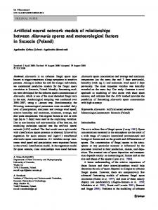
Figure 2: Architecture of typical ANN based MT model (18 : 4 : 1).
unpolluted air into the plume and thereby acts to reduce the concentration of pollutants in the plume. It is therefore important to categorize the amount of atmospheric turbulence present at any given time. In this study, the PasquillGifford stability scheme is used to determine hourly stability categories as used by other researchers [23, 24]. The ANN models take into account any discontinuities in the original cyclic signals of wind direction data by using the sine and cosine functions [6, 9]. 2.2. Network Architecture Optimization. The first fundamental step in constructing a neural network model is to determine the network architecture. The basic aspects of
network architecture (as shown in Figure 2) consist of the number of hidden layers between the input and output layers, the number of processing units in each layer, the pattern of connectivity among the processing units, and the activation (transfer) function employed for each processing unit [17]. For a given architecture, it is the weights between the processing units that determine the network performance. Figure 2 shows information on the meteorological (M) and traffic (T) input data and a typical ANN architecture used for developing various ANN models to predict the 1 h average CO, PM10, and PM2.5 concentrations. Twelve “M” input variables are temperature, wind speed, wind direction (sin), wind direction (cos), cloud cover, pressure, Pasquill
International Journal of Atmospheric Sciences stability, mixing height, sunshine hour, visibility, rainfall, and humidity. Six “T” input variables are hourly volumes of twowheeler, three-wheeler, and four-wheeler gasoline-powered vehicles; four-wheeler diesel-powered vehicles; and source strength of CO and source strength of PM10. Three types of ANN models are developed (using the data from Dhaka city) to study the individual and the combined effect of meteorological and vehicular parameters on CO, PM10, and PM2.5 dispersion characteristics. These models are based on preliminary ANN models [18] and use comparatively large number of data in training, validation, and testing compared to their primary counterparts. Hence, these models are more efficient and accurate than preliminary models in varying urban atmospheres. The first model considers both meteorological and traffic characteristics data (designated as ANN-MT in Figure 2), the second model considers only meteorological data (designated as ANN-M), and the third model considers only traffic data (designated as ANN-T). Data sets used for training, validation, and testing of each of the nine ANN models are as follows: (i) those predicting CO (ANN-MT-CO, ANN-M-CO, and ANN-T-CO) are 4995, 1912, and 1713, respectively; (ii) those predicting PM10 (ANNMT-PM10, ANN-M-PM10, and ANN-T-PM10) are 4361, 1876, and 1717, respectively; and (iii) those predicting PM2.5 (ANN-MT-PM2.5, ANN-M-PM2.5, and ANN-T-PM2.5) are 4319, 1574, and 1312, respectively. Training data set (from Dhaka city) covers the complete period of study from January 2004 to December 2004. The testing data set chronologically follows the period that is used for validation. There were no qualitative differences between the training and the testing data set. The flow of traffic was measured to obtain hourly variations and traffic input parameters in the ANN models reflect the variation with time. 2.3. Training of ANN Models. ANN models are trained by using back-propagation technique with momentum term algorithm. Training a back-propagation neural network is an iterative process; involving the presentation of field data as pairs (input/target) and having the network modify its weights by the invocation of learning rules until it stabilizes [17]. Each training pair consists of an input vector containing meteorological or traffic variables or both and a target representing the concentration of emissions. The network is presented with the data in the first input vector, carries out the appropriate computation and activation through the processing units in the hidden layers, and then produces an output through the unit in the output layer. The network compares its output to the corresponding target which is provided in the training pair. The difference between the network output and the target is calculated and stored. After this procedure is done with the first training pair, called the training pattern, the network is presented with a second training pair and so on until the network has gone through all the data available for training; that completes the first epoch. After each epoch, the network calculates the mean square of all errors it calculated and stored after each training pattern and back-propagates it using the network learning algorithm to adjust the weights
5 and biases for all units in the network. The training continues until either the network converges and reaches its goal for the minimum error between the predicted values and the desired target provided for training or the maximum number of epochs specified for early stopping is reached. In the current study, the degree of agreement (𝜉) and the root mean square error (RMSE) values are estimated to evaluate the performance of the trained models as used in previous research studies [25]. The value of 𝜉 is calculated as [25] 2
∑𝑛𝑗=1 (𝑃𝑗 − 𝐹𝑗 ) 𝜉=1− 2, ∑𝑛𝑗=1 [𝑃𝑗 − 𝐹mean − 𝐹𝑗 − 𝐹mean ]
(1)
where 𝑛 is the number of data points, 𝐹𝑗 are the field observation data points, 𝑃𝑗 are the predicted data points, and 𝐹mean is the mean of the observed data points. A value of 1 indicates perfect agreement between the observed and predicted values while 0 denotes complete disagreement. Extensive simulations were performed to determine the best combination of parameters involving network architecture, mathematical function, and solution algorithm such as learning rate (𝜂), momentum constant (𝜆), number of hidden layers, number of hidden neurons, learning algorithm, and activation function. An 18 : 4 : 1 feed-forward neural network (with 18 neurons in the input layer, 4 neurons in the single hidden layer, and 1 neuron in the output layer) provided the best prediction for the validation data set with both meteorological and traffic (MT) variables. The architecture of such 18 : 4 : 1 ANN-MT model with total 18 meteorological and traffic input variables is presented in Figure 2. The 12 : 4 : 1 ANN-M models are developed with 12 meteorological variables (with 4 neurons in single hidden layer), while the 6 : 4 : 1 ANN-T models are developed with 6 traffic variables (such as two-wheeler, three-wheeler, four-wheeler gasolinepowered vehicles, four-wheeler diesel-powered vehicles, and source strength of CO and source strength of PM10) with four neurons in single hidden layer (Figure 2). The architectures of the developed ANN models are different compared to those of previous research studies [7, 9] because of the differences in the combination of various parameters and inclusion of new parameters such as rainfall and particulate source strength factor. The developed ANN models are also able to take into account the effect of rainfall which is a very important meteorological parameter affecting the emission dispersion particularly in tropical countries (due to washout effect) like Bangladesh. Table 3 presents a summary of the ANN model parameters and their performance statistics for the validation data set.
3. Performance Evaluation Statistical factors such as RMSE, mean bias error (MBE), mean square error (MSE), coefficient of determination (𝑟2 ), and mean of the field (𝐹mean ) and predicted (𝑃mean ) values with their standard deviations (𝜎𝑜 and 𝜎𝑃 ) are used to evaluate the performance. Table 4 shows the performance statistics of the ANN models for CO, PM10, and PM2.5 predictions,
6
International Journal of Atmospheric Sciences Table 3: Performance statistics of ANN models on the validation data set (Dhaka).
Model ANN-MT-CO (18 : 4 : 1) ANN-M-CO (12 : 4 : 1) ANN-T-CO (6 : 4 : 1) ANN-MT-PM10 (18 : 4 : 1) ANN-M-PM10 (12 : 4 : 1) ANN-T-PM10 (6 : 4 : 1) ANN-MT-PM2.5 (18 : 4 : 1) ANN-M-PM2.5 (12 : 4 : 1) ANN-T-PM2.5 (6 : 4 : 1)
𝜂 0.001 0.001 0.001 0.001 0.001 0.001 0.001 0.001 0.001
Number of epochs 1800 1300 300 1700 1400 300 1600 1300 300
𝜆 0.6 0.4 0.7 0.7 0.3 0.6 0.6 0.4 0.6
𝜉 0.69 0.63 0.40 0.73 0.54 0.39 0.67 0.51 0.40
RMSE 1.89 2.18 3.39 2.08 2.41 3.09 2.46 2.41 2.89
Table 4: Performance of ANN models for prediction of CO, PM10, and PM2.5 (Dhaka). Model ANN-MT-CO ANN-M-CO ANN-T-CO ANN-MT-PM10 ANN-M-PM10 ANN-T-PM10 ANN-MT-PM2.5 ANN-M-PM2.5 ANN-T-PM2.5
𝐹mean 4.8 4.8 4.8 132.5 132.5 132.5 97.6 97.6 97.6
𝑃mean 5.37 6.89 8.37 154.2 243.1 283.2 118.1 191.2 219.4
𝜎𝑜 2.03 2.03 2.03 5.18 5.18 5.18 4.79 4.79 4.79
𝜎𝑃 1.95 1.79 0.81 4.97 4.52 2.10 4.53 4.12 1.89
MBE 0.73 1.59 3.16 1.79 3.84 7.79 1.65 3.48 7.11
MSE 6.9 8.8 18.1 18.65 23.10 46.11 16.98 21.24 42.10
RMSE 1.98 2.81 5.07 5.52 7.47 13.71 5.07 6.69 12.43
𝑟2 0.47 0.38 0.09 0.43 0.33 0.07 0.33 0.29 0.05
𝜉 0.77 0.62 0.37 0.73 0.54 0.31 0.69 0.51 0.29
F: field concentration; P: predicted concentration; CO concentration in ppm; PM10/PM2.5 concentration in 𝜇g/m3 .
respectively. Based on the goodness of fit PM10/PM2.5 models show poor performance compared with CO model. The mean predicted CO concentration is higher than that of the observed prediction in all three models. The tendency of the models to overpredict is indicated by the positive values of MBE. The tendency of overprediction is less in the MT model followed by the M and T models. This shows that the predictive ability of the MT model is better than that of the other two models. A lower RMSE value for the MT model indicates that the model predictions are matching closely the actual observations. In this regard, the T model shows the worst prediction, while the MT model is the best. The difference between the standard deviation of the field data and the predicted data is high in the T model compared with the M model with the MT model showing the least difference. This explains the fact that the MT model can simulate the variations in the test data whereas M and T models are unable to simulate these variations. The 𝜉 values indicate that the MT model is better in terms of error free prediction compared with the M and T models with the T model being the worst. The MT model produces 77%, 73%, and 69% error free predictions for CO, PM10, and PM2.5, respectively (Table 4). The better performance of MT model can be attributed to the fact that the use of a large number of input variables better represents the nonlinear dispersion dynamics of pollutants and enhances the accuracy of prediction. The distance of the air quality monitoring station from the line source (traffic monitoring site) also affects prediction performance. This
study can be considered as “far-field” as the distance between the traffic monitoring site and the air quality monitoring station is greater than 30 m [26]. In this study, the exclusion of traffic parameters (in the M model) produces better prediction of CO, PM10, and PM2.5 values compared with the model where meteorological parameters are excluded (in the T model). This is attributed to the fact that the meteorological factors mainly disperse and dilute the pollutants in the case of “far-field” and the effect of traffic wake is minimal [27]. Hence, the developed ANN based model is capable of simulating the effects of traffic wake on the dispersion of vehicular emissions. This is also confirmed from previous research studies [9]. In general, the ANN-T models perform poorly in predicting the values of CO, PM10, and PM2.5 (𝜉 ranges from 0.29 to 0.37) because of considering only the traffic variables which takes care of only traffic wake effect. From Table 4, it can be noted that, for all ANN models, the accuracy of prediction is higher for CO (𝜉 ranges from 0.37 to 0.77), followed by PM10 (𝜉 ranges from 0.31 to 0.73) and PM2.5 (𝜉 ranges from 0.29 to 0.69). This can be due to the fact that (a) the variability of PM concentration with respect to vehicular and metrological parameters is higher compared with that of CO and (b) the emission of CO from vehicular source is higher compared with those of PM. 3.1. Performance in Predicting Hourly Pollutant Concentration during a Day. Figures 3 and 4 show the performance of various ANN models in predicting hourly concentration of CO and PM10, respectively, during a day in December in the
35 30 25 20 15 10 5 0
7
CO (ppm)
CO (ppm)
International Journal of Atmospheric Sciences
0
2
4
6
8
10
12
14
16
18
20
22
3.5 3.0 2.5 2.0 1.5 1.0 0.5 0.0
0
2
4
6
Hours of the day Field ANN-MT
ANN-M ANN-T
2
4
6
8
10
12
14
16
18
20
22
PM10 (𝜇g/m3 )
Hours of the day Field ANN-MT
12
14
16
18
20
22
ANN-M ANN-T
Figure 4: Hourly PM10 prediction by various models during the day (Dhaka, AQM station).
winter season. The observed concentrations rise along the day until they reach a peak in the evening hours which implies that clean air is reaching the monitoring site overnight. Pollutant dispersions are mostly influenced by factors such as net wind speed and direction, the variability of wind speed and direction and inversion layers. The air temperature normally reduces with the increase of height and the earth’s surface is the warmest. Normally, the lighter warm air at the earth surface with pollutants slowly rises, a phenomenon that helps in the dispersion of pollutants. However, if a stable layer of colder air sits above warmer air, it forms a blocking or inversion layer that prevents the rise and dispersion of the warm air and the pollutants. This is likely to occur in low or no wind conditions—which is prevalent mostly in winter season in Dhaka city. Figures 3 and 4 also suggest that local sources are responsible for the morning peak of pollution, but later in the day the site becomes a “receptor” of Dhaka’s pollution plume. The field data confirm the inversion effect showing an increase in pollutant concentrations (both CO and PM10) during the night even though the traffic volume decreases significantly. The MT model showed better prediction compared with the M and T models, with the T model being the worst as described earlier. The predictive ability of ANN models depends on how well the local vehicle counts provide a good simulation of the citywide emissions later in the day as well as how well the different processes leading to pollution
ANN-M ANN-T
Figure 5: Effect of rainfall on hourly CO prediction by various models in Dhaka (AQM station).
PM10 (𝜇g/m3 )
0
10
Field ANN-MT
Figure 3: Hourly CO prediction by various models during the day (Dhaka, AQM station). 600 500 400 300 200 100 0
8
Hours of the day
180 160 140 120 100 80 60 40 20 0
0
2
4
6
8
10
12
14
16
18
20
22
Hours of the day Field ANN-MT
ANN-M ANN-T
Figure 6: Effect of rainfall on hourly PM10 prediction by various models in Dhaka (AQM station).
dispersion (involving the impacts of local dispersion in the morning and transport of plumes in the afternoon/evening hours) are simulated. The models are generally trained by assuming that the underlying process is fitted in a single nonlinear process. This simplistic approach for a complex problem is reflected in the worst statistical performance of the models that include traffic or meteorological inputs. The T models also failed to simulate the inversion effect as it does not consider the meteorological parameters as observed in previous research studies [9]. The inversion conditions lead to the trapping of pollutants in the air causing a sharp increase in their concentrations even though the traffic volume decreases to a minimum. In Dhaka, inversion condition normally prevails for 4 to 6 hours after dusk especially during winter season (November to February). The developed MT models seem to simulate the effect of inversion condition on CO, PM10, and PM2.5 reasonably well. Figures 5, 6, and 7 show the performance of various ANN models in predicting hourly concentration of CO, PM10, and PM2.5, respectively, during a rainy day in July in the monsoon season when the effect of rainfall significantly affects the pollutant dispersion in the atmosphere in Dhaka city. The field data confirm the reduction of pollutant concentration during and after the raining periods (rainfall durations: 12 to 16 hours and 20 to 21 hours). The field data also show the effect of rainfall on inversion phenomena. The
International Journal of Atmospheric Sciences 100 90 80 70 60 50 40 30 20 10 0
300
0
2
4
6
8
10
12
14
16
18
20
22
200 150 100 50 1
2
3
ANN-M ANN-T
Field ANN-MT
Figure 7: Effect of rainfall on hourly PM2.5 prediction by various models in Dhaka (AQM station).
MT-PM10 Field-PM10
5 6 8 9 10 4 7 Month (January to December)
11
12
MT-PM2.5 Field-PM2.5
Figure 9: PM10 and PM2.5 prediction by MT model throughout the year in Dhaka (AQM station).
35 30 CO (ppm)
Monsoon: April to September
250
0
Hours of the day
Monsoon: April to September
25 20 15 10 5 0
PM10, PM2.5 (𝜇g/m3 )
PM2.5 (𝜇g/m3 )
8
1
2
3
4
5
6
7
8
9
10
11
12
Month (January to December) MT Field
Figure 8: CO prediction by MT model throughout the year in Dhaka (AQM station).
rainfall before and during inversion period at night reduces the pollutant concentrations and field data do not exhibit any inversion phenomena. The MT model showed better prediction compared with the M and T models, with the T model being the worst. The developed MT models are able to simulate reasonably well the effect of rainfall on pollutant (CO, PM10, and PM2.5) concentrations during and after the rainfall as well as during the inversion period. Figures 5–7 show good agreement between the field data and those predicted by the ANN-MT model based on the duration of a single day taking into account the effect of rainfall/inversion conditions on pollutant dispersions. Such predictive ability of ANN-MT model is valid over the whole year. 3.2. Predicting Ability of Pollutant Concentration at Different Locations of Dhaka City. Figures 8 and 9 show the performance of the best ANN model “MT” in predicting concentration of CO, PM10, and PM2.5, respectively, during a whole year period including monsoon season (April to September). The MT model showed good prediction of all three pollutants compared with field data. This demonstrates that the MT model is able to take into consideration the effect of various meteorological parameters associated with different seasons
(of a year) and, in particular, washout effect (predominant in monsoon season—April to September) due to rainfall that causes a significant decrease in pollutant (CO, PM10, and PM2.5) concentration. The predictive ability of MT model is also illustrated through simulation of CO/PM10/PM2.5 concentrations during a year by using data from CAQMS as shown in Figure 10. It can be noted that the MT models are able to simulate the trend of yearly variation of pollutant concentrations. Predictive ability of MT models is illustrated through comparison of calculated pollutant concentrations at two different locations (AQM station and CAQMS) in Figure 11. Good prediction accuracy of the MT models is evident from Figure 11. For AQM station, the ratio of field to MT predicted values ranges between 0.86 and 1.23 (mean value of 1.04 with standard deviation of 0.11) for CO, between 0.88 and 1.18 (mean value of 0.99 with standard deviation of 0.09) for PM10, and between 0.68 and 1.24 (mean value of 0.92 with standard deviation of 0.18) for PM2.5. For CAQMS, the ratio of field to MT predicted values ranges between 0.83 and 1.16 (mean value of 1.05 with standard deviation of 0.14) for CO, between 0.89 and 1.10 (mean value of 1.04 with standard deviation of 0.13) for PM10, and between 0.76 and 1.18 (mean value of 1.10 with standard deviation of 0.16) for PM2.5. This illustrates that MT models can be used to reasonably predict pollutant concentration at different locations of Dhaka city.
4. Robustness of Refined ANN Models in Predicting Pollutant Dispersion in Chittagong City ANN-MT models developed based on data from Dhaka city are found to be the best in predicting pollutant dispersion. These ANN-MT models are used to predict the CO, PM10, and PM2.5 dispersion in coastal city of Chittagong having different meteorological (M) and traffic (T) data. Figures 12 and 13 show good performance of ANN-MT models in predicting hourly concentration of CO/PM10/PM2.5 during a day in December in the winter season (Chittagong city).
9
300
3.0
250
2.5
200
2.0 CO (ppm)
PM10, PM2.5 (𝜇g/m3 )
International Journal of Atmospheric Sciences
150
1.5
100
1.0
50
0.5
0
0.0
1
2
3
4
5
6
7
8
9
10
11
12
1
2
3
Month (January to December) MT-PM2.5 Field-PM2.5
MT-PM10 Field-PM10
4
5
6
7
8
9
10
11
12
Month (January to December) MT-CO Field-CO
(a)
(b)
1.8
1.8
1.6
1.6 Ratio of field to MT prediction
Ratio of field to MT prediction
Figure 10: CO, PM10, and PM2.5 prediction by MT model during a year in Dhaka (CAQMS data).
1.4 1.2 1.0 0.8 0.6
1.2 1.0 0.8 0.6 0.4
0.4 0.2
1.4
0.2 1
2
3
4
5
6
7
8
9
10
11
12
1
2
3
4
5
6
7
8
9
10
11
12
Month (January to December)
Month (January to December) CO PM10 PM2.5
CO PM10 PM2.5 (a) AQM station data
(b) CAQMS data
Figure 11: Prediction accuracy of ANN-MT model (based on AQM station and CAQMS data, Dhaka).
The field data confirm the inversion effect showing an increase in pollutant concentrations during the night even though the traffic volume decreases significantly. ANN-MT models are able to simulate the inversion effect in Chittagong like Dhaka city. Figures 12 and 13 show good agreement between the field data and those predicted by the ANN-MT models. The mean ratio of field to predicted values is found to be 0.88 with a standard deviation of 0.11 for CO, 0.83 with a
standard deviation of 0.09 for PM10, and 0.84 with a standard deviation of 0.15 for PM2.5. Figure 14 shows the performance of ANN-MT models in predicting concentration of CO, PM10, and PM2.5 during a whole year including monsoon season in Chittagong city. The MT models have shown good prediction of monthly pollutant concentrations compared with field data. This demonstrates that the MT models are able to take into consideration both
10
International Journal of Atmospheric Sciences Table 5: Comparative prediction accuracy of ANN-MT model in Dhaka (AQM) and Chittagong. Ratio of Field to MT prediction PM10 Dhaka Chittagong 0.88–1.18 0.91–1.07 0.997 0.966 0.093 0.053
CO Dhaka 0.86–1.23 1.04 0.112
Range Mean St. Dev.
Chittagong 0.87–1.30 0.998 0.089
12
PM2.5 Dhaka 0.68–1.24 0.92 0.179
Chittagong 0.69–1.21 1.01 0.156
25 20
8 6 CO (ppm)
CO (ppm)
10
4 2 0
0
2
4
6
8
10
12
14
16
18
20
22
15 Monsoon
10 5
Hours of the day Field-CO ANN-MT-CO
0
1
2
3
200 180 160 140 120 100 80 60 40 20 0
10
11
12
MT-CO Field (a)
300 250
0
2
4
6
8
10
12
14
16
18
20
22
Hours of the day Field-PM10 Field-PM2.5
ANN-MT-PM10 ANN-MT-PM2.5
Figure 13: CO and PM10/PM2.5 prediction by ANN-MT model (Chittagong).
PM10, PM2.5 (𝜇g/m3 )
PM10, PM2.5 (𝜇g/m3 )
Figure 12: CO prediction by ANN-MT model (Chittagong).
4 5 6 7 8 9 Month (January to December)
200 150 100 50 0
M and T parameters of other cities (Chittagong in this case) associated with different seasons and, in particular, washout effect due to rainfall in monsoon season. Good prediction accuracy of ANN-MT model is evident from Figure 15. The ratio of field to MT predicted values (as shown in Table 5) ranges between 0.87 and 13 with a mean value of 0.998 for CO, between 0.91 and 1.07 with a mean value of 0.966 PM10, and between 0.69 and 1.21 with a mean value of 1.1 for PM2.5. These ratios are very close to those obtained for Dhaka city (Table 5). The result shows that ANN-MT models are robust and can be confidently implemented for the prediction of pollutant concentration/dispersion in various cities in Bangladesh as well as other countries.
Monsoon
1
2
3
4
5
6
7
8
9
10
11
12
Month (January to December) MT-PM2.5 Field-PM2.5
MT-PM10 Field-PM10
(b)
Figure 14: CO/PM10/PM2.5 prediction by ANN-MT model in Chittagong.
5. Conclusions The robustness of artificial neural network (ANN) models in predicting concentrations of carbon monoxide (CO) and particulate matters (PM10 and PM2.5) in different urban
International Journal of Atmospheric Sciences
11
Ratio of field to MT prediction
1.8 1.6
[2]
1.4
[3]
1.2 1.0 0.8
[4]
0.6 0.4 0.2
[5] 1
2
3
4 5 6 7 8 9 Month (January to December)
10
11
12
PM10 PM2.5 CO
Figure 15: CO/PM10/PM2.5 prediction accuracy of ANN-MT model in Chittagong.
[6]
[7]
[8]
atmospheres associated with varying dispersion of vehicular emissions is described. Nine ANN models are developed: ANN-MT models consider both meteorological and traffic parameters while ANN-M and ANN-T models consider only meteorological parameters and only traffic parameters, respectively. The ANN-MT models are found to be the best and can be used to predict CO, PM10, and PM2.5 concentrations in an urban atmosphere. The ANN-MT models are also able to simulate the inversion condition at night as well as the effect of rainfall (due to washout) on pollutant concentration and inversion phenomena. These models are robust and able to predict pollutant dispersions/concentrations in different cities having varying meteorological and traffic conditions. Such models can be implemented as tools in forecasting pollutant levels and air quality management programs in different cities.
[9]
[10]
[11]
[12]
Conflict of Interests The author declares that there is no conflict of interests regarding the publication of this paper.
[13]
Acknowledgment
[14]
The author would like to acknowledge the logistic and financial support offered by the Tradescan Group, Bangladesh, for the field investigation and expert system development phases of the project.
[15]
[16]
References [1] Y. Yin, T. Zhang, Y. Luo, and D. Lu, “Spatial and diurnal variations in concentration of atmospheric NO𝑥 along urbanrural roadways in Nanjing, Southeastern China,” International
[17]
Journal of Environment and Pollution, vol. 32, no. 3, pp. 332–340, 2008. A. K. Azad and T. Kitada, “Characteristics of the air pollution in the city of Dhaka, Bangladesh in winter,” Atmospheric Environment, vol. 32, no. 11, pp. 1991–2005, 1998. S. K. Biswas, S. A. Tarafdar, A. Islam, M. Khaliquzzaman, H. Tervahattu, and K. Kupiainen, “Impact of unleaded Gasoline introduction on the concentration of lead in the air of Dhaka, Bangladesh,” Journal of the Air and Waste Management Association, vol. 53, no. 11, pp. 1355–1362, 2003. R. T. Burnett, M. Smith-Doiron, D. Stieb, S. Cakmak, and J. R. Brook, “Effects of particulate and gaseous air pollution on cardiorespiratory hospitalizations,” Archives of Environmental Health, vol. 54, no. 2, pp. 130–139, 1999. R. S. Collett and K. Oduyemi, “Air quality modelling: a technical review of mathematical approaches,” Meteorological Applications, vol. 4, no. 3, pp. 235–246, 1997. M. W. Gardner and S. R. Dorling, “Statistical surface ozone models: an improved methodology to account for non-linear behaviour,” Atmospheric Environment, vol. 34, no. 1, pp. 21–34, 2000. M. W. Gardner and S. R. Dorling, “Neural network modelling and prediction of hourly NO𝑥 and NO2 concentrations in urban air in London,” Atmospheric Environment, vol. 33, no. 5, pp. 709– 719, 1999. R. P´erez-Roa, J. Castro, H. Jorquera, J. R. P´erez-Correa, and V. Vesovic, “Air-pollution modelling in an urban area: correlating turbulent diffusion coefficients by means of an artificial neural network approach,” Atmospheric Environment, vol. 40, no. 1, pp. 109–125, 2006. S. S. M. Nagendra and M. Khare, “Artificial neural network based line source models for vehicular exhaust emission predictions of an urban roadway,” Transportation Research D: Transport and Environment, vol. 9, no. 3, pp. 199–208, 2004. W. Z. Lu, W. J. Wang, H. Y. Fan et al., “Prediction of pollutant levels in Causeway Bay area of Hong Kong using an improved neural network model,” Journal of Environmental Engineering, vol. 128, no. 12, pp. 1146–1157, 2002. P. P´erez, A. Trier, and J. Reyes, “Prediction of PM2.5 concentrations several hours in advance using neural networks in Santiago, Chile,” Atmospheric Environment, vol. 34, no. 8, pp. 1189–1196, 2000. D. Melas, I. Kioutsioukis, and I. C. Ziomas, “Neural network model for predicting peak photochemical pollutant levels,” Journal of the Air and Waste Management Association, vol. 50, no. 4, pp. 495–501, 2000. X. Wu, J. Ghaboussi, and J. H. Garrett Jr., “Use of neural networks in detection of structural damage,” Computers & Structures, vol. 42, no. 4, pp. 649–659, 1992. M. Nehdi, Y. Djebbar, and A. Khan, “Neural network model for preformed-foam cellular concrete,” ACI Materials Journal, vol. 98, no. 5, pp. 402–409, 2001. K. M. A. Hossain, M. Lachemi, and S. M. Easa, “Artificial neural network model for the strength prediction of fully restrained RC slabs subjected to membrane action,” Computers and Concrete, vol. 3, no. 6, pp. 439–454, 2006. M. Khare and P. Sharma, “Performance evaluation of general finite line source model for Delhi traffic conditions,” Transportation Research D, vol. 4, no. 1, pp. 65–70, 1999. D. E. Rumelhart, G. E. Hinton, and R. J. William, “Learning internal representations by error propagation,” in Parallel Distributed Processing, Vol. 1: Foundations, D. E. Rumelhart and J.
12
[18]
[19]
[20]
[21]
[22]
[23]
[24]
[25]
[26]
[27]
International Journal of Atmospheric Sciences L. McClelland, Eds., pp. 318–362, MIT Press, Cambridge, Mass, USA, 1986. K. M. A. Hossain and S. M. Easa, “Neural network models of pollutant dispersion,” International Journal of Engineering Simulation, vol. 15, no. 1, pp. 3–11, 2014. B. A. Begum, S. K. Biswas, and P. K. Hopke, “Temporal variations and spatial distribution of ambient PM2.2 and PM10 concentrations in Dhaka, Bangladesh,” Science of the Total Environment, vol. 358, no. 1–3, pp. 36–45, 2006. K. M. A. Hossain and S. M. Easa, “Pollutant dispersion characteristics in Dhaka city, Bangladesh,” Asia-Pacific Journal of Atmospheric Sciences, vol. 48, no. 1, pp. 35–41, 2012. B. A. Begum, S. K. Biswas, E. Kim, P. K. Hopke, and M. Khaliquzzaman, “Investigation of sources of atmospheric aerosol at a hot spot area in Dhaka, Bangladesh,” Journal of the Air and Waste Management Association, vol. 55, no. 2, pp. 227– 240, 2005. DOE, Dhaka City State of Environment Report 2005, Department of Environment, Ministry of Agriculture and Environment, Dhaka, Bangladesh, 2005. J. P. Shi and R. M. Harrison, “Regression modelling of hourly NO𝑥 and NO2 concentrations in urban air in London,” Atmospheric Environment, vol. 31, no. 24, pp. 4081–4094, 1997. F. Pasquill, “The estimation of the dispersion of windborne material,” The Meteorological Magazine, vol. 90, no. 1063, pp. 33– 49, 1961. C. J. Willmott, “Some comments on the evaluation of model performance,” Bulletin of American Meteorological Society, vol. 63, no. 11, pp. 1309–1313, 1982. S. T. Rao, L. Sedefian, and U. H. Czapski, “Characteristics of turbulence and dispersion of pollutants near major highways,” Journal of Applied Meteorology, vol. 18, no. 3, pp. 283–290, 1979. L. Sedefian, S. T. Rao, and U. Czapski, “Effects of trafficgenerated turbulence on near-field dispersion,” Atmospheric Environment A, vol. 15, no. 4, pp. 527–536, 1981.
Journal of
International Journal of
Ecology
Journal of
Geochemistry Hindawi Publishing Corporation http://www.hindawi.com
Mining
The Scientific World Journal
Scientifica Volume 2014
Hindawi Publishing Corporation http://www.hindawi.com
Volume 2014
Hindawi Publishing Corporation http://www.hindawi.com
Volume 2014
Hindawi Publishing Corporation http://www.hindawi.com
Volume 2014
Journal of
Earthquakes Hindawi Publishing Corporation http://www.hindawi.com
Hindawi Publishing Corporation http://www.hindawi.com
Volume 2014
Paleontology Journal Hindawi Publishing Corporation http://www.hindawi.com
Volume 2014
Volume 2014
Journal of
Petroleum Engineering
Submit your manuscripts at http://www.hindawi.com
Geophysics International Journal of
Hindawi Publishing Corporation http://www.hindawi.com
Advances in
Volume 2014
Hindawi Publishing Corporation http://www.hindawi.com
Volume 2014
Journal of
Mineralogy
Geological Research Volume 2014
Hindawi Publishing Corporation http://www.hindawi.com
Advances in
Geology
Climatology
International Journal of Hindawi Publishing Corporation http://www.hindawi.com
Advances in
Journal of
Meteorology Hindawi Publishing Corporation http://www.hindawi.com
Hindawi Publishing Corporation http://www.hindawi.com
Volume 2014
Volume 2014
Hindawi Publishing Corporation http://www.hindawi.com
International Journal of
Atmospheric Sciences Hindawi Publishing Corporation http://www.hindawi.com
International Journal of
Oceanography Volume 2014
Volume 2014
Hindawi Publishing Corporation http://www.hindawi.com
Oceanography Volume 2014
Applied & Environmental Soil Science Hindawi Publishing Corporation http://www.hindawi.com
Volume 2014
Hindawi Publishing Corporation http://www.hindawi.com
Volume 2014
Journal of Computational Environmental Sciences Volume 2014
Hindawi Publishing Corporation http://www.hindawi.com
Volume 2014