Hindawi Journal of Control Science and Engineering Volume 2018, Article ID 2316957, 8 pages https://doi.org/10.1155/2018/2316957
Research Article Neural Network Predictive Control for Autonomous Underwater Vehicle with Input Delay Jiemei Zhao School of Mathematics and Computer Science, Wuhan Polytechnic University, Wuhan 430023, China Correspondence should be addressed to Jiemei Zhao;
[email protected] Received 6 January 2018; Accepted 24 April 2018; Published 29 May 2018 Academic Editor: Jongrae Kim Copyright © 2018 Jiemei Zhao. This is an open access article distributed under the Creative Commons Attribution License, which permits unrestricted use, distribution, and reproduction in any medium, provided the original work is properly cited. A path tracking controller is designed for an autonomous underwater vehicle (AUV) with input delay based on neural network (NN) predictive control algorithm. To compensate for the time-delay in control system and realize the purpose of path tracking, a predictive control algorithm is proposed. An NN is used to estimate the nonlinear uncertainty of AUV induced by hydrodynamic coefficients and the coupling of the surge, sway, and yaw angular velocity. By Lyapunov theorem, stability analysis is also given. Simulation results show the effectiveness of the proposed control strategy.
1. Introduction With the rapid development of demands for the resources, countries around the world have attached importance to the exploration and application of the marine resources. Autonomous underwater vehicle (AUV) is a mobile carrier which is small in size and convenient in controllability as the special equipment for resource exploration, environmental monitoring, and ocean investigation. It has the ability for long-time navigating and great-weight carrying and satisfies the different demands of the fields of military science and economics (see [1–3] and references therein). In recent years, control problems of AUV such as setpoint stabilization, trajectory tracking control, and path tracking control have been actively considered by many researchers. Based on nonlinear control theory, several control methods have been proposed, such as sliding mode control [4–6], adaptive control [7–11], and predictive control [12–15]. However, a common problem of the above literatures is that the time-delays are not taken into account. In practical systems, time-delays are unavoidable in information acquisition and transmission. Time-delay phenomenon is often a source of instability and poor performance [16–18]. From this point of view, considerable amount of attention has been paid to the problem of stabilization and control of time-delay systems. Predictive control is a good method with the ability
to handle constraints and time-delays [19–23]. Now, it has become one of the most popular control methodologies no matter in theory or the reality (see [24–27]). The NN predictive control for nonlinear dynamic systems with input delay was studied in [24], but the considered predictive model is required for linear ones and this condition is removed in this paper. The predictor-based control algorithm for an uncertain input delay Euler-Lagrange system was studied in [26], but the controller is an iteration form. To overcome the problem of input delay in Euler-Lagrange dynamical systems directly, a predictor with uncertain system dynamics was proposed in [27]. Recently, predictive control has been applied in many kinds of practical systems [28–31]. Up to now, only a few papers have considered this problem because of its complexity. Paper [32] addressed the control problem with input delay and synthesized a robust controller for underwater vehicles which requires only knowledge of mass matrix. The region tracking problem for AUV with input delay based on predictive control was studied in [33], but it assumes that all the states are known in advance. Therefore, it is a very challenging and significant work to investigate the path tracking control of AUV with input delay. In this paper, a novel controller is investigated for path tracking control of AUV with input delay. Because of the hydrodynamic coefficients and the surge, sway, and yaw angular velocity coupling, an NN is used to identify the
2
Journal of Control Science and Engineering
nonlinear part of AUV at first. Then predictive control algorithm is employed to compensate for the delay produced in input channel. The proposed predictive model is a nonlinear model. Stability of the closed-loop system is guaranteed based on Lyapunov stability theory. Finally, a simulation example is presented to show the effectiveness of the proposed control strategy. The remainder of this paper is organized as follows. The problem of path tracking for AUV is formulated in Section 2. Section 3 is devoted to identification of AUV system by NN. Stability analysis for the boundness of error state and NN weight estimation error are also performed. The predictor and the corresponding control are derived in Section 4. The problems of dealing with the time-delay and stability analysis are illustrated in Section 5. Section 6 validates the feasibility and performance of the proposed control law by simulation experiment. Some conclusions are given in Section 7.
where nonlinear uncertain function 𝑓 (𝜉1 , 𝜉2 ) = 𝐽 ̇ (𝜉1 ) 𝐽−1 (𝜉1 ) 𝜉2 + 𝐽 (𝜉1 ) ⋅ 𝑀−1 [−𝐶 (𝐽−1 (𝜉1 ) 𝜉2 )
(5)
− 𝐷 (𝐽−1 (𝜉1 ) 𝜉2 ) 𝐽−1 (𝜉1 ) 𝜉2 − 𝑔 (𝜉1 )] . The objective of this paper is that the output 𝑦 of system (4) tracks a desired trajectory 𝜂𝑑 , with all internal signals and control commands remaining bounded. For this purpose, we make the following assumption. = Assumption 1. The desired trajectory vector 𝜁𝑑 𝑇 [𝜂𝑑 𝜂𝑑̇ 𝜂𝑑̈ ] is available for measurement, and 𝜂𝑑 and 𝜂𝑑̇ are bounded.
3. Identification of AUV System 2. Problem Formulation In the horizontal plane, a 3-DOF AUV with input delay can be modeled as 𝜂̇ = 𝐽 (𝜂) ], 𝑀]̇ + 𝐶 (]) ] + 𝐷 (]) ] + 𝑔 (𝜂) = 𝜏 (𝑡 − 𝑑) ,
(1)
There are two steps to design the output feedback controller for AUV with input delay. First, an NN is designed to identify system (4). Then we will use predictive control algorithm to compensate for the delay that presents in communication channel of AUV. Let
ℎ = 𝜂,
𝐴=[
𝑇
where 𝜂 = [𝑥 𝑦 𝜓] denotes the vehicle location and 𝑇 orientation in the earth-fixed frame. The vector ] = [𝑢 V 𝑟] is the velocities expressed in the body-fixed frame. 𝑀 = 𝑀𝑅𝐵 + 𝑀𝐴 is the inertia matrix of rigid body 𝑀𝑅𝐵 with added mass 𝑀𝐴 . The matrix 𝐶(]) is skew symmetrical and it denoted the Coriolis and centripetal forces. Linear and quadratic damping forces are considered in the total hydrodynamic damping matrix 𝐷(]). The vector 𝑔(𝜂) is the combined gravitational and buoyancy forces in the body-fixed frame. 𝜏 is the input of the system and the vector of the forces and moments on AUV induced by the input and fins. 𝑑 is a known constant time-delay. ℎ is the output of the system. The kinematic transformation matrix transformation from the body-fixed frame to earth-fixed frame is denoted by 𝐽(𝜂), and cos 𝜓 − sin 𝜓 0 [ sin 𝜓 cos 𝜓 0] 𝐽 (𝜂) = 𝑅 (𝜓) = [ ]. [ 0
0
Let 𝜉2 = 𝐽 (𝜂) ].
(3)
𝜉1̇ = 𝜉2 ,
𝑦 = 𝜉1 ,
𝐴1 𝐴2
],
0 𝐵 = [ ], 𝐼3
(6) 𝑇
𝐶 = [𝐼3 0] , where 𝐼3 denotes the identity matrix; matrices 𝐴 1 and 𝐴 2 are parameters that can be chosen such that matrix 𝐴 is stable. Then there exist symmetric positive definite matrices 𝑃 and 𝑄 such that Lyapunov matrix equations 𝐴𝑇 𝑃+𝑃𝐴 = −𝑄 hold. Hence, system (4) can be expressed as 𝜉 ̇ = 𝐴𝜉 + 𝐵 [𝑓0 (𝜉) + 𝜏 (𝑡 − 𝑑)] , 𝑦 = 𝐶𝑇 𝜉,
(7)
where 𝜉 = [𝜉1𝑇 𝜉2𝑇 ] , 𝜏(𝑡 − 𝑑) = 𝐽(𝜉1 )𝑀−1 𝜏(𝑡 − 𝑑), and 𝑓0 (𝜉) = 𝑓(𝜉) − 𝐴 1 𝜉1 − 𝐴 2 𝜉2 . According to the approximation of NN, there exists a bounded reconstruction error 𝜀(‖𝜀‖ ≤ 𝜀) and an ideal weight 𝑊 such that system (4) is described by 𝜉 ̇ = 𝐴𝜉 + 𝐵 [𝑊𝑇 Φ (𝜉) + 𝜏 (𝑡 − 𝑑) + 𝜀] , 𝑦 = 𝐶𝑇 𝜉,
Then system (1) changed to
𝜉2̇ = 𝑓 (𝜉1 , 𝜉2 ) + 𝐽 (𝜉1 ) 𝑀−1 𝜏 (𝑡 − 𝑑) ,
𝐼3
𝑇
(2)
1]
𝜉1 = 𝜂,
0
(4)
(8)
where 𝑊 is the ideal NN weight and ‖𝑊‖ ≤ 𝑊 (𝑊 is a positive constant). The sigmoid function Φ(𝑍) = [Φ1 (𝑍), Φ2 (𝑍), ⋅ ⋅ ⋅ , Φ𝑛 (𝑍)]𝑇 ∈ 𝑅𝑛 is differentiable with respect to 𝑥 and ‖Φ(⋅)‖ ≤ Φ holds with a positive constant Φ.
Journal of Control Science and Engineering
3
Then the NN of system (8) can be written as ̂𝜉̇ = 𝐴𝜉̂ + 𝐵 [𝑊 ̂ + 𝜏 (𝑡 − 𝑑)] , ̂𝑇 Φ (𝜉) ̂ 𝑦̂ = 𝐶𝑇 𝜉,
So
(9)
̂ is a synaptic weight where 𝜉̂ is a state vector of NN and 𝑊 matrix. The sigmoid function Φ(𝑥) = 𝑎/(1 + 𝑒−𝑏𝑥 ) + 𝑐, ∀𝑎, 𝑏 ∈ 𝑅+ , 𝑐 ∈ 𝑅, where 𝑎, 𝑏, and the real number 𝑐 are the bound, the slope, and the bias of sigmoidal curvature, respectively. ̂ output error 𝑦̃ = 𝑦 − 𝑦, ̂ and Let estimation error 𝜉̃ = 𝜉 − 𝜉, ̃ = 𝑊 − 𝑊. ̂ Using (8) and (9), we have NN weight error 𝑊 ̃𝜉̇ = 𝐴𝜉̃ + 𝐵 [𝑊𝑇 Φ (𝜉) − 𝑊 ̂ + 𝜀] , ̂𝑇 Φ (𝜉) 𝑇̃
1 2 𝑉̇ ≤ − ( 𝜆 m (𝑄) − 𝛼1 ‖𝑃𝐵‖) 𝜉̃ 2 ̃ ̃ 𝜉 + 𝛼3 ‖𝑃𝐵‖ 𝜉̃ + (𝛼2 ‖𝑃𝐵‖ + Φ) 𝑊 ̃ ̃2 − 𝜇 𝑊 + 𝜇𝑊 𝑊 .
According to Young’s inequality 𝑎𝑏 ≤ (𝑎2 + 𝜅2 𝑏2 )/2𝜅 with 𝜅 > 0; then there are 𝜅0 > 0, 𝜅1 > 0 and 𝜅2 > 0 such that ̃ ̃ ̃ 𝜉 𝜅0 ̃2 𝑊 𝜉 ≤ 2𝜅0 + 2 𝑊 , 2
𝜅 (𝛼 ‖𝑃𝐵‖) 𝛼3 ‖𝑃𝐵‖ 𝜉̃ ≤ 3 + 1 2𝜅1 2
(10)
𝑦̃ = 𝐶 𝜉. Next, a main result will be given. In the following, 𝜆 m (𝑃) and 𝜆 M (𝑃) denote the minimum and maximum eigenvalue of corresponding matrix 𝑃. Theorem 2. Consider system (1) with the identification model (9) and conditions (19). Let the NN weight update law be provided by ̂ − 𝜇𝑊) ̂̇ = Γ (𝑦̂𝑇 Φ (𝜉) ̂ , 𝑊
(11)
in which Γ = Γ𝑇 > 0 is the learning parameter and 𝜇 is a constant. Then the estimation error 𝜉̃ and neural network ̃ are uniformly ultimately bounded (UUB). weight error 𝑊
(12)
̃̇ . ̃𝑇 Γ−1 𝑊) + tr (𝑊
Assume that 1 1 1 𝑅1 = 𝜆 m (𝑄) − 𝛼1 ‖𝑃𝐵‖ − − 𝜅1 > 0, 2 2𝜅0 2 1 1 𝑅2 = 𝜇 − 𝜇𝜅2 − 𝜅0 > 0. 2 2
̂ + 𝜇 tr (𝑊 ̂ . ̃𝑇 Φ (𝜉) ̃𝑇 𝑊) − 𝑦̃𝑊
Then 2 ̃2 + 𝑅3 ≤ −𝜂𝑉 + 𝑅3 , 𝑉̇ ≤ −𝑅1 𝜉̃ − 𝑅2 𝑊
(20)
where 𝜂 = min {
𝑅1 ,𝑅 }, 𝜆 M (𝑃) 2
𝛼2 ‖𝑃𝐵‖2 ‖𝑊‖2 + . 𝑅3 = 3 2𝜅1 2𝜅2
(21)
4. Predictive Control
(14)
Input delay (measurement delay and computational delay can be represented by input delay) is a source of instability, which is frequently encountered in the practical systems. For achieving tracking performance, a predictive controller is proposed to compensate for the time-delay present in AUV. Figure 1 is the control structure diagram of AUV system (1). ̂ stores the dynamical system In fact, the NN weight 𝑊 information. Based on the structure of NN in (9), an online predictor is proposed. For improving the accuracy of path tracking effectively, the nonlinear prediction model is employed here. Now, let the predictor of system (8) be
̃ we obtain the following equation: From the definition of 𝑊, ̃ ̃2 (15) ̂ = tr (𝑊 ̃𝑇 (𝑊 − 𝑊)) ̃ = 𝑊𝑇 𝑊 ̃𝑇 𝑊) tr (𝑊 − 𝑊 . Moreover, there exist three positive constants 𝛼1 , 𝛼2 , and 𝛼3 such that 𝑇 ̂ + 𝜀 ≤ 𝛼 𝜉̃ + 𝛼 𝑊 ̃ + 𝛼3 . ̂𝑇 Φ (𝜉) 𝑊 Φ (𝜉) − 𝑊 1 2
(19)
(13)
From (11), it follows that 1 ̂ + 𝜀] ̂𝑇 Φ (𝜉) 𝑉̇ = − 𝜉̃𝑇 𝑄𝜉̃ + 𝜉̃𝑇 𝑃𝐵 [𝑊𝑇 Φ (𝜉) − 𝑊 2
(18)
̃ are UUB. Thus, estimator error 𝜉̃ and NN weight error 𝑊
Calculate the derivative (12) along (10) and (11); we have 1 ̂ + 𝜀] ̂𝑇 Φ (𝜉) 𝑉̇ = − 𝜉̃𝑇 𝑄𝜉̃ + 𝜉̃𝑇 𝑃𝐵 [𝑊𝑇 Φ (𝜉) − 𝑊 2
̃2 𝜉 ,
̃ ‖𝑊‖2 𝜅2 ̃2 ≤ 𝑊 . + ‖𝑊‖ 𝑊 2𝜅2 2
Proof. Consider a Lyapunov function defined by 1 1 ̃ . ̃𝑇 Γ−1 𝑊) 𝑉 = 𝜉̃𝑇 𝑃𝜉̃ + tr (𝑊 2 2
(17)
(16)
𝜉𝑝̇ (𝑡 + 𝑑 | 𝑡) = 𝐴𝜉𝑝 (𝑡 + 𝑑 | 𝑡) ̂𝑇 Φ (𝜉𝑝 (𝑡 + 𝑑 | 𝑡)) + 𝜏 (𝑡)] , + 𝐵 [𝑊 𝑦𝑝 (𝑡 + 𝑑 | 𝑡) = 𝐶𝑇 𝜉𝑝 (𝑡 + 𝑑 | 𝑡) ,
(22)
4
Journal of Control Science and Engineering d̈ (t) −
T
[0 Λ ] xd (t) −
(t)
+
T
[Λ 1]
r(t)
+ Delay −
Kr
(t)
(t − d)
e−sd
y(t)
AUV
− BT A
−
RNN
T (t) Φ (p (t + d | t)) W p (t + d | t)
Predictive model
+ −
y (t)
W(t)
Figure 1: Control structure of AUV system (1).
where 𝜉𝑝 (𝑡 + 𝑑 | 𝑡) and 𝑦𝑝 (𝑡 + 𝑑 | 𝑡) are the prediction state and output of system (8) with the initial condition 𝜉𝑝 (𝑑 | 0) = 𝜉(0). If prediction model (22) is precise, then 𝜉𝑝 (𝑡 + 𝑑 | 𝑡) = 𝜉(𝑡 + 𝑑). This mean that 𝜉 ahead of time 𝑑 can be predicted via 𝜉𝑝 (𝑡+𝑑 | 𝑡) in prediction model. Therefore, the difficulty in controlling time-delay plant can be overcome. However, due to the modeling errors, in prediction model (22) errors exist inevitably. Now, define a predictor error as 𝑒(𝑡) = 𝜉(𝑡 + 𝑑) − 𝜉𝑝 (𝑡 + 𝑑 | 𝑡). It follows from (8) and (22) that
̂𝑇 Φ (𝜉𝑝 (𝑡 + 𝑑 | 𝑡)) − 𝐾𝑟 𝑟 (𝑡) −𝑊 𝑇
= − [0 Λ ] 𝛿 (𝑡) + 𝜂𝑑̈ − 𝐵𝑇 𝐴𝛿 (𝑡) − 𝐵𝑇 𝐴𝜂𝑑 (𝑡) ̂𝑇 Φ (𝜉𝑝 (𝑡 + 𝑑 | 𝑡)) − 𝐾𝑟 𝑟 (𝑡) . −𝑊 That is, a control input of AUV is
(23)
̂𝑇 Φ (𝜉𝑝 (𝑡 + 𝑑 | 𝑡)) − 𝐵𝑇 𝐴𝜉𝑝 (𝑡 + 𝑑 | 𝑡) − 𝑊 𝑇
− 𝐾𝑟 𝑟 (𝑡)) = 𝑀𝐽−1 (𝜉1 ) (− [0 Λ ] 𝛿 (𝑡) + 𝜂𝑑̈
Next, we will prove that the predictor error (23) is bounded. Define an error vector as 𝛿 (𝑡) = 𝜉𝑝 (𝑡 + 𝑑 | 𝑡) − 𝜂𝑑 (𝑡) .
(24)
Define a filtered error as 𝑇
1] 𝛿 (𝑡) ,
(25)
𝑇
where Λ = [𝜆 1 𝜆 2 ] is an appropriately chosen coefficient vector such that 𝛿(𝑡) → 0 exponentially as 𝑟(𝑡) → 0. Then, using (22), the filtered error can be written as
𝑇
= [0 Λ ] 𝛿 (𝑡) − 𝜂𝑑̈ + 𝐵𝑇 𝐴𝜉𝑝 (𝑡 + 𝑑 | 𝑡) ̂𝑇 Φ (𝜉𝑝 (𝑡 + 𝑑 | 𝑡)) + 𝜏 (𝑡) . +𝑊
(28)
̂𝑇 Φ (𝜉𝑝 (𝑡 + 𝑑 | 𝑡)) − 𝐵𝑇 𝐴𝛿 (𝑡) − 𝐵𝑇 𝐴𝑥𝑑 (𝑡) − 𝑊 − 𝐾𝑟 𝑟 (𝑡)) . Note that the predictor state 𝜉𝑝 (𝑡 + 𝑑 | 𝑡) and the associated error 𝑟(𝑡) are used in AUV controller (28); the ̂𝑇 (𝑡)Φ(𝜉𝑝 (𝑡 + 𝑑 | 𝑡)) from (22) NN approximation term 𝑊 is employed to accommodate the unknown nonlinearity. Therefore, the stability of the closed-loop system can be guaranteed. From (28), (26) becomes 𝑟 ̇ (𝑡) = −𝐾𝑟 𝑟 (𝑡) .
(29)
5. Stability Analysis Assume that the parameters are chosen such that
𝑟 ̇ (𝑡) = Λ𝑇 𝛿̇ (𝑡) = Λ𝑇 [𝐴𝜉𝑝 (𝑡 + 𝑑 | 𝑡) ̂𝑇 Φ (𝜉𝑝 (𝑡 + 𝑑 | 𝑡)) + 𝜏 (𝑡))] + 𝐵 (𝑊
(27)
𝑇
𝑦𝑒 (𝑡) = 𝐶𝑇 𝑒 (𝑡) .
𝑟 (𝑡) = Λ𝑇 𝛿 (𝑡) = [Λ
𝑇
𝜏 (𝑡) = − [0 Λ ] 𝛿 (𝑡) + 𝜂𝑑̈ − 𝐵𝑇 𝐴𝜉𝑝 (𝑡 + 𝑑 | 𝑡)
𝜏 (𝑡) = 𝑀𝐽−1 (𝜉1 ) (− [0 Λ ] 𝛿 (𝑡) + 𝜂𝑑̈
𝑒 ̇ (𝑡) = 𝐴𝑒 (𝑡) + 𝐵 [𝑊𝑇 Φ (𝜉 (𝑡 + 𝑑)) ̂𝑇 (𝑡) Φ (𝜉𝑝 (𝑡 + 𝑑 | 𝑡)) + 𝜀 (𝑡 + 𝑑)] , −𝑊
Now choose 𝐾𝑟 > 0 and let
1 𝑅4 = 𝑅2 + 𝜅3 > 0, 2 (26)
1 1 1 𝑅5 = 𝜆 m (𝑄) − 𝜅 − 𝛽2 > 0, 2 2𝜅3 2 4 𝑅6 = −𝐾𝑟 > 0,
(30)
Journal of Control Science and Engineering
5
where 𝑅2 is defined as in Theorem 2 and 𝜅3 , 𝜅4 are positive constants that can be chosen. Theorem 3 (let Assumption 1 hold). Consider the input delay AUV system (1) under condition (30), the NN weight update law (11), and controller (28). Then (1) all the closed-loop signals are UUB; (2) the path tracking error 𝜔(𝑡) = 𝑦(𝑡 + 𝑑) − 𝜂𝑑 (𝑡) converges to a neighborhood of the origin, whose size can be adjusted by control parameters. Proof. Consider a Lyapunov function defined by 1 1 ̃𝑇 −1 ̃ 1 𝑇 1 𝑉 = 𝜉̃𝑇 𝑃𝜉̃ + 𝑊 Γ 𝑊 + 𝑒 𝑃𝑒 + 𝑟2 2 2 2 2
(31)
fl 𝑉1 + 𝑉2 + 𝑉3 + 𝑉4 . The derivative of 𝑉1 and 𝑉2 can be deduced following the proof of Theorem 2. Thus we have 1 𝑉3̇ = 𝑒𝑇 (𝐴𝑇 𝑃 + 𝑃𝐴) 𝑒 + 𝑒𝑇 𝑃𝐵 [𝑊𝑇 Φ (𝜉 (𝑡 + 𝑑)) 2
where 𝑅1 is defined as in (19), and 𝜂 is positive constant defined by 𝜂 = min {
𝑅5 𝑅1 ,𝑅 , ,𝑅 }, 𝜆 max (𝑃) 4 𝜆 max (𝑃) 6 (39)
2
𝑅7 = 𝑅3 +
(𝛽4 + 𝑑 + 𝜀) 2𝜅4
.
̃ NN weight Then according to Lyapunov theorem, error 𝜉, ̃ predictor error 𝑒, and filtered error 𝑟 are all UUB. error 𝑊, The control error 𝛿 is thus bounded based on (24) and ̂ and 𝜉𝑝 (𝑡 + 𝑑 | 𝑡) Assumption 1. Therefore, the NN weights 𝑊 are bounded. Finally, the boundedness of path tracking error 𝜔(𝑡) will be proved. Since 𝜔 (𝑡) = 𝑦 (𝑡 + 𝑑) − 𝜂𝑑 (𝑡) = 𝜉1 (𝑡 + 𝑑) − 𝜉𝑝1 (𝑡 + 𝑑 | 𝑡) + 𝜉𝑝1 (𝑡 + 𝑑 | 𝑡)
(32)
̂𝑇 Φ (𝜉𝑝 (𝑡 + 𝑑 | 𝑡)) + 𝜀 (𝑡 + 𝑑)] . −𝑊 In fact, via Taylor series expansion, there exist positive constants 𝛽1 , 𝛽2 , and 𝛽3 such that 𝑇 ̂𝑇 Φ (𝜉𝑝 (𝑡 + 𝑑 | 𝑡)) 𝑊 Φ (𝜉 (𝑡 + 𝑑)) − 𝑊 ̃ = 𝑊Φ (𝜉𝑝 (𝑡 + 𝑑 | 𝑡)) (33) + 𝑊𝑇 [Φ (𝜉 (𝑡 + 𝑑)) − Φ (𝜉𝑝 (𝑡 + 𝑑 | 𝑡))] ̃ ≤ 𝛽1 𝑊 + 𝛽2 ‖𝑒‖ + 𝛽3 . So 1 ̃ + 𝛽2 ‖𝑒‖ + 𝛽3 + 𝜀) . (34) 𝑉3̇ ≤ − 𝑄m ‖𝑒‖2 + ‖𝑒‖ (𝛽1 𝑊 2 By using Young’s inequality, there exist positive numbers 𝜅3 and 𝜅4 such that
(40)
− 𝑦𝑑 = 𝑒1 (𝑡) + 𝛿1 (𝑡) , then lim ‖𝜔 (𝑡)‖ = lim 𝑒1 (𝑡) + lim 𝛿1 (𝑡) 𝑡→∞ 𝑡→∞
𝑡→∞
≤ lim ‖𝑒 (𝑡)‖ + lim ‖𝛿 (𝑡)‖ . 𝑡→∞
(41)
𝑡→∞
Therefore, the tracking error 𝜔(𝑡) is bounded because 𝑒(𝑡), 𝛿(𝑡), and 𝜉(𝑡) are bounded. Remark 4. Compared with [20–33], there are three advantages. Firstly, output feedback is considered in this paper. Secondly, the nonlinear prediction model is employed to improve the accuracy of predictive control. Finally, timedelay is considered in path tracking control of AUV which has more real significance.
6. Simulation Analysis
2
𝜅3 ̃ 2 ̃ ‖𝑒‖ ≤ ‖𝑒‖ 𝑊 2𝜅3 + 2 𝑊 ,
(35)
2
(𝛽3 + 𝜀) ‖𝑒‖ ≤
(𝛽3 + 𝜀) 𝜅 + 4 ‖𝑒‖2 , 2𝜅4 2
𝑥̇ = 𝑢 cos (𝜓) − V sin (𝜓) ,
1 1 1 𝑉3̇ ≤ − ( 𝑄m − − 𝜅 − 𝛽2 ) ‖𝑒‖2 2 2𝜅3 2 4 2
1 ̃ (𝛽4 + 𝑑 + 𝜀) + + 𝜅3 𝑊 , 2 2𝜅4 𝑉4̇ = 𝑟𝑟 ̇ = −𝐾𝑟 ‖𝑟‖2 . Therefore, 2 ̃2 − 𝑅5 ‖𝑒‖2 − 𝑅6 ‖𝑟‖2 + 𝑅7 𝑉̇ ≤ −𝑅1 𝜉̃ − 𝑅4 𝑊 ≤ −𝜂𝑉 + 𝑅7 ,
Example 5. The simplified dynamics model of INFANTE AUV [2] in the horizontal plane with input delay is adopted as follows in this paper:
𝑦̇ = 𝑢 sin (𝜓) + V cos (𝜓) , (36)
𝜓̇ = 𝑟,
(42)
0 = 𝑚V V̇ + 𝑚𝑢𝑟 𝑢𝑟 + 𝑑V , (37)
(38)
Γ = 𝑚𝑟 𝑟 ̇ + 𝑑𝑟 , where 𝑥, 𝑦, and 𝜓 are the surge position, sway position, and yaw angle in the body-fixed frame, and 𝑢, V, and 𝑟 denote surge, sway, and yaw velocities, respectively. Γ is the yaw moment. The symbol 𝐼𝑧 denotes the moment of inertia of the AUV, 𝑁{⋅} is nonlinear hydrodynamic damping, and
6
Journal of Control Science and Engineering
ex (m)
𝑚V = 𝑚 − 𝑌V̇ , 𝑚𝑢𝑟 = 𝑚 − 𝑌𝑟 , 𝑑V = −𝑌V 𝑢V − 𝑌V|V| V |V| ,
(43)
0.4 0.2 0 −0.2
𝑚𝑟 = 𝐼𝑧 − 𝑁𝑟̇,
0
100
200
300
400 500 time (s)
600
700
800
0
100
200
300
400 500 time (s)
600
700
800
0
100
200
300
400 500 time (s)
600
700
800
0 −0.5
0.5 e (rad)
Since the considered model (42) is in the horizontal plane and has no disturbance, we can assume that 𝑢 = 1𝑚/𝑠 in principle. In the following, the desired path is 𝑥𝑑 (𝑡) = 20 sin 2𝜋𝑡/200, 𝑦𝑑 (𝑡) = 20 − 20 cos 2𝜋𝑡/200, and 𝜓𝑑 (𝑡) = 2𝜋𝑡/200. The model parameters of INFANTE AUV are as follows:
ey (m)
0.5
𝑑𝑟 = −𝑁V 𝑢V − 𝑁V|V| V |V| − 𝑁𝑟 𝑢𝑟.
0 −0.5
𝑚 = 2234.5𝑘𝑔, 𝐼𝑧 = 2000𝑁𝑚2 ,
Figure 2: Path tracking errors.
𝑋𝑢̇ = −142𝑘𝑔, 𝑁𝑟̇ = −1350𝑁𝑚2 ,
Fx (N)
40
𝑌V̇ = −1715𝑘𝑔, 𝑌V = −346𝑘𝑔/𝑚,
0
(44)
𝑌𝑟 = 435𝑘𝑔, 𝑁𝑟 = −1427𝑘𝑔𝑚,
0
The initial position and the surge speed of the AUV are (0, 20) and 0𝑚/𝑠, respectively. The simulation results are shown in Figures 2–4. The path tracking errors in 𝑥, 𝑦, and 𝜓 are given in Figure 2. The control forces in 𝑥 and 𝑦 and the control torque of yaw 𝜓 are given in Figure 3. From these simulation figures, we can see that the tracking performance is unsatisfying at the beginning of simulation; this is because the controller performs mainly depending on the adaptive control. The good tracking of position is obtained by the proposed adaptive NN predictive controller by and by. Figure 4 is the path tracking in horizontal plane. From Figure 4 we can see that AUV can realize tracking control smoothly and converge to the desired trajectory.
7. Conclusion This paper investigates the path tracking problem for an AUV with input delay. Based on predictive and adaptive NN
M (Nm)
NN parameters are selected as follows: Φ(𝑥) = 1/(1 + 𝑒 ), where 𝑎 = 0.5, 𝜇 = 0.3, Γ = 6. The delay constant 𝑑 = 2. Other parameters in controller are 𝐴 1 = −3𝐼3 , 𝐴 2 = −2𝐼3 , 𝜆 1 = 2, 𝜆 2 = 2, and 𝐾𝑟 = 8. −𝑎𝑥
100
200
300
400 500 time (s)
600
700
800
0
100
200
300
400 500 time (s)
600
700
800
0
100
200
300
400 500 time (s)
600
700
800
100
𝑌V|V| = −667𝑘𝑔/𝑚, 𝑁V|V| = 443𝑘𝑔.
0
200 Fy (N)
𝑁V = −686𝑘𝑔,
20
100 0 −100
Figure 3: Control forces in 𝑥 and 𝑦 and control torque of yaw.
control theory, a predictive controller is given. The output feedback control algorithm is employed here. The NN is used to estimate the dynamic uncertain nonlinear function induced by hydrodynamic coefficients and coupling of the surge, sway, and yaw angular velocity. The predictive control is introduced to compensate the input delay present in AUV. The stability of the controller was analyzed by Lyapunov theorem. Simulation results showed that the proposed controller performs well with stability.
Data Availability We are sorry that we cannot share the data in our article now because future works are based on its results. The methods in this paper are effective methods for investigation of path following for autonomous underwater vehicles with input
Journal of Control Science and Engineering
7
45 40 35 30 y (m)
25 20 15 10 5 0 −5 −25 −20 −15 −10
−5
0 x (m)
5
10
15
20
25
AUV trajectory desired trajectory
Figure 4: Path tracking response in 𝑥𝑦 plane.
delay. We will apply a patent on the relevant studies. So, we cannot share the data.
Conflicts of Interest The authors declare that they have no conflicts of interest.
Acknowledgments This work is supported by the Hubei Provincial Natural Science Foundation of China (2016CFB273) and the Research and Innovation Initiatives of WHPU (2018Y20).
References [1] P. Jantapremjit and P. A. Wilson, “Guidance-control based path following for homing and docking using an autonomous underwater vehicle,” in Proceedings of the OCEANS’08 MTS/IEEE Kobe-Techno-Ocean’08 - Voyage toward the Future, OTO’08, jpn, April 2008. [2] L. Lapierre and D. Soetanto, “Nonlinear path-following control of an AUV,” Ocean Engineering, vol. 34, no. 11-12, pp. 1734–1744, 2007. [3] A. Adhami-Mirhosseini, M. J. Yazdanpanah, and A. P. Aguiar, “Automatic bottom-following for underwater robotic vehicles,” Automatica, vol. 50, no. 8, pp. 2155–2162, 2014. [4] M. Kim, H. Joe, J. Kim, and S.-c. Yu, “Integral sliding mode controller for precise manoeuvring of autonomous underwater vehicle in the presence of unknown environmental disturbances,” International Journal of Control, vol. 88, no. 10, pp. 2055–2065, 2015. [5] R. Cui, X. Zhang, and D. Cui, “Adaptive sliding-mode attitude control for autonomous underwater vehicles with input nonlinearities,” Ocean Engineering, vol. 123, pp. 45–54, 2016. [6] Y. Wang, L. Gu, M. Gao, and K. Zhu, “Multivariable output feedback adaptive terminal sliding mode control for underwater vehicles,” Asian Journal of Control, vol. 18, no. 1, pp. 247–265, 2016.
[7] X. Qi, “Adaptive coordinated tracking control of multiple autonomous underwater vehicles,” Ocean Engineering, vol. 91, pp. 84–90, 2014. [8] R. Cui, C. Yang, Y. Li, and S. Sharma, “Adaptive Neural Network Control of AUVs With Control Input Nonlinearities Using Reinforcement Learning,” IEEE Transactions on Systems, Man, and Cybernetics: Systems, vol. 47, no. 6, pp. 1019–1029, 2017. [9] B. B. Miao, T. S. Li, and W. L. Luo, “A DSC and MLP based robust adaptive NN tracking control for underwater vehicle,” Neurocomputing, vol. 111, pp. 184–189, 2013. [10] Y.-C. Liu, S.-Y. Liu, and N. Wang, “Fully-tuned fuzzy neural network based robust adaptive tracking control of unmanned underwater vehicle with thruster dynamics,” Neurocomputing, vol. 196, pp. 1–13, 2016. [11] J. Ghommam and M. Saad, “Backstepping-based cooperative and adaptive tracking control design for a group of underactuated AUVs in horizontal plan,” International Journal of Control, vol. 87, no. 5, pp. 1076–1093, 2014. [12] C. Shen, B. Buckham, and Y. Shi, “Modified C/GMRES Algorithm for Fast Nonlinear Model Predictive Tracking Control of AUVs,” IEEE Transactions on Control Systems Technology, vol. 25, no. 5, pp. 1896–1904, 2017. [13] J. Gao, A. A. Proctor, Y. Shi, and C. Bradley, “Hierarchical Model Predictive Image-Based Visual Servoing of Underwater Vehicles with Adaptive Neural Network Dynamic Control,” IEEE Transactions on Cybernetics, vol. 46, no. 10, pp. 2323–2334, 2016. [14] J. Sun and J. Chen, “Networked predictive control for systems with unknown or partially known delay,” IET Control Theory & Applications, vol. 8, no. 18, pp. 2282–2288, 2014. [15] S. Li and G.-P. Liu, “Networked predictive control for nonlinear systems with stochastic disturbances in the presence of data losses,” Neurocomputing, vol. 194, pp. 56–64, 2016. [16] J. Zhao, L. Zhang, and X. Qi, “A necessary and sufficient condition for stabilization of switched descriptor time-delay systems under arbitrary switching,” Asian Journal of Control, vol. 18, no. 1, pp. 266–272, 2016. [17] S. Sirouspour and A. Shahdi, “Model predictive control for transparent teleoperation under communication time delay,” IEEE Transactions on Robotics, vol. 22, no. 6, pp. 1131–1145, 2006. [18] Y. Sheng, Y. Shen, and M. Zhu, “Delay-dependent global exponential stability for delayed recurrent neural networks,” IEEE Transactions on Neural Networks and Learning Systems, 2016. [19] O. M. Smith, “A controller to overcome deadtime,” ISA J, vol. 6, p. 2833, 1959. [20] C. F. Caruntu and C. Lazar, “Network delay predictive compensation based on time-delay modelling as disturbance,” International Journal of Control, vol. 87, no. 10, pp. 2012–2026, 2014. [21] M. Messadi, A. Mellit, K. Kemih, and M. Ghanes, “Predictive control of a chaotic permanent magnet synchronous generator in a wind turbine system,” Chinese Physics B, vol. 24, no. 1, Article ID 010502, 2015. [22] S. H. HosseinNia and M. Lundh, “A general robust MPC design for the state-space model: application to paper machine process,” Asian Journal of Control, vol. 18, no. 5, pp. 1891–1907, 2016. [23] Y. Ding, Z. Xu, J. Zhao, K. Wang, and Z. Shao, “Embedded MPC controller based on interior-point method with convergence depth control,” Asian Journal of Control, vol. 18, no. 6, pp. 2064– 2077, 2016.
8 [24] J.-Q. Huang and F. L. Lewis, “Neural-network predictive control for nonlinear dynamic systems with time-delay,” IEEE Transactions on Neural Networks and Learning Systems, vol. 14, no. 2, pp. 377–389, 2003. [25] B. An and G. Liu, “Model-based predictive controller design for a class of nonlinear networked systems with communication delays and data loss,” Chinese Physics B, vol. 23, no. 8, p. 080202, 2014. [26] N. Sharma, C. M. Gregory, and W. E. Dixon, “Predictor-based compensation for electromechanical delay during neuromuscular electrical stimulation,” IEEE Transactions on Neural Systems and Rehabilitation Engineering, vol. 19, no. 6, pp. 601–611, 2011. [27] N. Fischer, A. Dani, N. Sharma, and W. E. Dixon, “Saturated control of an uncertain nonlinear system with input delay,” Automatica, vol. 49, no. 6, pp. 1741–1747, 2013. [28] T. Wang, H. Gao, and J. Qiu, “A combined adaptive neural network and nonlinear model predictive control for multirate networked industrial process control,” IEEE Transactions on Neural Networks and Learning Systems, vol. 27, no. 2, pp. 416– 425, 2016. [29] P. Dai, Z. Gong, and G. Guo, “Performance analysis of a modular multilevel converter drive system with model predictive control,” International Journal of Control and Automation, vol. 9, no. 1, pp. 387–398, 2016. [30] C. Wei, J. Luo, H. Dai, Z. Yin, W. Ma, and J. Yuan, “Globally robust explicit model predictive control of constrained systems exploiting SVM-based approximation,” International Journal of Robust and Nonlinear Control, vol. 27, no. 16, pp. 3000–3027, 2017. [31] M. Parvez Akter, S. Mekhilef, N. Mei Lin Tan, and H. Akagi, “Modified Model Predictive Control of a Bidirectional AC-DC Converter Based on Lyapunov Function for Energy Storage Systems,” IEEE Transactions on Industrial Electronics, vol. 63, no. 2, pp. 704–715, 2016. [32] R. Prasanth Kumar, A. Dasgupta, and C. S. Kumar, “Robust trajectory control of underwater vehicles using time delay control law,” Ocean Engineering, vol. 34, no. 5-6, pp. 842–849, 2007. [33] K. Mukherjee, I. N. Kar, and R. K. P. Bhatt, “Region tracking based control of an autonomous underwater vehicle with input delay,” Ocean Engineering, vol. 99, pp. 107–114, 2015.
Journal of Control Science and Engineering
International Journal of
Advances in
Rotating Machinery
Engineering Journal of
Hindawi www.hindawi.com
Volume 2018
The Scientific World Journal Hindawi Publishing Corporation http://www.hindawi.com www.hindawi.com
Volume 2018 2013
Multimedia
Journal of
Sensors Hindawi www.hindawi.com
Volume 2018
Hindawi www.hindawi.com
Volume 2018
Hindawi www.hindawi.com
Volume 2018
Journal of
Control Science and Engineering
Advances in
Civil Engineering Hindawi www.hindawi.com
Hindawi www.hindawi.com
Volume 2018
Volume 2018
Submit your manuscripts at www.hindawi.com Journal of
Journal of
Electrical and Computer Engineering
Robotics Hindawi www.hindawi.com
Hindawi www.hindawi.com
Volume 2018
Volume 2018
VLSI Design Advances in OptoElectronics International Journal of
Navigation and Observation Hindawi www.hindawi.com
Volume 2018
Hindawi www.hindawi.com
Hindawi www.hindawi.com
Chemical Engineering Hindawi www.hindawi.com
Volume 2018
Volume 2018
Active and Passive Electronic Components
Antennas and Propagation Hindawi www.hindawi.com
Aerospace Engineering
Hindawi www.hindawi.com
Volume 2018
Hindawi www.hindawi.com
Volume 2018
Volume 2018
International Journal of
International Journal of
International Journal of
Modelling & Simulation in Engineering
Volume 2018
Hindawi www.hindawi.com
Volume 2018
Shock and Vibration Hindawi www.hindawi.com
Volume 2018
Advances in
Acoustics and Vibration Hindawi www.hindawi.com
Volume 2018