Prevention team (Siemens CT) which solved this problem is presented in .... engines, medical diagnosis, bioinformatics and cheminformatics, detecting credit card fraud, ...... plausible than other adaptive approaches such as Hidden Markov Models ...... Suppose that we want to estimate the value of the PDF P(x) at point x.
Санкт-Петербургский Государственный Университет Saint-Petersburg State University Специализация: 010600 прикладная математика и физика Программа: Математическая физика и математическое моделирование Директор программы: Яковлев С.Л. Кафедра вычислительной физики Научный руководитель: проф. Куперин Ю.А. Рецензент: проф. Славянов С.Ю.
Predictive Classifiers Based on Machine Learning Methods Прогностические Классификаторы Основанные на Методах Искусственного Интеллекта
Alexey Minin Минин Алексей Сергеевич
Санкт-Петербург 2008
Благодарности • • •
Автор выражает благодарность компании ООО «Siemens» за финансовую поддержку во время написания работы. Автор выражает благодарность группе «Интеллектуальные Системы», ООО «Siemens» и лично руководителю группы Бернхарду Лангу, в которой была выполнена работа. Автор выражает благодарность Алексею Меклеру (институт Мозга Человека, РАН) за своевременные консультации и помощь в написании работы.
Contents 1
Introduction .....................................................................................................................1-1 1.1 Thesis structure and overview of the sections.........................................................1-1 1.2 Problem statement ...................................................................................................1-1 1.3 Basic Information: Neural Networks and Machine Learning. ................................1-2 1.4 Description of the data used for the tests ................................................................1-4 1.5 Description of the algorithm used for training of the ANN ....................................1-5 2 Overview of different neural networks architectures ......................................................2-7 2.1 Linear regression .....................................................................................................2-7 2.1.1 Description and basic equation .......................................................................2-7 2.1.2 Constraints of the model and monotonicity induction ....................................2-7 2.1.3 Convergence....................................................................................................2-8 2.2 Feed forward neural network ..................................................................................2-8 2.2.1 Description and basic equation .......................................................................2-8 2.2.2 Natural constraints of the model (with different activation functions) ...........2-9 2.2.3 Convergence..................................................................................................2-10 2.3 Integral of feed forward neural network: BDN.....................................................2-11 2.3.1 Description and basic equation .....................................................................2-11 2.3.2 Natural constraints of the model ...................................................................2-13 2.3.3 Convergence..................................................................................................2-14 2.4 Recurrent neural network ......................................................................................2-15 2.4.1 Description and basic equation .....................................................................2-15 2.4.2 Natural constraints of the model ...................................................................2-17 2.4.3 Convergence..................................................................................................2-18 3 Approximation results and approaches to improve quality of the prediction ...............3-18 3.1 Training parameters and results for benchmark data ............................................3-18 3.2 Approaches to improve quality of the prediction using Empirical Mode Decomposition. .................................................................................................................3-19 3.2.1 Introduction to EMD .....................................................................................3-19 3.2.2 Combination of inputs...................................................................................3-22 3.2.3 Results ...........................................................................................................3-25 3.3 Appropriate training for ANN to induce some a priori rules into the inner structure of the ANN. .......................................................................................................................3-26 3.3.1 monotonicity extraction.................................................................................3-26 3.3.2 Constrained learning .....................................................................................3-27 3.3.3 Results ...........................................................................................................3-27 3.4 Feature extraction for increasing forecasting horizon: reconstruction of time series from one Fourier spectrum. ...............................................................................................3-28 3.4.1 Feature extraction idea ..................................................................................3-28 3.4.2 Results ...........................................................................................................3-32 4 One side classifiers........................................................................................................4-32 4.1 Classifier types ......................................................................................................4-33 4.1.1 Gaussian mixture...........................................................................................4-33 4.1.2 Parzen-window..............................................................................................4-34 4.1.3 Neural Clouds................................................................................................4-36 4.2 Results for benchmark data ...................................................................................4-41 4.2.1 Example for vibration analysis......................................................................4-41 4.2.2 EEG classification problem...........................................................................4-43
4.2.3 Early detection of the failures of the DJIA index..........................................4-45 4.3 Approaches to improve the quality of classification and prediction using adaptive filters 4-47 4.3.1 Zero-phase transition filter ............................................................................4-49 4.3.2 Kalman filter .................................................................................................4-50 4.3.3 Cristiano-Fitzgerald filter..............................................................................4-52 5 Scheme for the Predictive Classifier .............................................................................5-53 5.1 Examples of the predictive classifiers applications...............................................5-56 5.1.1 Vibro-acoustic analysis .................................................................................5-56 5.1.2 EEG analysis .................................................................................................5-56 5.1.3 Steel plant data processing ............................................................................5-59 5.1.4 Financial market declines prediction.............................................................5-61 5.1.5 Overall results ...............................................................................................5-62 5.1.6 Tutorial for the Predictive Classifier toolbox................................................5-63 6 Conclusions and outlook ...............................................................................................6-66 7 References .....................................................................................................................7-67
1
Introduction
1.1 Thesis structure and overview of the sections In the present thesis the author has developed the idea of the predictive classifier concept. Problem statement, training algorithm and benchmark datasets used for experiments are described in section 1.These are well known methods and datasets. Section 2 contains the explanation of neural networks operation, theirs architectures, basic equations, training algorithms, convergence of training algorithms, possible constrains of the networks. Some approaches developed by the authors (here and further “authors” stands to mention 4 persons, namely A. Minin, Yu. Kuperin, B. Lang, I. Mokhov) to increase the quality of the forecast are presented in section 3. Along with the quality of the forecast one should solve the problem of increasing the forecasting horizon (this is especially useful for the rotating machinery). It has been done by authors with the help of feature extraction idea by making time series out of a Fourier spectrum (see section 3.4). Next problem is to make the forecasting procedure fully automatic. One side classifier, namely “Neural Clouds” developed within Fault Analysis and Prevention team (Siemens CT) which solved this problem is presented in section 4. In the present thesis 3 different one side classifiers namely Gaussian mixture (well known method), Parzen Window (well known method) and Neural Clouds have been compared. In the section 4 the basic equations, construction procedures and application for the benchmark data are considered. In order to increase the quality of the classification adaptive filters (e.g. Kalman filter, Cristiano-Fitzgerald filter etc.) are considered in section 4.3. In order to show the powerful ability of one side classifiers, they have been applied by the author for early detection of failures in the system under monitoring. Following the idea of the on-line monitoring for the complex systems author combined classification and forecasting techniques to create “Predictive monitoring” technique which allows to create “traffic light” for the complex system behavior which can indicate on the future condition of the system under monitoring (see section 5). To understand the impact of each author, I will say that the idea of Neural Clouds belongs to the B. Lang, the idea to apply Neural Clouds for the EEG and finance belongs to Yu. Kuperin, the idea of feature extraction belongs to the I. Mokhov. Implementation of the Predictive Classifier, its scheme, adaptive filters implementation, ideas regarding the improvement of the quality of the forecast and all tests were done by A. Minin.
1.2 Problem statement In many areas of the industry, medicine, finance and different control applications one has to predict the next state of the system if order to prevent breakdowns, production losses, money losses etc. Many of these problems are very difficult to model or even impossible to model a priory. The only thing one can do is to measure some data with the sensors and try to adaptive model the process based on their measurements. Typically original data have data misses, outliers, big presence of noise etc. In order to make better forecasts one should preprocess the data. For example one can use some filter (e.g. adaptive filter). The problem arises here is that the value which will be forecasted with the use of this filtered data will also be filtered in some sense. Therefore the forecasted value cannot be used in terms of initial problem. Moreover in many cases the “operator” doesn’t care about exact value of the forecast, but only about whether forecasted value belongs to the “good” condition or to the “bad” condition of the system. In order to overcome this difficulty one should use one side
1-1
classification to classify whether predicted value belongs to the “good” or to the “bad” condition of the system under investigation. To create such system the combination of some classifiers and Neural Networks (NN) was used. The presented below concept is the so called “Predictive Classifier” which gives the possibility to obtain not only the forecast, but also the description of it in terms of system behavior. Moreover such system can be used in a different way. Such system allow user to control whether obtained forecast can be trustable or not. The present master thesis is the collection of the ideas elaborated and published by the author: • A.Minin, I. Mokhov, Advanced forecasting technique for rotating machinery, Управление Большими Системами – 2008, В: ВГТУ,Часть 1, рр 121-128. • A.Minin, Y. Kuperin, B. Lang, Increasing the quality of neural forecasts with the help of EMD, Artificial Intelligence Systems(AIS - 2007) and CAD’s - 2007, Moscow: Physmathlit, Vol. 4, pp. 68-74, 2007 • I. Mokhov, A. Minin, Advanced forecasting and classification technique for condition monitoring of rotating machinery, Proceedings of the 8th International Conference On Intelligent Data Engineering and Automated Learning (IDEAL'07) , Birmingham, UK, December 16-19, 2007, Springer, pp. 37-46 • B. Lang, I. Mokhov, A. Minin, Neural Clouds for Monitoring of Complex Plant Conditions, Нейроинформатика – 2008, Х Всероссийская Научно-техническая Конференция, Сборник научных трудов, М.: МИФИ, Часть 1, стр. 125-132. • A. Minin, Y. Kuperin, A. Mekler, Classification of EEG Recordings with Neural Clouds, Нейроинформатика – 2008, Х Всероссийская Научно-техническая Конференция, Сборник научных трудов, М.: МИФИ, Часть 1, стр. 115-125, • A. Minin, B. Lang, Comparison of Neural Networks Incorporating Partial monotonicity by Structure, ICANN 2008, Springer, Lecture Notes on Computer Science, accepted for publication • Yu. Kuperin, A. Minin, A. Mekler, B. Lang, I. Mokhov, I. Lyapakina, Neural Clouds for Monitoring of Complex Systems, Springer, Lecture Notes on Computer Science, Journal of Optical Memory & Neural Networks, accepted for publication.
1.3 Basic Information: Neural Networks and Machine Learning. As a broad subfield of artificial intelligence, machine learning is concerned with the design and development of algorithms and techniques that allow computers to "learn". At a general level, there are two types of learning: inductive, and deductive. Inductive machine learning methods extract rules and patterns out of massive data sets. The major focus of machine learning research is to extract information from data automatically, by computational and statistical methods. Hence, machine learning is closely related not only to data mining and statistics, but also theoretical computer science. Machine learning has a wide spectrum of applications including natural language processing, syntactic pattern recognition, search engines, medical diagnosis, bioinformatics and cheminformatics, detecting credit card fraud, stock market analysis, classifying DNA sequences, speech and handwriting recognition, object recognition in computer vision, game playing and robot locomotion. There is lot of different algorithms in this subfield. One of them is Artificial Neural Networks [1-4, 17-19, 45]. Neural networks offer a different way to analyze data, and to recognize patterns within that data, than traditional computing methods. However, they are not a solution for all computing problems. Traditional computing methods work well for problems that can be well
1-2
defined. Balancing checkbooks, keeping ledgers, and keeping tabs of inventory are well defined and do not require the special characteristics of neural networks. Traditional computers are ideal for many applications. They can process data, track inventories, network results, and protect equipment. These applications do not need the special characteristics of neural networks. Expert systems are an extension of traditional computing and are sometimes called the fifth generation of computing. (First generation computing used switches and wires. The second generation occurred because of the development of the transistor. The third generation involved solid state technology, the use of integrated circuits, and higher level languages like COBOL, Fortran, and "C". End user tools, "code generators," are known as the fourth generation.) The fifth generation involves artificial intelligence. An artificial neural network (further ANN), often just called a "neural network" (further NN), is a mathematical model or computational model based on biological neural networks. It consists of an interconnected group of artificial neurons and processes information using a connectionist approach to computation. In most cases an ANN is an adaptive system that changes its structure based on external or internal information that flows through the network during the learning phase. In more practical terms neural networks are non-linear statistical data modeling tools. They can be used to map complex relationships between inputs and outputs or to find patterns in data. NN consist of the formal neurons or nodes. The visualization of the nodes one can find in the figure 1 below.
Fig.1. Graphical representation of the node. The mathematical representation of the node operation is presented below (see. eq.1): ⎛ n ⎞ y k = f ⎜ ∑ xi ,k wi + w0 ⎟, k = 1..number of patterns (1) ⎝ i =1 ⎠ Where x-is a matrix of inputs, wi – are synaptic weights (nodes), f – is an activation function, yk-is an output. Using such nodes one can construct different architectures to solve different problems. In general it is possible to divide all architectures into two classes: a) Feed forward NN is the network where information propagates from input to the output and b) Recurrent NN. Schematic representation of this networks one can find in the figure 2 below.
(
)
1-3
Fig.2. Feed forward network is shown in the left hand side panel (there are no feed back connections), recurrent network is shown in the right hand side panel (the are feed back loops), xi are inputs, wij are weights between layers, yj are outputs. Connections between nodes are presented with the lines. Solid arrow shows the backward connection in recurrent network. Each architecture presented above is described in details in the next section.
1.4 Description of the data used for the tests In this section the data involved in numerical experiment are briefly described. This is so called benchmark data. Anyone can download this data from the web sites mentioned below. There is a term – monotonicity, used below. Under this term we will assume simple rules like following: if A is going to increase then B is also going to increase. Such behavior we will call monotonic behavior between two vectors (for more information see section 3.3.1). Abalone dataset. Description: predicting the age of abalone from physical measurements. The age of abalone is determined by cutting the shell through the cone, staining it, and counting the number of rings through a microscope - a boring and time consuming task. Inputs: Length, Diameter, Height, Whole weigh, Shucked weight, Viscera weight, Shell weight. Output: Rings +1.5 gives the age in years. Monotonicity for this data set: the larger all inputs the larger the age of the abalone. Ethane-Ethylene dataset. Description: Data of a simulation (not real) related to the identification of an ethane-ethylene distillation column. Inputs: ratio between the reboiler duty and the feed flow, ratio between the reflux rate and the feed flow, ratio between the distillate and the feed flow, input ethane composition, top pressure. Output: top ethane composition. Monotonicity for this data set: the larger ratio between the distillate and the feed flow, the lower top ethane composition. CD player Arm dataset. Description: Data from the mechanical construction of a CD player arm. The input is the force of the mechanical actuators while the output is related to the tracking accuracy of the arm. Monotonicity: the larger the force the lower the tracking accuracy. Boston housing problem. Description: Concerns housing values in suburbs of Boston. Inputs: crime rate by town, proportion of residential land zoned for lots over 25,000 sq.ft., proportion of non-retail business acres per town, Charles River dummy variable (= 1 if tract bounds river; 0 otherwise), nitric oxides concentration (parts per 10 million), average number of rooms per dwelling, proportion of owner-occupied units built prior to 1940, weighted distances to five Boston employment centers, index of accessibility to radial highways, fullvalue property-tax rate per $10,000, pupil-teacher ratio by town, 1000(Bk-0.63)2 where Bk is
1-4
the proportion of blacks by town, lower status of the population. Output: Median value of owner-occupied homes in $1000's. monotonicity: The higher crime level, the lower median value, the higher nitric oxide concentration the lower median value, The higher average number of rooms per dwelling the higher the median value, the higher distances to center the lower median value, the higher tax rate the lower the median value, the higher lower status of the population the lower median value. Steel dataset. Description: this is the real world dataset. Each strip of steel in a hot rolling mill must satisfy customer quality requirements. The analysis of strip properties can only be carried out in the laboratory after the processing. Neural Networks predict the expected quality taking into account the current circumstances (alloy components, temperatures, forces, geometry etc). Number of inputs is 15. Monotonicity: the higher pressure of carbon the higher the quality, the higher the proportion of Mn the higher the quality, and the higher the temperature the lower the quality. Dow Jones dataset. Description: this is real world dataset for DJIA index. This dataset is available at http://finance.yahoo.com. Inputs: Lagged vectors for the rate of change for adjusted close prices of share and volume for the last 5 days. Output: next value of the rate of change for the adjusted close prices of share. Monotonicity: there was no monotonicity found.
1.5 Description of the algorithm used for training of the ANN Once a network has been structured for a particular application, that network is ready to be trained. To start this process the initial weights are chosen randomly. Then, the training, or learning, begins [3]. There are two approaches to training - supervised and unsupervised. Supervised training involves a mechanism of providing the network with the desired output either by manually "grading" the network's performance or by providing the desired outputs with the inputs. In supervised training, both the inputs and the outputs are provided. The network then processes the inputs and compares its resulting outputs against the desired outputs. Errors are then propagated back through the system, causing the system to adjust the weights which control the network. This process occurs over and over as the weights are continually tweaked. The set of data which enables the training is called the "training set." During the training of a network the same set of data is processed many times as the connection weights are ever refined. Single presentation of the training patterns to Neural Network is called an epoch of training. Unsupervised training is where the network has to make sense of the inputs without outside help. In unsupervised training, the network is provided with inputs but not with desired outputs. The system itself must then decide what features it will use to group the input data. This is often referred to as self-organization or adaption. In the present work authors will focus on supervised learning. In case supervised training the main idea of training is to minimize the error between target output and real output E (w ) = E {x α ,y α ,y (x α , w )}, where {xα , y α } is a set of patterns, y xα , w is an actual output of the network. Following the work [3] the most general case of neural network optimization is iteration procedure of weight selection (so called “learning” with tutor {x α , y α }). When the functional for the error is selected, then the problem is to minimize this functional. It is possible to use the next way of weight selection (see eq.2):
{(
)}
1-5
∂E ∂wij
wijτ +1 = wijτ − η τ
(2)
where η τ >>| w | - rate of learning for step τ .It is possible to show that reducing the step, according to the simple law η τ ∝ 1 τ , the procedure described above will lead to finding the ∂E . The error of local minimum. Historically the problem was in effective computing the ∂wij the network can be computed at the output, so we have the link only to the output layer. The question arises here how to compute the weights changes in hidden layers? There was a problem how to propagate the error through the network in backward direction. Such algorithm was found and it is called now as back-propagation algorithm. The idea of this algorithm is based on the differentiation rule for the composition of functions. Namely, following the work [3], x [nj ] denotes the inputs of nth layer of nodes. Neurons
of this layer compute the following linear combinations:
ai[ n ] = ∑ j wij[ n ] x[jn ]
(3)
Then one should propagate this to the next layer through the non linear activation function. Nonlinearity of the activation function is very important since superposition of linear function is still linear function:
( )
xi[ n +1] = f ai[ n ]
(4)
To create the training algorithm, one has to know the derivative of the error with respect to the nodes weights: ∂E ∂E ∂ai[ n ] = ≡ δ i[ n ] x [jn ] (5) [ n] [n] [n] ∂wij ∂ai ∂wij Therefore the impact of each node to the overall error can be computed locally, by multiplying the discrepancy δ i[n ] with the value of concrete input. The inputs of each layer are computed sequentially, while the feed forward propagation: xi[ n +1] = f
(∑ w j
[n] [ n] ij j
x
)
(6)
The discrepancy is calculated while backward propagation of the error:
δ i[ n ] = f ′(ai[ n ] )∑k wki[ n+1]δ k[ n+1]
(7)
Using the chain rule for the derivative it is possible to obtain eq.8:
∂E ∂E ∂ak[ n +1] ∂xi[ n+1] = ∑ k ∂ai[ n ] ∂ak[ n+1] ∂xi[ n+1] ∂ai[ n ]
(8)
1-6
This means that the larger activation of the concrete node in the next layer, the larger error it brings at the end. Using this algorithm it is possible to train any feed forward architecture while training with tutor. Let W be the overall number of nodes. Then the complexity of the algorithm is O(W ) , where W is overall number of nodes. The straightforward algorithm for E (wij[ n ] + ε ) − E (wij[ n ] ) ∂E the complexity here is O(W 2 ). the computation of the derivative = ε ∂wij[ n ]
For more information one can refer to [3].
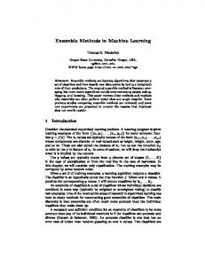
2 Overview of different neural networks architectures Neural networks applied in control loops and safety-critical domains have to meet more requirements than just the overall best function approximation. On the one hand, a small approximation error is required, on the other hand, the smoothness and the monotonicity of selected input-output relations have to be guaranteed. Otherwise the stability of most of the control laws is lost. Three approaches for partially monotonic models are compared in this thesis, namely Monotonic Multi-Layer Perceptron Network (MONMLP) [10], Derivative Bounded Network (DBN) [46], and Constrained Linear Regression (CLR). There has been investigated the advantages and disadvantages of these approaches related to approximation performance, training of the model, convergence and robustness.
2.1 Linear regression 2.1.1 Description and basic equation In statistics, linear regression is a regression method that models the relationship between a dependent variable Y independent variables X i =1.. p and a random term ε . The model can be written as:
Y = β 0 + β 1 X 1 + ... + β P X P + ε
(9)
where β0 is the intercept ("constant" parameter - bias), the βi are the respective parameters of independent variables, and p is the number of parameters to be estimated in the linear regression. Linear regression can be contrasted with nonlinear regression.
2.1.2 Constraints of the model and monotonicity induction In order to induce prior knowledge about the data into training procedure one can use monotonic behavior in input-output relation. Strictly speaking this means that the derivative dY of the output with respect to input is greater than zero ≥ 0 . Constructing Scatter plots (see dX section “monotonicity extraction”) one can extract monotonicity in the data.
2-7
⎧Y = β 0 + β1 X 1 + ... + β P X P + ε ⎪ ⎨ dY ⎪ dX = β i ≥ 0, i = [1; p ] ⎩ i
(10)
It is clear that fixing the coefficients in front of inputs, it is very simple to induce monotonic behavior in input-output relation.
2.1.3 Convergence The convergence of the CLR is presented in figure 3. There is no problem in computing the feasible start point (see eq. 10), since taking β i ≥ 0 one can immediately satisfy monotonicity inequalities.
Fig.3. Convergence of the CLR versus the number of epochs.
2.2 Feed forward neural network 2.2.1 Description and basic equation This class of networks consists of multiple layers of computational units, usually interconnected in a feed forward way. Each neuron in one layer has directed connections to the neurons of the subsequent layer. In many applications the units of these networks apply a hyperbolic tangent function as an activation function (see fig.4).
2-8
Fig.4. Feed forward network, namely MLP is shown in the figure. Here X are inputs, W are weights between layers, Y are outputs. Connections between nodes are presented with the lines. One can see activation functions within dotted rectangulars. Solid numbers display the layer number. In the present work hyperbolic tangent activation function was used. In principal one can use some nonlinear function ( f ⊂ C 2 ) as activation function, but the nonlinearity is principal, due to the fact that linear combination of linear functions is still linear function and linear function cannot process data in the nonlinear way. So far nonlinear hyperbolic tangent function usually is used since it is differentiable and has two saturation limits. General equation of MLP is given in eq.3: ⎞ ⎛ ⎟ ⎜ R ⎛ ⎞ ⎛ 6447448 ⎞ ⎟ ⎜ ⎜ h4 ⎟ ⎜ h2 ⎟ n h4 1 4, 6 2, 4 0, 2 3 5⎟ ⎜ ⎜ ⎟ (11) Y = ∑ ∑ wk tanh ∑ wk ,l tanh⎜ ∑ wi ,m X i + wm ⎟ + wl + w ⎟ ⎜ ⎜ l =1 ⎟ ⎜⎜ m =1 ⎟⎟ i =1 k =1 ⎜ ⎟ ⎟ ⎜ ⎝4 ⎠ 44 ⎝144444 ⎟ ⎜ 4244444 3⎠ Q ⎠ ⎝ th Where n – is a number of inputs, h4 – number of nodes in 4 layer, h2 – number of nodes in 2nd layer. The universal approximation theorem for neural networks states that every continuous function that maps intervals of real numbers to some output interval of real numbers can be approximated arbitrarily closely by a multi-layer perceptron with just one hidden layer. This result holds only for restricted classes of activation functions, e.g. for the hyperbolic tangent functions.
2.2.2 Natural constraints of the model (with different activation functions) To compute natural constraints one should look more precise on eq. 11. Due to the hyperbolical activation function eq. 11 is constrained. Taking into account lim (tanh ( x )) = ±1 x → ±∞
it is possible to say that the maximum possible output of the network is
2-9
n ⎛ h4 ⎞ Y = ∑ ⎜ ∑ wk4, 6 + w 5 ⎟ . On the other hand the derivative of the network has constrained i =1 ⎝ k =1 ⎠ 1 = 1 − tanh( x) 2 , the derivative is limited due to its nature. See fig. 5. function y = 2 cosh( x)
Fig.5. Activation functions for the MLP and their derivatives. To constrain the model with expert knowledge one should induce prior knowledge about the problem. Let’s say that one knows that the input – output relation has monotonic growing behavior, what means that the constraints can be presented like following (see eq. 12): dY (12) >0 dX k One can compute such derivative for eq.11 and obtain eq.13: h2 h4 ∂Y = ∑ wk4, 6 (1 − tanh 2 (Q) )∑ wk2,,l4 (1 − tanh 2 ( R) )wi0,,m2 ≥ 0 14 4244 3 l =1 14 4244 3 ∂X k k =1 (13) >0 >0 if wi0,,m2 wk2,,l4 wk4, 6 ≥ 0 Eq.13. provides sufficient constraints to guarantee monotonicity in I/O relation. Overall problem is shown in eq. 14 n ⎛ h4 ⎧ ⎞ ⎛ h 4 2, 4 ⎛ h 2 0, 2 1⎞ 4, 6 3⎞ 5 ⎪Y = ∑ ⎜⎜ ∑ wk tanh⎜⎜ ∑ wk ,l tanh ⎜ ∑ wi ,m X i + wm ⎟ + wl ⎟⎟ + w ⎟⎟ i =1 ⎝ k =1 ⎝ m =1 ⎠ ⎪ ⎝ l =1 ⎠ ⎠ ⎪ dY ⎪ (14) = wi0,,m2 wk2,,l4 wk4,6 ≥ 0 ⎨ dX k ⎪ ⎪ dY ≤ 1, ∀k = [1; ni ] ⎪0 < dX k ⎪⎩
2.2.3 Convergence On the figures below (see fig. 6) one can find “Functional value” label. This is the error functional (Target - Output of the network)2 constructed while training the neural network. All figures were provided for the “Abalone” benchmark dataset. One shouldn’t pay attention to the initial functional values, since different number of hidden neurons was used in order to
2-10
show possible outcomes. Typical pictures for the MONMLP convergence in case different start points are shown in figure 6.
Fig.6. Convergence of BDN and MONMLP for different start points As one can see in the figure 6 the convergence for MONMLP is not guaranteed in case infeasible start point. The final error for the MONMLP does not depend very much on the weights initialization (in case feasible start point). For MONMLP the situation is worse, since in case optimization starts from infeasible start point, one can see absence of convergence. In order to start from a feasible start point, one can compute feasible start point for MONMLP. In case MONMLP feasible start point for MONMLP can be computed like following: If wi0,,m2 wk2,,l4 wk4,6 ≥ 0 then any positive combination of weights will provide feasible start point and more over monotonicity can be fixed by the signs of weights in the initial layer ( wi0,m, 2 ) in case other weights are fixed as positive ( wk2,,l4 wk4,6 ≥ 0 ). Following the work [10], the impact of the monotonicity conditions is analyzed. The fourlayer feed forward network is an extension of a three-layer standard MLP. Since the threelayer topology is already sufficient for an universal approximator, the extension by a monotonic second hidden layer to a four-layer network respectively additional calculations by hyperbolic tangents and the multiplications with positive weights wk4, 6 do not affect this property Limitations in the sign of the weights wk2,l, 4 can be eliminated by appropriate weights wi0,m, 2 since tanh( x) = − tanh(− x) . To sum up, a four-layer feed-forward network under the
constraints in equation (14) continues to be a universal approximator.
2.3 Integral of feed forward neural network: BDN 2.3.1 Description and basic equation Following the work [46] the derivative of a neural network is typically a Gaussian shaped distribution function which decays to zero at its limits. This means that whenever a neural network starts to extrapolate (or interpolate into sparse data regions), the model derivative (i.e. the process gain predictions) naturally decay to zero (see. fig.4). This results in an intrinsic propensity to under predict process gains which would result in large controller gains and a highly unstable control solution. Since these problems are architecturally intrinsic to neural networks, they have no place in influencing controller behavior over some process
2-11
As a result of the disappointing capability of neural networks in transition control, a universal approximating algorithm was searched for that could not only universally approximate, but could also provide the following essential properties for a predictive control model: 1. Guaranteed monotonicity between inputs and outputs if required. 2. Global limits on its process gain predictions 3. Guaranteed global reversibility 4. Intelligent, elegant and robust extrapolation capability (more importantly interpolation capability into sparse data regions) 5. Universal approximating capability 6. Nonlinear dynamic modeling capability. 7. Directional dependent nonlinear dynamic modeling capability.
These are seven salient properties of the State Space Bounded Derivative Network. The Bounded Derivative Network (BDN) is essentially the analytical integral of a neural network. One should integrate equation 11 in order to obtain BDN –Bounded Derivative Network. For graphical visualization see fig.7 below.
Fig.7. Feed forward network, namely bounded derivative network is shown in the figure. Here X are inputs, W are weights between layers, Y are outputs. Connections between nodes are presented with the lines. One can see activation functions within dotted rectangulars. Solid numbers display the layer number. After integration one can obtain eq. 15 which represent new type of architecture which is called derivative bounded network (BDN [46]). n ⎛ ⎛ ⎛ ⎞⎞⎞ ⎜ ⎜ log⎜ cosh⎛⎜ w 3j ,,11 + ∑ w 3j ,,i2 wi0,i, 2 X i ⎞⎟ ⎟ ⎟ ⎟ ⎟ n h ⎜ ⎜ ⎜ i =1 ⎝ ⎠⎠⎟⎟ Y = w16,1,1 + ∑ w16,i, 2 wi2,i,0 X i + ∑ w16,,j5 ⎜ w 5j ,, 4j ⎜ ⎝ ⎟⎟ n l =1 j =1 ⎜ ⎜ + w 5,3 ⎛⎜ w 3,1 + w 3, 2 w 2,0 X ⎞⎟ ⎟⎟ ∑ j, j j ,1 j ,i i ,i i ⎜ ⎟⎟ ⎜ i =1 ⎝ ⎠ ⎝ ⎠⎠ ⎝
(15)
2-12
where h stands for the number of nodes in 4th layer. For more information one can refer to [46].
2.3.2 Natural constraints of the model To compute natural constrains of the DBN model one should look at figure 6. The activation function of this network is bounded from one side by its nature. This means that dY > 0 . On the other hand its unlimited if X k goes to infinite value. The derivative of the dX k DBN activation function (see. eq. 16 and fig.8) is limited due to the limitation of hyperbolic tangent function. Following the idea one should calculate the constraint, which can take into account monotonic behavior. To do it, one should use eq.7: h n ⎛ ⎛ ∂Y ⎛ ⎞⎞⎞ = wk2,,k0 ⎜⎜ w16,,k2 + ∑ w16,,j5 w 3j ,,k2 ⎜⎜ w 5j ,,3j + w 5j ,, 4j tanh⎜ w 3j ,,11 + ∑ w 3j ,,i2 wi2,i, 0 X i ⎟ ⎟⎟ ⎟⎟ ∂X k j =1 i =1 ⎝ ⎠⎠⎠ ⎝ ⎝
(16)
Then it is possible to see that eq. 16 is bounded by its nature due to the limitation of the hyperbolic tangent function. Eq.16 is very similar to the eq. 11 – general equation for multilayer perceptron. Taking into account that lim (tanh( x )) = ±1 one can obtain eq.17: x → ±∞
∂Y ∂X k
bound
h ⎞ ⎛ h = wk2,,k0 ⎜⎜ ∑ w16,,j5 w 3j ,,k2 w 5j ,,3j ± ∑ w16,,j5 w 3j ,,k2 w 5j ,, 4j + w16,,k2 ⎟⎟ j =1 ⎠ ⎝ j =1
Depending on the sign of the wk2,k, 0 derivative
∂Y ∂X k
(17)
can be maximum (further max) or bound
minimum (further min) bound. In the present thesis assume wk2,,k0 > 0 . Then the derivative lies
∂Y ∂Y < max ⇒ if > 0 then min > 0 . To constrain the ∂X k ∂X k model derivative minimal value for the derivative should be greater then zero. In the figure 8 one can find visualization of the activation function for the BDN network and the visualization for the activation function for the MONMLP network. in some bounded region: min
0, if >0 j ,k j, j j, j 1, j 1, k (18) ⎨∑ ∂X k j =1 ⎪ ⎪wk0,,k2 > 0 ⎪ 6 , 5 3, 2 5 , 4 ⎪⎩w1, j w j ,k w j , j > 0, ∀j = [1; nh] ∂Y > 0 ) one should In order to fulfill eq. 18 in case inputs have ascending behavior ( ∂X k initialize weights according to eq.19:
(
)
(
)
2-14
⎧ 5,3 w16,,k2 ⎪ w j , j = − 6 , 5 3, 2 w1, j w j ,k ⎪ ⎪ 0, 2 ∀j = [1; nh] ⎨ wk , k > 0 ⎪ 6 ,5 3, 2 5, 4 ⎪w1, j < 0, w j ,k > 0, w j , j < 0 ⎪ ⎩ Eq. 12 clearly shows how to start from a feasible start point for BDN.
(19)
2.4 Recurrent neural network 2.4.1 Description and basic equation The human brain is to some extent a recurrent neural network (RNN) [52]: a network of neurons with feedback connections. It can learn many behaviors, sequence processing tasks, algorithms, programs that are not learnable by traditional machine learning methods. This explains the rapidly growing interest in artificial RNNs for technical applications: general computers which can learn algorithms to map input sequences to output sequences, with or without a supervisor. They are computationally more powerful and biologically more plausible than other adaptive approaches such as Hidden Markov Models (no continuous internal states), feed forward networks and Support Vector Machines (no internal states at all). Problem solved with RNNs include adaptive robotics and control, handwriting recognition, speech recognition, keyword spotting, music composition, attentive vision, protein analysis, stock market prediction, and many other sequence problems. Early RNNs of the 1990s could not learn to look far back into the past. Their problems were first rigorously analyzed on Schmidhuber's RNN long time lag project by his former PhD student Hochreiter (1991). A feedback network called "Long Short-Term Memory" (LSTM, Neural Competition, 1997) overcomes the fundamental problems of traditional RNNs, and efficiently learns to solve many previously unlearnable tasks involving: 1.Recognition of temporally extended patterns in noisy input sequences 2.Recognition of the temporal order of widely separated events in noisy input streams 3.Extraction of information conveyed by the temporal distance between events 4.Stable generation of precisely timed rhythms, smooth and non-smooth periodic trajectories 5. Robust storage of high-precision real numbers across extended time intervals The representation of the recurrent neural network is shown in figure 10.
2-15
Fig.10. Recurrent network. Here X i are inputs, Yk are outputs, Wks are synaptic weights. Connections between network layers are denoted by strait lines and feedbacks of information processing are denoted by loops with arrows. The Elman neural network we consider here has the following architecture. It is a feedforward network with three layers: an input layer, a hidden layer, and an output layer (see Figure 11 below). This type differs from conventional ones in that the input layer has a recurrent connection with the hidden one (denoted by the dotted lines (marked as “weight U”) in the Figure 11). Therefore, at each time step the output values of the hidden units are copied to the input ones, which store them and use them for the next time step. This process allows the network to memorize some information from the past, in such a way to better detect periodicity of the patterns.
Fig.11. Elman recurrent neural network. Connections between layers are presented with the lines. “Copy(delayed)” stands to show that networks make the copy of the hidden layer and present it with some weights on the next iteration of the training. In the original experiments presented by Jeff Elman so-called truncated back propagation was used. This basically means that y j ( y − 1) was simply regarded as an additional input. Any
error at the state layer (marked as “Previous state” in the fig. 11), δ j (t ) , was used to modify
weights from this additional input slot (see Figure 11). Errors can be back propagated even further. This is called back propagation through time (BPTT; see fig. 12) and is a simple extension of what one has seen so far. The basic principle of BPTT is that of “unfolding.” All recurrent weights can be duplicated spatially for an arbitrary number of time steps, here referred to as τ . Consequently, each node which sends activation (either directly or
2-16
indirectly) along a recurrent connection has (at least) τ number of copies as well (see Figure12).
Fig.12. Back Propagation Through Time network. Connections between layers are presented with the lines.
Errors are thus back propagated according to rule δ pj (t − 1) = ∑ δ ph (t )u hj f ′( y pj (t − 1)) where m h
h is the index for the activation receiving node and j for the sending node (one time step back). This allows us to calculate the error as assessed at time t, for node outputs (at the state or input layer) calculated on the basis of an arbitrary number of previous presentations.
2.4.2 Natural constraints of the model Due to the fact that during training of the Elman network back connections are ignored, constrains and training procedure are the same, as for feed forward network.
2-17
2.4.3 Convergence The convergence for the RNN, namely Elman Network is quite fast, in case one provides sufficient number of hidden nodes, since training procedure requires gradients and having back connections one can compute only some approximation for these gradients.
Fig.13. MSE decay for the RNN versus the epoch number
Constraints for the derivatives and the start point can be computed in the same way as for MONMLP.
3 Approximation results and approaches to improve quality of the prediction 3.1 Training parameters and results for benchmark data For the training of the MONMLP and BDN Sequential Quadratic Programming (further SQP) technique was used. The implementation of the SQP was done by Optimization toolbox, Matlab. For the training of the RNN Broyden – Fletcher-Goldfarb-Shanno (further BFGS) algorithm was used. Due to the fact that all datasets (except DJIA) were not time series, for the cross validation randomly chosen points were used. Each network (CLR, MONMLP and BDN) was used 10 times for the same data set to find the range for the RMS and R2. The architecture was chosen to be like following: for the MONMLP one should use 8 to 4 units in first hidden layer and 4 to 3 units in second layer, for the BDN one should use 1 to 4 units in hidden layer. For each data set number of epochs was chosen to be 400. Moreover early termination for the training procedure was used. Early termination means that in case the error on the test set starts ascending (after it was descending) and at the same time error on the training set continue descending, one should stop training procedure. To estimate the quality of the result one should use two measures, namely Root Mean Squared Error (RMS) and R2 which is a statistic that will give some information about the goodness of fit of a model. In regression, the R2 coefficient of determination is a statistical measure of how well the regression line approximates the real data points. An R2 of 1.0 indicates that the regression line perfectly fits the data (see eq. 20).
3-18
R
2
2 ( x−~ x) = 1− , where ( x − x )2
x - is a real value, x - is an average value over all real values, ~ x - is
a value obtained in the experiment. All data was normalized according to it’s min and max values. Therefore all data is concentrated between -1 and 1. In the table 1 the best results is marked with the bold script. Table 1. Results for the benchmark datasets. Cross validation RMS Dataset CLR MONMLP BDN ABALONE 0.1 0.14 0.14 CD ARM 0.07 0.07 0.07 BOSTON HOUSING 0.13 0.39 0.13 DJIA 0.07 0.07 0.07 STEEL 0.10 0.15 0.10
Cross validation R2 RNN CLR MONMLP BDN RNN 0.09
-0.01
0.12
0.15
0.36
0.08
0.95
0.96
0.96
0.97
0.14
0.48
0.20
0.48
0.42
0.07
-2.11
-1.29
-0.94
-1.1
0.06
0.91
0.86
0.93
0.97
In the table 1 one can find numerical results for the given datasets. One can see that in most cases RNN would be the best choice in case universal network is needed.
3.2 Approaches to improve quality of the prediction using Empirical Mode Decomposition. From the table 1 it is clear that there is a lot of place for the improvement of the forecast and approximation quality. Therefore several methods have been suggested how to improve the quality of NN approximation.
3.2.1 Introduction to EMD The Empirical Mode Decomposition was invented by Huang [11-16], for the adaptive representation of non stationary signals, as a sum of AM-FM components with zero mean. The basis of the method is in taking into account the oscillation in a signal on a local level. If to look on the oscillations in a given signal x(t) between two extremums (or, two minima in tand t+ ), it is possible to evaluate the high frequency component {d (t ), t − ≤ t ≤ t + } or a so called, local detail, which is responsible for the oscillation, which connects two minima and path throw maxima, which always exist between two minima [6]. To fulfill the picture we have to determine low frequency component with respect to high frequency component m(t) or, the so called, trend. So far we have represented initial signal as a sum of high frequency and low frequency components: x (t ) = m(t ) + d (t ); t − ≤ t ≤ t + Making this procedure several times we can extract finite number of details. For the concrete algorithm see below: Algorithm for mode extraction: 1. Define the local Extremums of the initial signal x(t) 2. Interpolate (with cubic splines) between minima and maxima and build envelopes emin(t) и emax(t) e + emax 3. Compute the average m(t ) = min 2 4. Extract the detail d(t)=x(t)-m(t)
3-19
5. Repeat the procedure for the rest m(t) IMF 1; iteration 1 1.5 1 0.5 0 -0.5 -1 -1.5 10
20
30
40
50
60
70
80
90
100
110
120
70
80
90
100
110
120
residue 1.5 1 0.5 0 -0.5 -1 -1.5 10
20
30
40
50
60
Fig.14. Visualization of the algorithm. 3(а) – an average of two envelopes. 3(b) – residue after subtraction. In practice this procedure leads to sifting process, which leads to the loop of algorithm until we will not have zero average, with respect to some termination criterion [12]. When the average is zero we call the rest “Intrinsic Mode Function” (further IMF, important mode). After this done we make the last step of the algorithm. Thus we have finite number of extrema the procedure is also finite and the number of IMF’s is also finite. Notice that in case harmonic oscillations high frequency against low frequency, EMD should be used in local scale and does not fit to some band filtering. The procedure described above is fully automatic and adaptive. The example is shown below (see. fig. 15). In the figure 15 one can see the scheme how we obtained noised signal. In the figure 16 one can see the results of empirical mode decomposition [11-16].
3-20
Fig. 15. Scheme how to obtain noised signal. We took the tone, then added some chirp and thus obtained noised signal
res.
imf6
imf5
imf4
imf3
imf2
imf1
Empirical Mode Decomposition
10
20
30
40
50
60
70
80
90
100
110
120
Fig. 16. Empirical mode decomposition for noised signal. We extracted two modes (imf1 and imf2). The rest modes can be considered as equal to zero. One can see that the decomposition was quite successful Interpolation and border effects. In order to approximate upper and lower envelopes the best idea is to use cubic splines [12]. Extrema must be extracted very accurate and this leads to over discretization. Border effect must be taken into account, in order to minimize the error at the ends of time series, which appears due to finite number of points in the time series. So far we have to add Extremums which not exist. This help fighting against border effects making it smaller. More information one can find in [11-16].
3-21
3.2.2 Combination of inputs The traditional approach at neural forecasting is based on immersing of time series in lagged space. Thus, it is considered that we restore or we reconstruct phase attractor of the dynamical system inside a neural network and thus we extract laws of development of system in time (see Taken’s theorem). In the present thesis we assume that development of some asset is «almost Markov» process. (In other words, Markov process is a process where "future" of process does not depend on "past" at known "present"). The word "almost" means that tomorrows value of some asset depends mainly on today's value, but, nevertheless, also depends and on the previous values.
Fig.17. Visualization for the Altria Group Inc (MO) share price behavior Thus, in our approach for the input of a neural network we present the combination of value obtained during the last 5 days but with different weights. Thus there is a following problem. Having one input (or several correlating, notice that lagged vectors will correlate) neural network will have so-called «information famine». On the other hand, one input it is not enough to approximate time series by means of neural network. To overcome this difficulty it is necessary to extract as much information as possible from only one time series. For this purpose it was suggested to use EMD method. The given modes will possess orthogonal properties [12], and the number of modes will be about 9 to 12 modes. Thus we obtain 9-12 not correlating and orthogonal inputs. If to do the given procedure for investigated time series, we shall notice that in the pure state low frequency modes will strongly dominate in comparison with the others (see fig.18). Moreover, a priori we know that low-frequency components form a trend of time series and this trend cannot be removed from decomposition, because this will affect border effects, as well as others cannot be neglected. Subtraction of modes leads to strong boundary effects and, thus, the forecast even for 1 day to become impossible because we have to move in the past on number of steps equal to size of boundary effect.
3-22
Fig.18. Comparison of the modes in the signal. Around each “mode number”the development of the mode in time is presented. On color picture this development in time is presented with color gradient. Thus, it is necessary not to influence the signal in artificial way but all inputs must be of the same value in average. For this purpose in the present work it was suggested to extract modes not for the initial signal, but for the derivative of a signal. New representation of the signal allowed us to reduce influence of low frequency component and made all inputs of the same order (see. fig.19).
Fig.19. Comparison of the derivative of the modes displayed in fig. 18. Around each “mode number”the development of the mode in time is presented. On color picture this development in time is presented with color gradient. Now, to illustrate the computational error of EMD method, we compute the sum of all modes and subtract this sum from the initial signal. The result is shown in figure20.
3-23
Fig.20. Difference between sum of modes and initial signal From the figure 20 one can see that the error of the order 10-16 is insignificant. Notice that if we add new points to the time series, uniqueness of decomposition is broken, since modes become others, and it is necessary to retrain ANN at each time as soon as new value is received. For comparison: time for training of the network for a computer in Matlab environment (CPU: Celeron 1.3 RAM: DDR2 2Gb) takes 5 minutes, and decomposition of a signal on modes takes 30 seconds. On the other hand, for operative forecasting for 1 day this time of training is absolutely not critical. As the process we are dealing with is not purely Markov one it is necessary to deliver also some number of weighted lagged vectors. Thus for the input of a neural network we have modes in current day, and also some set of lagged vectors. For the output of a neural network we present the future value of a derivative of the time series we are working on. Results of investigation are the following. For carrying out of experiment we took the data Dow Jones index. For carrying out the experiments the committee of recurrent Elman networks (the result of committee was simple averaging over answers of all networks) was used. We used two layers of neurons (10 neurons in each layer). The important feature of recurrent networks is the method for the optimization of weights (a method of training). In the present work the method of optimization under name BFGS was applied. As functions of activation hyper tangential functions of activation were used.
3-24
Fig.21. Inputs of the NN. Here 9 modes of the initial signal (inputs 1-9) and 6 lagged signals made of (10-15) of the initial signal are presented. For more information one can refer to [54].
3.2.3 Results The results of applying ANN for the generalization set are shown in table 2 and in figure 22.
Fig.22. Forecast for one time step. Comparison of forecast and reality In the table 2 there is a comparison of two forecasting techniques. The first technique is a so called technique of lagged vectors (further TDNN – Time Delayed Neural Network) where
3-25
for the inputs we present a set of lagged (in time) vectors, and for the output we simply present the future value. The second technique is a technique which is described in the present work. The data mentioned above was normalized to the interval from 0 to 1. Results of such comparison are presented in table 2: Table 2. Comparison of the results for two different forecasting methods Comparison of two methods New method Method of lagged (generalization set) vectors (generalization set) 2 Determination coefficient (R ) 0.92 0.7 Correlation coefficient (r) 0.95 0.92 Root Mean Squared Error 0.08 0.13
From the table 2 it is easy to see that the EMD approach has influenced the forecast. Moreover this influence has caused better ability for the generalization (see R2) and approximation capabilities (see RMS, r).
3.3 Appropriate training for ANN to induce some a priori rules into the inner structure of the ANN. 3.3.1 monotonicity extraction In order to induce monotonicity for some inputs from input space one should mine monotonic behavior from the data. The acquisition of the monotonic behavior can be divided into two parts. First one is context acquisition, which means that one should extract monotonicity from deep understanding of the process he or she is dealing with. Second possibility is the extraction of the prior knowledge from the data using scatter plots. Using scatter plots one can see monotonic behavior in input-output relation. An example one can see in figure 23 below.
Fig.23. Scatter plot of the data. Output vector against input vectors From the figure 23 one can see monotonic (increasing) behavior between let’s say 3rd input and output. One can use this information in order to introduce constraints. Looking at the figure 1 one can obtain eq.1: ∂Y >0 (21) ∂X k =3 This idea was already used in the sections where constrains for MONMLP, DBN and CLR were introduced.
3-26
3.3.2 Constrained learning In order to show how powerful constrained networks operate, it was decided to compare performance of each constrained network on benchmark datasets. To estimate the quality of the result one should use two measures, namely Root Mean Squared Error (RMS) and R2 which is a statistic that will give some information about the goodness of fit of a model. In regression, the R2 coefficient of determination is a statistical measure of how well the regression line approximates the real data points. An R2 of 1.0 indicates that the regression line perfectly fits the data (see eq. 20). 2 ( x−~ x) 2 , (20) R = 1− ( x − x )2 where x is a real value, x is an average value over all real values, ~ x is a value obtained in the experiment. The results of the study are presented below. All data except last two rows was taken from De Moor B.L.R. (ed.), DaISy: Database for the Identification of Systems, Department of Electrical Engineering, ESAT/SISTA, K. U. Leuven, Belgium, URL: http://www.esat.kuleuven.ac.be/sista/daisy/. For the training of the Monotonic Multy Layer Perceptron (further MONMLP) and Bounded Derivative Network (further BDN) Sequential Quadratic Programming (further SQP) technique was used due to the constrained optimization procedure required. The implementation of the SQP has been done by Optimization toolbox, Matlab. For the training of the RNN Broyden – Fletcher-GoldfarbShanno (further BFGS) algorithm was used. Due to the fact that all datasets (except DJIA) were not time series, for the cross validation (testing) some data points were randomly chosen and then used. Each network (CLR, MONMLP and BDN) was used 10 times for the same data set to find the range for the RMS and R2. The architecture was chosen to be like following: for the MONMLP one should use 8 to 4 units in first hidden layer and 4 to 3 units in second layer, for the BDN one should use 1 to 4 units in hidden layer. For each data set number of epochs was chosen to be 400. Moreover early stopping for the training procedure was used. Early stopping means that in case the error on the test set starts ascending (after it was descending) and at the same time error on the training set continue descending, one should stop training procedure.
3.3.3 Results In the table below (see table 3) one can find results for each dataset. All data was normalized according to it’s min and max values. Therefore all data is concentrated between -1 and 1. Table.3. Comparison of the results for each dataset. Dataset Cross validation RMS CLR MONMLP BDN ABALONE 2.45 ± 0.05 2.3 ± 0.05 2.0 ± 0.7 CD ARM 0.10 ± 0.00 0.09 ± 0.00 0.09 ± 0.00 BOSTON 9.1 ± 0.3 3.80 ± 0.2 3.30 ± 0.4 HOUSING DJIA 56.80 ± 0.1 31.0 ± 1.0 31.5 ± 0.5
Cross validation R2 CLR MONMLP 0.4 ± 0.1 0.53 ± 0.8 0.87 ± 0.01 0.90 ± 0.00 -1.9 ± 0.2 0.45 ± 0.15
BDN 0.37 ± 0.1 0.90 ± 0.00 0.4 ± 0.1
0.37 ± 0.02
0.45
0.45 ± 0.05
± 0.1
3-27
STEEL
118.10 ± 2.10
22.60 ± 2.0
22.70 ± 2.0
0.07 ± 0.03
0.96 ± 0.01
0.96 ± 0.01
Average Variance
± 0.45
± 0.55
± 0.61
± 0.12
± 0.18
± 0.06
From the table 3 one can see that induction of the constrains influenced the forecast. Moreover it is clear that this influence is negative with respect to generalization and approximation capabilities (see table 1). The only thing one should notice that such type of neural networks guarantees monotonicity for the input-output relation by the structure (see sections 2.1, 2.2 2.3). This is very important for some industrial applications and therefore we can pay for this achievement with generalization and approximation capabilities.
3.4 Feature extraction for increasing forecasting horizon: reconstruction of time series from one Fourier spectrum. 3.4.1 Feature extraction idea In this section data preprocessing and the preparation of the inputs for the forecasting and classification algorithms are discussed. According to the work [55], it is a very important and challenging problem. Let us divide given time sequence T into the set of equidistant sub sequences { ti } so that the ) time interval between them is equal to t . For the generalization of presented approach this procedure corresponds to the process of collecting the number of measurements periodically. It should be mentioned that dealing with a limited amount of measurements one should always remember about the tradeoff between how far one wants to forecast (it would be shown that it is related to the time interval between consequent measurements) and how many patterns one needs to make the prediction. For every subsequence ti the Fourier spectrum Fi is computed. Having the set of “consequent” Fourier spectra {Fi }i =1, N the frequency dynamics, if any, could be observed. So that the monitoring of the important changes in signal frequency characteristic over the time can be done. This approach is related to the time frequency analysis (see fig. 24). Each of the obtained spectra could be used for analysis of the bearing conditions for the corresponding time interval. The idea here is to do forecasting in order to get the estimation of future spectral characteristic. In order to do it the particular frequency component changes over the sequence of spectra would be considered.
3-28
Fig.24. Data preprocessing stage illustration. One the top of the figure one can find the representation of the signal and it’s development in time, then in the middle one can see the procedure of the dividing the initial signal T into subsequence of the signals {tj} and then for each subsequence one can compute the Fourier spectra {Fj}. The problem is that the spectrum itself contains too many data and, moreover, not all these data are used for particular faults detection. Therefore it would be consistent to extract few features of the great importance regarding the particular type of fault from the overall frequency data set and to do forecasting only for them (see fig.25.). As a possible feature here an analogue of a crest factor measure C kj (see eq.21) can be used. C kj =
{fi } peak value max = iW , j = 1, M and k = 1, N j RMS 2 ∑ fi
(21)
i =1
Wj
where f i are the frequencies from selected window and M is the number of features for every
{ }
spectrum and N is the number of spectra. For ∀j ∈ [1, M ] values C kj k =1, N form time series ) with a sampling rate inversely proportional to the time interval t introduced above. The overall spectrum feature extraction scheme could be described as a selection of important frequencies (e.g. the defect frequencies or the frequencies of particular interest), choosing an appropriate window around each of the frequencies, and then calculating the mentioned above crest factor analogues values for those windows (see figure 25). Situation when the selected measure is close to 1 corresponds to the absence of peak within the window considered, while relatively high value corresponds to the existence of peak respectively.
3-29
Fig. 25. Feature extraction idea. One should take the Fourier spectrum, compute the RMS (here RMS value) for and the maximum value (the biggest amplitude, here fj and its peak value) inside some window (this is a priori knowledge) and compute Cjk according to the eq. 21.
{ }
Finally as an input for the predictor a set of the time series C kj
k =1, N
is used, each of them
corresponds to the selected particular frequency component j and has a sampling rate, ) defined by the time interval t determined as a gap between two measurements. The aim of this process is to increase the time intervals between the data points, without loosing the important high frequency information. One of the most important restrictions of the scheme presented is that all the measurements should be done within approximately similar conditions, such as rotation speed, external noise etc. Therefore one could expect that the defect growth will be observable within a selected frequency interval. Overcoming of this restriction is theoretically possible and could be considered as one of the further steps to extend the presented approach. An example of the time series C kj k =1, N is shown in the figure 26.
{ }
Fig. 26. Example of features time series we are going to predict, sampling rate 5 sec.
3-30
The approach presented above could be considered as an additional part of the vibration analysis and monitoring system, which allows analyzing the evolution of the particular defect introduced by the bearings components. Together with a suitable measurement strategy it could be used for a considerably long term prediction of frequency characteristics of the vibration signal. While the most of the neural network applications in the field of vibration diagnostic is devoted to the classification problem we have tried to apply it for the forecasting problem. According to the set of experiments it was stated that the proposed technique could be used for the prediction of the introduced frequency features. As a possible extension of suggested approach we could consider including the envelope spectra features forecasting together with some additional measurements (e.g. data from temperature sensors) and some statistical values (e.g. kurtosis, skewness) calculated in the time domain for the subsequences {ti} in order to cover the forecasting of the main characteristics of vibration signal used for the analysis of the equipment conditions. The extension of presented method for the changing rotation speed could be also the thing of a great importance, because it would allow simplifying the data acquisition process. Also it would be possible to extend present approach by extending forecast horizon. It means that following the paper of Kevin Judd, Michael Small [8] we are able to produce forecasts not only for one time step, but also to provide medium-term forecast. That will give us a possibility for medium-term forecasting and middle range control. Then the Empirical Mode Decomposition should be used in order to decompose initial signal into the set of orthogonal and non correlated time series (modes). The sum of the modes is equal to the initial signal (with an error of order 10-16). Let us assume that the next state of the system will depend mainly on the current state of the system and depend also on few previous states with smaller weights (see fig. 27). Therefore, the intrinsic mode functions at the current moment t and the current state of the system with a few lagged intrinsic mode functions (with smaller weights) should be used as inputs for the ANN. The result is shown in the figure 28.
Fig.27. Visualization of all inputs for ANN
As one can see from figure 27, some of the inputs (e.g. #6 and #7) are not of the great importance in comparison with the others. Nevertheless all of them have to be taken into account in order to avoid border effects of EMD method which could be rather strong. Since the next state depends mainly on the current state (according to the assumption above) neural network have to be retrained to maintain the conditions of such specific process and to neglect border effects of EMD filter.
3-31
3.4.2 Results Results of the forecast are presented in figure 28.
Fig.28. One step forecast for the selected feature. The procedure was repeated 30 times to estimate statistical quality of prediction for one step, sampling rate for time axis is 1 day.
As it could be noticed from figure 28 (bottom picture), non delayed forecast for the frequency component development (see table 1) has been obtained. Below the comparison of linear regression and time delay neural network (further TDNN), with the proposed advanced forecasting technique based on RNN (further AFT) is given. Table 4. Comparison of the quality of the forecast provided by different methods.
LR TDNN AFT
r 0,30 0,38 0,66
R2 2 0,06 0,14 0,30
MSE 0,03 0,02 0,01
Table 4 gives a brief overview of the quality of the forecast for the following statistics: mean squared error (MSE), determination coefficient ( R 2 , see eq.2) and correlation coefficient ( r ).
4 One side classifiers According to the works [30-32] condition monitoring is an important and challenging task actual for many areas of industry, medicine and economics. Nowadays it is necessary often to provide on-line monitoring of the complex systems operation conditions, e.g. the steel production, in order to avoid faults, breakdowns or wrong diagnostics. In the present thesis a
4-32
novel machine learning method for the automated condition monitoring is elaborated. Neural Clouds (NC) [56] is a novel data encapsulation method, which provides a confidence measure regarding classification of the complex system conditions. The presented adaptive algorithm requires only the data which corresponds to the normal system conditions, which is typically available. At the same time the fault related data acquisition is expensive and fault modeling is not always possible, especially in case one is dealing with steel production, power stations operation, human health condition or critical phenomena in financial markets. These real word applications are also presented in the thesis. To make picture of one side classifiers complete, we compare NC method with other approaches namely Parzen-Window and Gaussian mixture models.
4.1 Classifier types There are lot of different approaches to the data classification. Here we compare only 3 methods, namely Parzen-Window, Gaussian mixture and NC models..
4.1.1 Gaussian mixture Mixture Models [38] are a type of density model which comprise a number of component functions, usually Gaussian. These component functions are combined to provide a multimodal density. Mixture models are a semi-parametric alternative to non-parametric histograms (which can also be used as densities) and provide greater flexibility and precision in modeling the underlying statistics of sample data. Gaussian mixture models can also be viewed as a form of generalized radial basis function network in which each Gaussian component is a basis function or `hidden' unit. The component priors can be viewed as weights in an output layer. Finite mixture models have also been discussed at length elsewhere [38] although most of this work has concentrated on the general studies of the properties of mixture models rather than developing vision models for use with real data from dynamical scenes. Let the conditional density for a sample data ξ belonging to a data Q be a mixture with M component densities: M
p (ξ Q ) = ∑ p (ξ j )P( j )
(22)
j =1
where a mixing parameter P(j) corresponds to the prior probability that sample data ξ was generated by component j and
M
∑ P( j ) = 1 ,
p (ξ Q) is a conditional density for the data Q, and
j =1
since Q consist of M mixture components, then p(ξ j ) – is the conditional density for each mixture component. Each mixture component is a Gaussian with mean μ and covariance matrix ∑ , i.e. in the case of a 2D data: 1 ⎛ 1 ⎞ T (23) exp⎜ − (ξ − μ j ) Σ −j1 (ξ − μ j )⎟ p(ξ j ) = d ⎝ 2 ⎠ (2π ) Σ j Where Σ j is the covariance matrix for jth mixture component and Σ −1 j Is the inverse covariance matrix for the jth mixture component. The mixture model is simply used for its mathematical flexibilities. For example, a mixture of two normal distributions with different means may result in a density with two modes, which is not modeled by standard parametric distributions (see Fig. 29).
4-33
Fig.29. Gaussian mixture. At the left side 2D contour lines plots are pictured and at the right – normalized density 3D plots. With red circles dataset is presented. Contour lines in 2D and in 3D show the density. In 3D it can be interpreted like the probability (under some normalization to the interval [0 1])
4.1.2 Parzen-window Emanuel Parzen [37] invented this approach in the early 1960s, providing a rigorous mathematical analysis. Since then, it has found utility in a wide spectrum of areas and applications such as pattern recognition, classification, image registration, tracking, image segmentation, and image restoration. Parzen-window density estimation is essentially a data-interpolation technique . Given an instance of the random sample, x, Parzen-windowing estimates Probability Density Function (further PDF) P(x) from which the sample was derived. It essentially superposes kernel functions placed at each observation or datum. In this way, each observation xi contributes to the PDF estimate. There is another way to look at the estimation process, and this is where it derives its name from. Suppose that we want to estimate the value of the PDF P(x) at point x. Then, we can place some window function (function which is non zero for some region of the space, otherwise is zero elsewhere) at x and determine how many observations xi fall within our window or, rather, what is the contribution of each observation xi to this window. The PDF value P(x) is then the sum total of the contributions from the observations to this window. The Parzen-window estimate is defined as 1 n 1 ⎛ x − xi ⎞ ⎟ (24) P( x) = ∑ d K ⎜⎜ n i =1 hn ⎝ hn ⎟⎠ where K(x) is the window function or kernel in the
∫ K (x )dx = 1
ℜ
-dimensional space such that (25)
d
and hn>0 is the window width or bandwidth parameter that corresponds to the width of the kernel. The bandwidth hn is typically chosen based on the number of available observations . Typically, the kernel function K(.) is unimodal. It is also itself a PDF, making it simple to guarantee that the estimated function P(.) satisfies the properties of a PDF. The Gaussian PDF is a popular kernel for Parzen-window density estimation, being infinitely differentiable and
4-34
thereby lending the same property to the Parzen-window PDF estimate P(x). Using eq. (25), the Parzen-window estimate with the Gaussian kernel becomes ⎛ 1 ⎛ x − x ⎞2 ⎞ 1 n 1 i ⎟ ⎟ (26) P ( x) = ∑ exp⎜ − ⎜⎜ ⎜ 2 ⎝ hn ⎟⎠ ⎟ n i =1 h 2π d ⎝ ⎠
(
)
where is the standard deviation of the Gaussian PDF along each dimension. Figure 30a shows the Parzen-window PDF estimate, for a zero-mean unit-variance Gaussian PDF, with a Gaussian kernel of and increasing sample sizes. Observe that with a large sample size, the Parzen-window estimate comes quite close to the Gaussian PDF.
Figure 30a: The Parzen-window PDF estimate (dotted curve), for a Gaussian PDF (solid curve) with zero mean and unit variance, with a Gaussian kernel of and a sample size of (a) 1, (b) 10, (c) 100, and (d) 1000. The circles indicate the observations in the sample.
4-35
Fig.30b. Parzen window. At the left side 2D contour lines plots are pictured and at the right – normalized density 3D plots. . With blue circles dataset is presented. Contour lines in 2D and in 3D show the density. In 3D it can be interpreted like the probability (under some normalization to the interval [0 1])
4.1.3 Neural Clouds The Neural Clouds (NC) concept was successfully elaborated and applied by the Corporate Technology Department of Siemens AG for solving the steel production optimization problem [56]. However this technique has been also transferred, with the necessary modifications, to the field of vibration analysis [4], EEG classification and financial market analysis and prediction. The application of these neuro-fuzzy methods, presented in this thesis, makes the expert condition monitoring system more intelligent and able to face the real world problems, keeping the monitoring costs reasonable. The concept presented in the thesis is directed for the elaboration an efficient data encapsulation method for the adaptive solving of the so called one-side classification problem. The basic idea behind the usage of the one-side classification in the field of condition monitoring and fault analysis is that the real data, which can be collected, usually corresponds to the normal conditions of the complex systems in question. Vice versa data collection, corresponding to abnormal conditions, is expensive, and fault modeling is not always available. Here one should mention that the idea of elaboration of the classifier based on a data, collected from the system under normal operating conditions, could be extended for the case of the human health-related measurements classification, where the data acquisition related to particular disease is even more problematic. The NC application deals with following problems: analysis of vibration data [30-32], EEG data classification [24-28, 33-36] and prediction of the American stock market declines [3944]. In the following a more detailed explanation of mentioned steps of the algorithm is provided. Data normalization As a first step the data normalization procedure should be performed in order to avoid clustering problems, corresponding to the possible significant difference in data distribution. The Min-Max normalization procedure was chosen, where the minimal value corresponds to minus identity and maximum value to plus identity respectively. An alternative approach is the normalization of the input data assuming a normal distribution diverse input data scaling is a way to modify the sensitivity per dimension. This will effect the calculation of the multidimensional distances for clustering purposes as well as the sensitivity of the final Neural Clouds regarding deviations from “normal” conditions. Clustering The positioning of the radial nodes (“centers” of the data. One should decide how much data should be around the node in some neighborhood to say that this is the radial node) over the input space in such a way, when they represent groups or clusters of inputs vectors, can be carried out by means of any non-supervised algorithm for clustering. In our approach the well known K-Means algorithm [3-4] is adopted and an advanced variation of the K-Means algorithm is proposed (further AKM). The most remarkable enhancement introduced is that the algorithm is able to set the optimal number of centroids between a maximal and a minimal
4-36
bounds defined by the user. AKM make the centroids adaptively according to density and volumetric distribution. AKM itself consists of the next steps: Set an initial number of centroids nh , a maximal and a minimal bound. Call k-means algorithm to position nh centroids. Insert or erase centroids according to the following premises: If the distances of data are above a certain distance from the nearest centroid, then generate a new centre. If any cluster consists of less than a certain number of data, then remove the corresponding centroid. If the distance between some centroids is smaller than a certain value, then combine those clusters to one. Loop to step 2 unless a certain number of epochs is reached, or centroids number and their coordinates became stable.
AKM algorithm visualization convergence is presented in Fig. 31.
Fig.31. Visualization of the AKM convergence. The growth of the number of center with respect to number of algorithm iterations and its saturation is shown with red circles on the left hand side. The decay of the RMS distance from the center to the data point center with respect to number of algorithm iterations and its saturation is shown with green circles on the right hand side. In the figure 31 one can see that after 6 epochs the number of centroids (data centers) have reached saturation, which means that there is no need to continue searching for new data centers. Looking to the RMS distances it is obvious that this value has saturation after 6 epochs which means that founded centroids are optimal. Application of Gaussian bells After all centroids have been extracted from the input data, the data should be encapsulated with the some smooth hyper surface. To construct this surface Gaussian distributions – so called “Gaussian bells” – are used [2]:
Ri ( x) = e
−
x − mi 2σ
2
2
(27)
4-37
where mi is the centre of the Gaussian bell and σ is the width of the Gaussian bell. The centroid of the AKM cluster becomes the center of corresponding Gaussian bell. Each cluster is covered with the corresponding Gaussian bell. A constant width per dimension is selected in order to avoid side-effects, related to the subsequent normalization. Normalization of the Gaussian bells The sum of all Gaussian bells is provided in order to obtain the encapsulating surface. It may be more than unity – in case these bells have cross sections (see Fig 32). Therefore, normalization similar to the partitioning-to-one known for radial-basis function networks should be performed as far as those values would be used as probability measures with values between 0 and 1. Applying the partitioning-to-one approach, however, leads to the value 1 overall the input space. An additional factor g 0 is introduced (see eq. (28)).
Fig.32. Normalization effects with g 0 . The influence of the g 0 is discussed below As a first step of the Gaussian bells normalization let us perform the data outliers determination. For this purpose let us construct the supplemental Gaussian bells for every data point from the given set. Summing up the values of all Gaussian bells for given data set, values represented in Fig. 33 could be obtained. This information enables to determine the bias factor g 0 , represented by the horizontal line, e.g. by setting it equal to the value, which corresponds to the first percentile of all sums of Gaussian bells ( or sums of values of Radial Basis Functions (further RBF)). The underlying assumption is that the encapsulation of outliers should be avoided in order to obtain plausible results for the Neural Clouds.
4-38
Fig.33. Robust selection of the normalization factor g 0 . The normalized data encapsulator is defined as: n
Pc ( x ) =
∑
i =1
n
∑
i =1
Ri (x)
Ri (x) + g
,
(28)
0
where R i ( x ) are the Gaussian bells, as defined by (27), and g 0 is a global factor, described above. Figure 34 shows the g 0 influence to the final width of the encapsulator. Given input x as a matrix of inputs (patterns) and the output will be a vector of confidence levels, calculated for each element. Different sets of parameters g 0 , σ and the number of AKM clusters n are responsible for the adaptation of the NC to the given data set and determining different tolerance levels. As a possible extension of the presented approach we consider the automation of the mentioned above values selection. However, not all information for these parameters could be extracted out of the given data set. Sensitivity per dimension, the noise level in the data and the evidence of outliers in the data is critical information, usually provided by experts. Here, it should be mentioned that this constructed mechanism could be described in a form of Radial Basis Function network [10], as it is shown in figure 34. After such a network is manually trained by tuning mentioned parameters on the measured data, it could be used for the confidence level estimation for the new measurements.
4-39
Fig.34. Radial Basis Function network representation. L1 and L2 are Layer one and Layer two respectively. X1..k are input patterns and Pc is a confidence value for the concrete pattern X1..k. The output vector, generated by the NC algorithm, is in a form of a confidence value between 0 and 1 that can be interpreted as a measure of the failure probability according to the expression in eq. 29: Pf = 1 − Pc ,
(29)
where Pf is failure probability and Pc is a confidence level. The visualization of the constructed sample NC is presented at figure 35a. On the left side the confidence levels are represented by the contour lines and on the right – by the 3D surface.
Fig. 35a. Left hand side: Classification in 2D space for 2 selected features (normalized density), right hand side: classifier in 3D space (normalized density).
4-40
4.2 Results for benchmark data The advantage of this one side classifier is that it is very flexible to data. Traditional monitoring of the system conditions is based on presenting the thresholds for each value. Typically these thresholds are very simple. NC concept allows creating flexible thresholds which could be adapted to the system. The difference between old approach and new approach is illustrated below.
Fig. 35b. Comparison of hard thresholds with NC concept. Solid line on the left figure stands to show the NC approach (cloud like shape) and thin line stands to show modern simple approach (box like shape). On the right figure NC approach is displayed with smooth surface and nowadays approach is displayed with cubic scratch. Here data is shown with small points, “old” threshold approach is presented with thin line and NC approach is presented with thick line. One can see from the picture that NC suggests more flexible solution than hard thresholds. Below we consider different show cases where it is clearly shown that NC concept can be used in real world applications.
4.2.1 Example for vibration analysis Numerous papers during the last decades were devoted to the vibration analysis problems [30-32]. The main idea behind the traditional approaches is that some particular defects generate the noticeable increase of amplitude on the frequencies which could be calculated from e.g. bearing or gearbox parameters. Implementing amplitudes monitoring within some frequency bands around these frequencies, experts determine, whether this situation corresponds to the normal state of the system or to the fault one [56]. The main difficulty of such approach is the following. For the quite complex systems, where the sensors are measuring the superposition of signals from different sources (e.g. system could contain several different bearings, so that their defect frequencies can overlap each other) and the certain noise, standard methods could not be applied. The present study is focused on development of an evaluation method, which is aimed to perform a diagnosis of rotating machinery without prior knowledge regarding the internal structure of the system and the
4-41
system environment. This evaluation method has to be able to distinguish data, obtained in normal situations, from the critical and abnormal ones. This application of the neuro-fuzzy modeling enables to detect variations from the standard behavior. For this particular application a number of Fourier spectra, measured for the system in normal state, were used for the encapsulating surface (NC) creation. After the so-called training phase, the abovementioned method was used for classification of the succeeding states by computing the confidence values for them.
Fig. 36 Spectral data density contours for Fourier spectrum and corresponding 3D surface for the same spectrum which involves visualization of the probability value. The spectrum peaks generate different alarm levels, which depend on the corresponding confidence level (see Fig.36). If there is a critical change in the spectrum, the confidence level decreases from 100% to 0%. By means of setting the appropriate alarm levels the algorithm (NC) could estimate whether the situation corresponds to the uncritical – good –, critical – warning –, or extremely critical – alarm – states (see Fig. 37). It represents a model to support the human expert in the task of estimating the remaining system lifetime and preventing the breakdowns. Moreover the evolution of the confidence value could be followed during weeks or months if the NC is installed as an on-line monitoring system, performing periodic measurements with a frequency of minute order. This represents a significant stage for the concept of the real time diagnosis system. The developed evaluation method enables the detection of system defects and also the efficient diagnostic of the system (which is under monitoring) “health”.
4-42
Fig. 37 Confidence along measurements for the detection of failures
4.2.2 EEG classification problem Modern electroencephalography uses constantly expanding variety of signal processing algorithms. Along with wide developing of computer systems in last decades this makes it possible to extract more information about brain processes in wide range of studies. Numerous papers on quantitative electroencephalography have been published [24-28]. These studies are very important for understanding the nature of processes in human brain. Nevertheless, inverse problem meets many difficulties. In situations, when it is necessary to make diagnostics of disease, state or peculiarities of the person under study; qualitative methods are still most effective. The main disadvantage of these methods is the neurophysiologist requirement to make qualified subjective assessment of the EEG recording. In addition, subjective assessment cannot be instant and be used in long time monitoring. One of the possible ways to solve this problem is the usage of intellectual classification systems. Their successful development will make it possible to express diagnostics of brain diseases and building of diagnostic, monitoring systems etc. Modern diagnostic systems studies, based on artificial neural networks, show the potential of such methods [24-28]. In present section, we suggest a new approach in this direction. In order to show, how powerful the method can be, we applied this method to the classification of one of the most difficult time series types, namely EEG. Even classification of the EEG recordings is very difficult task. The idea behind the classification is to say whether the EEG belongs to healthy subject or not, or to evaluate the state of the subject during the EEG registration. In present only neurologist can firmly identify EEG fragments, which correspond to abnormal patient’s state, - by subjective evaluation. As the first step, we try to distinguish the EEG of the subject with open eyes from the EEG of the same subject with closed eyes. EEG’s, recorded in these two states, can be easy distinguished subjectively. We used EEGs, recorded from 19 electrodes, placed according to the international 10-20 system [57]. The idea was to build NC (in 19 dimensional space) for the EEG recording of the man with open eyes and then to present the EEG of the same man with closed eyes to the trained NC in order to obtain the answer, whether the new points belong to the NC or not, without inducing the prior knowledge about the EEG time series into the algorithm. Results are presented in the table 5. In the following the “training set” means that some measurements have been randomly taken from the EEG, recorded in the state with open eyes, which was used for the NC creation. “Test set” stands for the projection of the measurements on the NC, which is not used for NC creation, but which corresponds to the EEG, recorded in the state with open eyes. “Generalization set” means that the data, which corresponds to the EEG, recorded in the state with closed eyes, have been projected on NC, constructed using the EEG data, which corresponds to the EEG, recorded in the state with open eyes. “Probability” means that with such probability the measurement, projected on NC, belongs to the EEG, recorded in the state with open eyes. For more details about the computational experiment see table 5.
4-43
Table 5. EEG in states with open and closed eyes. Results are obtained in computational experiment. The field “Number of AKM centroids” emphasizes the sensitivity of this algorithm with respect to this parameter Parameter description Value Number of points which do not belong to the NC when 58% the subject closes eyes (ideal case 100%) Number of AKM centroids 53 Computation time to configure NC (CPU:1.86Ghz, 25 sec RAM: 4 GB DDR2) Evaluation results, number of data point’s, which do not Training Test Generalization belong to NC, ideal case for training set and test would set set set be 0%, for generalization set 100%. 3.8% 7.8% 57.6%
Table 5 shows that investigating the EEG with NC it is difficult to separate open eyes from closed eyes. Nevertheless one can see that the NC usage doesn’t require a lot of time and computational efforts. To make the obtained results more evident, the technique that is mentioned above has been applied for another dataset. These are EEGs, recorded before and during epileptic seizure. They correspond to two different states of the brain (in context of epilepsy). These two kinds of EEG recordings also can be easy distinguished visually. Results one can see in the table 6 below. Table 6. EEG before and after epileptic seizure. Summary of all results obtained in computational experiment. Parameter description Value Number of points which do not belong to the NC when 95.7% the subject is in seizure (ideal case 100%) Number of AKM centroids 60 Computation time to configure NC 65 sec Evaluation results, number of data point’s which do Training Test Generalization not belong to NC, ideal case for training set and test set set set would be 0%, for generalization set 100%. 0.3% 0.93% 95.7%
As one can see from the results above, this method have easily separated the EEG recordings, made before seizure, from the EEG recordings, made during seizure with the probability of 95.7% on the generalization set. This method may be used in clinical practice – EEG (sometime combined with videorecording) long-term seizure monitoring. This diagnostic procedure makes it possible to record EEG during up to 72 hours [57] and is useful when epileptiform activity can be registered only in seizure. Also, in some forms of epilepsy (focal epilepsy, for example) or in absence patient’s behavior during seizure may be hardly distinguished from normal, specially if outpatient monitoring (ambulatory EEG monitoring) is used and no medical staff is near by [57]. Application of the elaborated method under described circumstances may be very helpful for clinicians. The results obtained in the real world experiments with EEG recordings [2] to hope to complete human health estimators elaboration. By collecting all possible human health related
4-44
measurements e.g. pressure, temperature, pulse, hematological study etc. over a certain period of time, assured by the experts as a period when the subject health was normal, it would be possible to construct NC, corresponding to abovementioned healthy conditions. After NC is trained, new values for the parameters, which were used for NC creation or the part of them, depending on the level of exploration, should be measured and projected on the constructed NC. The described procedure is not time consuming and do not require a lot of computational resources [2]. Following this idea it would be possible to organize an inspection in the hospital in a reasonable time, and as a result of it the probability of possible health problems existence could be obtained. This method allows creating personal NC in multidimensional space with a unique topology for each subject. Here it should be mentioned that the presented approach does not provide any information regarding the nature and reasons of the deviation from the trained normal state, however even the warning which appears immediately after some changes are detected could significantly help the experts. Nowadays the typical procedure in healthcare organizations during monitoring of the health condition could be roughly described as following: specialist, according to the existing experience in the area, knows a priori what values for the measured parameters assumed to be normal (e.g. normal temperature of human body should be from 35 to 37 inclusively). This situation corresponds to the hyper-cube representation of the normal conditions. New technique allows creating a flexible representation, individual for each subject and moreover taking into account possible relation between different parameters. First experiments in the area of NC application for the EEG classification show that the geometry of the NC is different for different subjects. Going further, the combination of the method for the parameters prediction (e.g. [3]) with the probabilistic measure for these parameters (NC), allowing their classification as normal or abnormal, makes possible the implementation of predictive monitoring concept. As a result it would be possible to apply preventive actions against possible incipient diseases. The combination of trained NC and trained artificial neural network could be implemented within hardware device with reasonable costs and efforts. In case of hospital monitoring of the human health, the introduced NC can be constructed for the subject under inspection to identify outliers in the variety of parameters which doctor should take into account and moreover gives the possibility to increase the number of parameters significantly. Such type of problem corresponds to the pattern recognition. Following the paper [4] where an attempt to formulate new paradigms of neuro computing was presented, the problem of pattern recognition (the problems which human brain typically solves in a second) should be reformulated into the problem based on a real numbers (which computer solves in microseconds). NC concept stands for demonstration of such a reformulation based on advanced paradigms of neuro computing.
4.2.3 Early detection of the failures of the DJIA index In order to demonstrate that NC technique is really universal, we apply here NC method for the early detection of the declines on the financial market [59], since financial market can be considered as a complex system with “normal” and “abnormal” behavior. The idea was to predict recent crashes interpreted as rapidly decays of the Dow Jones Industrial Average (DJIA) index in the period of few days. More specifically the crash on financial market is defined as noticeable decline of indexes or even separate stocks quotations in short period of time. The noticeable decline is interpreted as the price change expressed in K % , where the threshold value K is specific for various financial instruments and even for different time intervals. For example for DJIA index the value of K can be accepted on the level 7%-9% in
4-45
three days. Since NC method stands for the early detection of the “abnormal” behavior it should extract “abnormal” behavior out of the adjusted close prices behavior and trade volume behavior. There are several works on the prediction of the failures on the financial markets [40-44] which used other approaches. For the back testing of the NC method DJIA dataset in the range from 01.01.2000 till 01.02.2008 was used. The data source used for this problem is http://finance.yahoo.com. In the figure below (see Fig. 38) one can find results of such back testing experiment. We considered situation on the market as “normal” and trained NC on the data range from 01.01.2000 till 01.02.2007. Then one should apply trained NC for the rest of the data, where few crashes took place. In figure 38 one can find results of the application of the NC to the unknown data which contained recent crashes of the DJIA index.
Fig.38. Generalization set for the NC. For the top picture the probability estimation with respect to the signal line and time is shown. In the middle picture green solid line shows the abnormal behavior of the market, blue thin line shows the market behavior and red dotted line shows the normal market behavior. The last picture stands to show the behavior of the market volume. Data range for the NC test was from 01.02.2007 till 01.02.2008. Number of points which do not belong to NC is 47%. Signal line value was chosen to be 0.99. In figure 38 (for the middle picture) one can find legend labels marked as “abnormal behavior” and “normal behavior”. The behavior was defined by the easy rule. At first one should define “Signal Line” (in the following signal line was chosen to be 0.99) which stands as indicator line. In case “Probability estimation” for the current measurement intersect Signal Line bottom-up one should consider the behavior of the index as “abnormal”. In case opposite intersection one should consider the behavior of the index as going to normal or normal.
4-46
Overall result is that NC detected abnormal behavior earlier than crashes happened (in average investors would have 3-5 days to make decision before crash). In general such system can be applied for any economical system, which has to be considered as normal or abnormal, for example micro or macro economics can be considered as a complex system with critical phenomena.
4.3 Approaches to improve the quality of classification and prediction using adaptive filters Due to the fact that the origin data (natural data) is very noisy one has to use filters to filter the noise. Noise brings the delay to the forecast (causes bad approximation and generalization capabilities) and causes wrong classification in classification problems. Therefore one has to filter the data. The problem arises here is that typically the nature of the noise is unknown. Therefore one has to use adaptive filters for the filtering tasks. Let us introduce few definitions [5-7]. Definition 1: Discrete filter (DF) is an any preprocessing of the discrete signal, which has two properties: linearity and stationarity. Stationarity is the delay in the input signal which leads to the same delay in the output signal. Linearity is the output reaction of the sum of the signals which is equal to the sum of the reactions on these signals, presented separately to the input. Any filter has frequency response. To make frequency response non trivial, this states that the transition filter coefficient is different for the different frequencies, the output signal y (k ) has to have several input signals x(k ) .Therefore the filter has the memory. Sometimes discrete filter sums up (with some weights) not only inputs, but also several outputs (see eq. 30):
y (k ) = b0 x(k ) + bk x(k − 1) + ... + bm x(k − m) − a1 y (k − 1) − a 2 y (k − 2) − ... − a n y (k − n)
(30)
Frequency response (further FR) for the DF is the periodic function of the frequency with the period which is equal to the discretization sampling frequency.
Definition 2: Let us introduce the state space. Let us have the vector of parameters, which describes the inner state S (k ) and two equations, which describe the changes in the state and form the output signal y (k ) :
⎧S (k + 1) = AS (k ) + Bx(k ), S(k) − state vector ⎨ ⎩ y(k) = CS(k) + Dx(k), where A, B, C, D - some coefficients
(31)
Definition 3: Impulse response. To obtain impulse response it is sufficient to propagate δ function through the filter. The response for the δ -function is the so called impulse response (further IR) - h(k ) .The value of the IR helps to analyze the discrete filter. Any signal can be presented in terms of identity signals. Output signal (due to the linearity and stationarity) (see Def. 1) represents the linear combination of the IR:
4-47
y (k ) = ∑m = −∞ h(k − m) x(m) ∞
(32)
Non recursive filters Definition 4: The number of the previous samples (used by the filter) is the order of the filter. m
y (k ) = ∑ bi x(k − i )
(33)
i =0
Filter which does not use previous values from the output signal is non recursive filter. The “Z-1” symbol means one step delay in time. Triangle means the multiplication.
xk
b0
xk −1
Z-1 b1
∑ xk −m
yk
Z-1 bm
Fig.39 . Non recursive filter operation scheme IR for non recursive filter Let us substitute the identity signal x0 (k ) to the eq. 33. h(k ) =
∑b
i
x 0 ( k − i ), but x 0 ( k − i ) = 0 ∀ k \ ( k = i ) ⇒ h ( k ) = b k
(34)
IR will be finite due to the finite number of coefficients in the filter therefore such filters are called Finite Impulse Response (further FIR) [5, 6] Recursive filters Even out of the name of such filters it is clear that this filters use previous values of the output signal. In this case filter has backward connections. The scheme of this filter is displayed in the figure 40.
4-48
xk
yk
b0
-1 xk −1 Z
b1
-1 xk −2 Z
b2
-a1
∑
-a2
-1
xk −m Z
Z-1
yk −1
Z-1
yk −2
Z-1
yk −n
-an
bm
Fig.40.Recursive filter IR for the recursive filter IR for the recursive filter is much more complicated that for the non recursive filter. Let us consider the construction for IR of the recursive filters for the first few outputs. The identity signal is multiplied by b0 and then goes to the output. Therefore h(0) = b0 . Then identity impulse goes to the input delay line, and the output which is equal to b0 -goes to the output
delay line. The second sample of the IR is equal to the h(1) = b1 + a1 h(0) = b1 + b0 a1 . Proceeding the same way it is possible to obtain third sample for the IR: h(2) = b2 + a 2 h(0) + a1 h(1) and so on. The complexity is growing very fast. From the construction procedure it is clear that IR can be infinite, therefore such filter are often called Infinite Impulse Response filters (further IIR) [5,6]
4.3.1 Zero-phase transition filter The simplest filter is the non recursive (recursive) filter which can be called in Matlab with the following command: Y=filter (b, a, x);
where b, a are the vectors for the non recursive and the recursive part respectively. The problem that usage of this filter can cause a delay in the filtered data, which makes it useless for the purposes of the forecast (see. fig. 41). This happens due to the non linear phasefrequency response (further PFR).It would be convenient to use the filter with the linear PFR for the problems considered here. Such filter was created. It is the so called filter with the linear PFR. In order to have linear PFR it is sufficient to have symmetric IR. Therefore, making the filter coefficient symmetric bi = bm −i where m is the filter order one can obtain linear PFR. Let the filter has transition function H ( z ) and Amplitude Frequency Response (further AFR) k (w) , then the transition function will be H ( z ) H ( z −1 ) and AFR - | k ( w) | 2 and linear PFR. This filter can be called from Matlab with the following command:
4-49
Y=filtfilt (b, a, x);
where b, a are vectors for non recursive and recursive part respectively. Therefore it is the same recursive or non recursive filter but which works in two directions namely forward and backward. Therefore there is no delay in filtered signal. In the figure 41 one can find the signal filtered with ZPT filter.
Fig.41. Signal filtered with ZPT filter. Red line shows filtered values, blue line shows noised signal (initial signal). For the additional information one can refer to the [5, 6, 7].
4.3.2 Kalman filter Let the model for the signal generation be like following [8]: x(n) = ax(n − 1) + w(n − 1) . After the signal x(n) passed the connection channel it changed the amplitude, described with the constant c and noise ν (n) with the dispersion σ ν2 . The model for the connection channel is like following: y (n) = cx(n) + ν (n) . The device which generates the signal is described with the scheme below (see fig. 42a ):
4-50
x(n)
w(n − 1) + Z-1
a
x(n)
x(n − 1)
c
y (n)
+
ν (n) Fig. 42. (а) – Model for signal generation , (b) –the model for the connection channel [5, 8] Following the works [5, 8], the signal y (n) is the input of the Kalman filter. At the output one ^
has to have the estimation x(n) which should be very similar to the x(n) according to the list ^
^
squares criteria. Here is the estimation for the first order filter x(n) = b(n) x(n − 1)+ k (n) y (n) ^
] e(n) = x(n)− x(n) - error estimation, ^
⇒ p (n) = E[ x(n)− x(n)] 2 - is MSE ⇒
(35)
^
p (n) = E[b(n) x(n − 1) + k (n) y (n) − x(n)] 2 Then optimal criteria (according to MSE) : ⎧ ∂p (n) ⎪ ∂b(n) = 0 ⎪ ⎨ ⎪ ∂p (n) = 0 ⎪⎩ ∂k (n) After some preprocessing of the eq. (36) one can obtain: ^
^
(36)
^
E{[b(n) x(n − 1)] x(n − 1)} = E{−[k (n) y (n) − x(n)] x(n − 1)}, ⇒ ^
^
^
b(n) E (( x(n − 1)− x(n − 1) + x(n − 1)) x(n − 1)} = E (( x(n) − k (n) y (n)) x(n − 1))
(37)
Taking into account expression for the y (n) : b(n) E [e(n − 1)x(n − 1) + x(n − 1)x(n − 1)] = E [x(n)(1 − ck (n)) − k (n)ν (n) x(n − 1)]
(38)
Let e(n ) not correlate with xˆ (n − 1) and ν (n) does not depend on xˆ (n − 1) , then:
4-51
⎧ E [e(n) xˆ (n − 1)] = 0 ⎨ ⎩ E [ν (n) xˆ (n − 1)] = 0 ^
^
b(n) E[ x(n − 1) x(n − 1)] = [1 − ck (n)]E[ x(n) x(n − 1)], using the model for signal generation : ^
^
^
b(n) E[ x(n − 1) x(n − 1)] = [1 − ck (n)]E[ax(n − 1) x(n − 1)+ w(n − 1) x(n − 1)] ^
(39)
^
x(n − 1) = b(n − 1) x(n − 2) + ack (n − 1) x(n − 2) + ck (n − 1) w(n − 2) + k (n − 1)ν (n − 1) Let' s multiple obtaned equation with w(n − 1) and compute the average E(⋅) : ^
E[ x(n − 1) w(n − 1)] = 0, since noise correlate with all members in the right part of the eq ⇒ ^
^
b(n) E[ x(n − 1) x(n − 1)] = a[1 − ck (n)]E[ x(n − 1) x(n − 1)], ⇒ b(n) = a (1 − ck (n)) ⇒ ^
^
(40)
^
x(n) = a x(n − 1)+ k (n)[ y (n) − ac x(n − 1)] − Kalman filter of the first order The scheme of the filter is presented on figure 43: y (n)
^
k(n)
+
x(n)
+
Z-1
^
c ^
a
x(n − 1)
^
y (n) = ac x(n − 1) Fig. 43.Kalman filter For additional information one can refer to [5, 8].
4.3.3 Cristiano-Fitzgerald filter Following the [60], Christiano and Fitzgerald found a significant, positive correlation between money growth and inflation in all examined frequency bands for the U.S. prior to 1961. However, for post 1960 data, they found a positive correlation only in the frequency band corresponding to cycles of 20−40 years. Using their filter, we verify this result and extend the pre 1961 sample to include the monetary base and inflation calculated from the deflator. In addition, we extend their post 1960 analysis to include growth in the monetary base. A strongly positive correlation between post 1960 money growth and inflation exits only for the broad money aggregates and within the 20−40 year frequency band. The Christiano and Fitzgerald band pass filter (hereafter denoted as the CF filter) provides a method for examining cyclical components of a time series that move in different frequency
4-52
bands. For example, suppose one wants to study the cycles in an economic time series, {xt}that correspond to business cycle frequencies of 2-8 years. There exists an orthogonal decomposition: xt = y t + ~ xt
(41)
where the yt component has power only in the business cycle frequencies and the ~ xt component has no power within these frequencies. The yt series then is the cyclical component of xt of interest. Christiano and Fitzgerald show that the yt component can be estimated in the frequency domain by minimizing the conditional expected mean squared error: 2 min : E ( yt − yˆ t ) | {xt } (42)
[
]
xt the component is allowed to pass The CF filter is referred to as a “band pass” filter because ~ through the filter leaving only an estimate, yˆ t of the component that has power within the frequency band of interest. If xt is a money growth (or inflation) series, then we will refer to the estimated series as “filtered” money growth (or “filtered” inflation) yˆ t . The CF filter is not limited to extracting the component of a series corresponding to the business cycle frequencies, although it handles this task quite well. The filter is particularly useful for examining the longer term, or lower frequency, components of an economic series. Analysis of the long run components of an economic series is not possible using the earlier HodrickPrescott (1997), or HP, filter. The HP filter is best interpreted as a high-pass filter isolating frequencies of 8 years and higher in economic data and is not intended for frequencies falling into other bands. In addition, adjustments for handling annual, quarterly, and monthly data are quite simple with the CF filter, yet are problematic for the HP filter. Finally, Christiano and Fitzgerald find that their filter dominates the Baxter-King (1999) version of a band pass filter (referred to as the BK filter) in terms of their optimality criterion, particularly when examining bands of lower frequency than the business cycle. One reason for its dominance is that the CF filter uses all observations of a series while the BK filter does not. The CF filter thus provides a useful framework for study of the long run relationships between economic time series.
5 Scheme for the Predictive Classifier Summing up all techniques mentioned above one can construct predictive classifier method. The idea of this concept is very simple. It consists of combination of Neural Network, which provides forecast and One Side Classifier, which provides classification of the current state of the system. Presenting the forecast for the one side classifier one can end up with the future state of the system which is especially important in such applications as: rotating machinery or EEG monitoring. To explain the complete scheme author refer to figure 44 which is provided below (see fig.44):
5-53
MEASURED DATA
A-PRIORY “GOOD” DATA
FEATURE EXTRACTION
FORECAST FORECAST
This data should be used to train classifier
FILTER
Filter is used for filtering the data
PREDICTOR
GOOD CONDITION
CLASSIFIER NEURAL CLOUDS
This data is the prediction for the measured data for “one step”
BAD CONDITION
Fig. 44. Scheme for the predictive classifier To show the flow of the information in the scheme in a more elegant way, figure 45 is provided.
5-54
Fig 45. The flow of the information inside the predictive classifier. To understand maximum information concept see fig. 46. Strictly speaking, instead of EMD any adaptive filter can be used (Kalman, CF, ZPT etc).
Fig.46. “Maximum Information” concept.
5-55
Such architecture was implemented in the present thesis as toolbox for Matlab. Below this one can find several real world results for the Predictive Classifier performance. Several screenshots of the toolbox will be presented in last section.
5.1 Examples of the predictive classifiers applications 5.1.1 Vibro-acoustic analysis The overall scheme of the system is like following [55]: first extract features from Fourier spectrum, then comes AFT to provide forecast of particular Fourier spectrum features and NC to recognize whether the predicted state is normal or abnormal. After the system is trained in back testing mode, AFT has to be retrained after each step, while NC remains the same if the normal conditions do not change. Overall scheme is shown in figure 47 (see. Fig. 47).
Fig. 47. Predictive Classifier for the vibro-acoustic problem. Here AFT implies “Max Information” concept with RNN. In general any combination of the filters and neural networks can be used.
5.1.2 EEG analysis It was already mentioned that EEG monitoring is a very important problem. Predictive Classifier concept was applied for this problem and the result is presented below. For the experiment RNN was used. In the figure 48 one can find not filtered EEG of the man with open eyes.
5-56
Fig.48. Predictive classifier toolbox monitoring window. Here target is the target output, NN is recurrent neural network output, NCNN is Neural Cloud output for the forecasted value, NCtarget is Neural Cloud output for the target output value, SLis the signal line for the NC. Then the dataset was filtered with ZPT filter and the result has changed a little bit:
Fig. 49. Predictive classifier toolbox monitoring window. Here target is the target output, NN is recurrent neural network output, NCNN is Neural Cloud output for the forecasted value, NCtarget is Neural Cloud output for the target output value, SL is signal line for the NC. As one can see from the figures above the forecast is delayed, nevertheless NC provides non delayed forecast for the peak at the point 246 in both cases (filtered and not filtered). In filtered case the signal for abnormal behavior is much stronger. After we increased filtration level, non delayed forecast was provided, see fig. 50.
5-57
Fig. 50. Non delayed forecast for the EEG recording. The notations are the same as for fig 49. Below, zoom for the interesting region is provided (see fig.51):
Fig.51. Zoomed fig 50. Here target is the target output, NN is recurrent neural network output, NCNN is Neural Cloud output for the forecasted value, NCtarget is Neural Cloud output for the target output value, SL is signal line for the NC.
5-58
From the figures provided in the section it is clear that the degree of the filtration sometimes influences the delay. Generally filters do not help to fight against the delay in the forecast, but in this particular case it helps. We can say that it is possible to use Predictive Classifier for EEG monitoring. One should take into account that on the figures 50-51 we have compared NN output with the target output. Note that NN output gives us the possibility to know NC output one step earlier, this means that we could know about the “failure” one step earlier (see fig. 52). In the figure 52 one can find marked point, this is the place, where we already know that something will happen with the EEG behavior.
Fig.52. Advantage of the predictive classifier. Peak at point 246 detected one step earlier, namely, at the point 242. With dotted arrow it is shown the point where predictive classifier detected abnormal behavior a priory, and with the thick line it is shown the point, where NC itself would detect the abnormal behavior.
5.1.3 Steel plant data processing Now let us consider the industrial applications. This is the real world dataset. Each strip of steel must satisfy customer quality requirements. The analysis of strip properties can only be carried out in the laboratory after the processing in hot rolling mill. Neural Networks predict the expected quality taking into account the current circumstances (alloy components, temperatures, forces, geometry etc) then the forecast goes to the NC to understand whether one can trust Neural Network or not. Here NC is used as an indicator for the forecast quality. In the figure 53 the result is presented. The statistical quality of the forecast is like following: RMS = 0.07±0.02 and R2=0.97±0.01.
5-59
Fig.53. Visualization of the quality of the forecast. Here target is the target output, NN is recurrent neural network output, NCNN is Neural Cloud output for the forecasted value, NCtarget is Neural Cloud output for the target output value, SL is signal line for the NC. One should notice that in case NN tells that the forecast is not valid, one has time to retrain the model or to tune the parameters of the plant. Moreover one should not forget that signal of NC that the future state is not valid can mean that one has to look more precise on the inputs of the predictive classifier. Probably the combination of the inputs is not valid; any way NC provides the signal, which means that something is going wrong (for the system under monitoring). Do not forget that this dataset set is not time series therefore predictive monitoring in this case should be interpreted as follows. One takes the concrete set of inputs
5-60
for the steel plant and tries to forecast the quality for the output, when this is done, NC checks whether the quality of the forecast, whether the possibility to have such set of inputs.
5.1.4 Financial market declines prediction For the back testing of the NC method DJIA dataset in the range from 01.01.2000 till 01.02.2008 was used. The data source used for this problem is http://finance.yahoo.com. In the figure below (see fig. 54) one can find results of such back testing experiment. We considered situation on the market as “normal” and trained Predictive Classifier on the data range from 01.01.2000 till 01.02.2007. Then one should apply trained Predictive Classifier for the rest of the data, where few crashes took place. In figure 54 one can find results of the application of the Predictive Classifier to the unknown data which contained recent crashes of the DJIA index. On the figure 54 one can find the monitoring window for the filtered DJIA time series (ZPT filter was chosen).
Fig. 54. DJIA declines predictions with predictive classifier. Here target is the target output, NN is recurrent neural network output, NCNN is Neural Cloud output for the forecasted value, NCtarget is Neural Cloud output for the target output value, SL is signal line for the NC.
5-61
As one can see from the figure 54, Predictive classifier can detect abnormal behavior on the market not earlier, than NC itself. This happens due to the fact that we were not able to provide non delayed forecast. This is the milestone for the markets predictions. The fact is that using NN it is impossible to predict markets with the help of methods, described in the present thesis. “It is impossible to predict markets” means that we are not able to forecast magnitude and sign of market motion without systematic error simultaneously.
5.1.5 Overall results It was mentioned above that as the result of the work the toolbox which implements all algorithms discussed in the following was elaborated. In general the main window looks like following (see. Fig. 55)
Fig. 55. Main window of the Predictive Classifier toolbox for Matlab. This toolbox contain: 4 type of neuroarchitectures (namely CLR, MONMP, DBN, RNN). For each architecture user can download parameters by selecting the architecture in the list and for each architecture the window with possible parameters will appear (example is displayed in the figure 56).
5-62
Fig. 56. Window with parameters for MONMLP architecture. There are 4 type of filters (namely EMD, NL, CF, ZPT with the window with the parameters for each filter), possibility to retrain the network at each step, embedded NC concept and small amount of statistics (namely R2 and RMS) to understand the quality of the forecast. And last but not list it contains the traffic light which shows the future status of the system based on NC response. The architecture of the toolbox is very “opaque”. This means that in case somebody wants to add some neuroarchitecture or filter it is possible to do without any difficulties.
5.1.6 Tutorial for the Predictive Classifier toolbox As one can see, there is lot of different options to model user data. To start working one should select Predictive Classifier GUI in Matlab and start it. In case everything is ok, one should see main window (see fig. 55) on the screen. 1st step. Data selection. To start modeling one should select the data. The data should be prepared outside the toolbox and have *.mat extension. The organization of the data should be like following. The data file can have any amount of columns. The rule is like following: Columns from 1 to (N1) will become inputs. Nth column (last) will become an output. Here N is the overall amount of columns. For the time series one should remember that arrow of time in this case goes from top to the down. The example of the data structure is presented in the table 7:
5-63
Table 7. The inner structure of the data used for the modeling. 1st input 2nd input 3rd input Output I1(t-1) I2(t-1) I3(t-1) O(t-1) I1(t) I2(t) I3(t) O(t) I1(t+1) I2(t+1) I3(t+1) O(t+1) In case everything is Ok with the data download one will see the confirmation in the massage board of the toolbox and in the title of the main window. The Training set and Test set length is set automatically according to the following rule: Training set is 80% of the length of the table and test set is 20%. 2nd step. Architecture selection. To continue working with the toolbox, one should select the neuroarchitecture which will be used for the modeling. There are 4 architectures for the selection. Selecting the appropriate architecture one will see window as is displayed at fig. 57 . In this window one should select appropriate parameters. There is also the possibility to select the inputs with ascending or descending behavior (available only for the CLR, MONMLP and DBN).
Fig. 57. Architecture selection To induce monotonicity, one should enter column index to the appropriate edit. Input numbers must be separated with the space bar. There are always parameters which are downloaded by the default. Changing the parameters, the toolbox will automatically save these parameters.
5-64
Fig. 58. Architecture and monotonicity parameters 3rd step. Filter selection Next step is filter type selection. There are few filters one can use to improve the quality of the performance. Note that usage of the filter does not improve the performance in many cases. Selecting the filter from the list one will see the window similar to the architecture selection window. After one have selected one of the filters from the list, it is possible to adjust the parameters if any for each filter. Pressing Enter Parameters button, all parameters will be automatically saved in the memory. 4th step. Training parameters. In order to accelerate the GUI in Matlab there is an ability to switch off simulation of the on line work. Do to it one should just uncheck the appropriate box (redraw each iteration). This means that only final result will be displayed. Otherwise each iteration will be displayed in the monitor window. One should be careful with this option. For slow computers it is strongly recommended not to check this option.
Fig. 59. Training parameters. Retrain at each iteration option means that after each iteration, Neural Network will be retrained. Here “retrained” means that neural network will save previous weights and several new epochs of training algorithm will be applied to the data with added point. This option is
5-65
recommended for the user, which decided to use filters due to the boundary effects of the filters presented in the toolbox. 5th step. Running the GUI. After previous steps are done, one can press “Run” button to obtain the results. The current status will be displayed in the title of the window. Then the percentage till the finish of the experiment will be provided. At the end statistics for the test set will be provided in the message board (namely R2, RMS, Number of points which do not belong to Neural Cloud and Number of points which belong to the Neural Cloud). After everything was done, one can save obtained picture as jpeg file to the working directory by pressing “save figure” button (see fig. 60).
Fig. 60. Save visual result to the file.
6 Conclusions and outlook 1) Compared architectures are more or less equal in the results. Present thesis shows that all neuroarchitectures can be used. In any case one has to mine for monotonicity in the inputoutput relation. One can see that constrained neural networks are better in model quality, then unconstrained in case it is possible to induce monotonicity. One should take into account optimization time. Expressions for the constraints and network itself for BDN are much more difficult then for MONMLP. This makes usage of MONMLP easier. On the other hand, convergence for BDN is more robust with respect to the starting point. The solution for BDN always converges to some optimum. In case of infeasible starting point for MONMLP one can see that network stacks in some local optimum Obtained results give the possibility to use neural networks, which can guarantee monotonicity by structure in the input-output relation and, moreover, have better generalization capabilities then networks without constraints. Constrained neural networks give the possibility to induce prior knowledge into the training and this is a big step forward. 2) A lot of neural network applications in the field of vibration diagnostic are devoted to the classification problem. In the presented thesis an attempt to apply it to the forecasting problem is realized. The approach presented above could be considered as an additional part of the vibration analysis and monitoring system. System offers the experts a possibility to analyze the evolution of the particular defect, introduced by the bearings components and to perform predictive monitoring of the future state of the system. Additional classification stage makes the abnormal behavior detection process automatic. Together with a suitable measurement strategy it could be used for a considerably long term prediction of frequency characteristics of the vibration signal and therefore the prediction of the system conditions. According to the set of experiments it was found that the proposed technique could be used for the prediction of the introduced frequency features. As a possible extension of the suggested approach a forecasting for the additional values could be considered (e.g. forecasting enveloping spectrum features, some additional measurements and calculated
6-66
statistical values (for instance kurtosis, skewness)). This will allow covering the forecasting of the main characteristics of vibration signal used for the analysis of the equipment conditions. Taking into account changing rotation speed one should consider as the progress of a considerable importance simplifying the data acquisition process. The extension of the forecasting horizon to middle range could be considered on the basis of the thesis. 3) An efficient one-side classification algorithm has been proposed and elaborated with some application examples. The main advantage of the presented approach lies in necessity of only one training data set, corresponding to the normal system state. Usually acquisition of such kind data is rather simple, whereas the collection of data related to the fault or abnormal behavior is more difficult. The overall scheme of NC algorithm usage could be described as selection of the plant conditions set of related measurements, collecting a certain amount of data corresponding to ensured normal state and training of the NC with this data. After training procedure the NC ready for the classification of the succeeding states of the system which has to be under monitoring. Whenever some significant changes appear in the system normal state, e.g. due to some environment changes, the NC should be retrained in order to avoid false alarms. As a possible extension of suggested approach the one can consider the introduction of an automatic procedure for important parameters selection. Here, the noise level of the data as well as the NC sensitivity per input dimension should be provided as hyper-parameters. The method, presented in the present thesis, makes it possible to elaborate the detector of the critical variations in the complex system behavior. This approach was successfully implemented and tested within the real rotating machinery test bench, based on the Siemens automation equipment. 4) The last section of the thesis shows that predictive classifiers can be rather useful in many applications. The combination of neural network and neural cloud is very natural. Both algorithms are machine learning methods. There is a lot of ways to improve the quality of the both algorithms. Nevertheless even now it is obvious that these methods are very interesting and promising. Elaboration of the predictive classifier is essential step forward in the intellectual data processing.
7 References [1] Anil K. Jain, Jianchang Mao, K.M. Mohiuddin, Artificial Neural Networks: A Tutorial, Computer, Vol.29, No.3, March 1996, pp. 31-44. [2] Stephen Grasberg, Open Systems, Center of Adaptive Systems and department of Cognitive and Neural Systems, Boston University, vol. 4, 1997. [3] С.А. Шумский, Избранные лекции по нейрокомпьютингу, М.: МИФИ, 1998 , 224 с. [4] В.Л. Яковлев, Г.Л. Яковлева, Д.А. Малиевский, Нейросетевая экспертная система управления портфелем банка, V Всероссийская конференция "Нейрокомпьютеры и их применение", Сборник докладов - 1999, С.291-294. [5] А.И.Солонина, Д.А.Улахович, Основы цифровой обработки сигналов, СПб.: БХВ - Петербург, 2003. [6] А.Б.Сергиенко, Цифровая обработка сигналов, СПб.: Питер, 2003. [7] В.П.Дьяконов, Matlab и Simulink основы применения, М.: СОЛОН - Пресс, 2004. [8] Simon Haykin, Kalman filtering and Neural Networks, John Wiley & Sons, Inc. 2001. [9] Hans Georg Zimmermann, System Identification & Forecasting with Advanced Neural Networks Principles, Techniques, Applications, internal report of Siemens AG. [10] Lang, B.: Monotonic Multi-layer Perceptron Networks as Universal Approximators. Formal Models and Their Applications, ICANN 2005, Springer (2005), vol. 3697, pp. 31-37. [11] Vesselin Vatchev, The analysis of the Empirical Mode Decomposition Method, USC, November 20, 2002. [12] P. Flandrin, G. Rilling and P. Goncalves, Empirical Mode Decomposition as a filter bank, IEEE Sig. Proc. Lett., Vol. 11, No. 2, pp. 112–114, 2004.
7-67
[13] G. Rilling, P. Flandrin and P. Goncalves, “On Empirical Mode Decomposition and its algorithms,” IEEEEURASIP Workshop on Nonlinear Signal and Image Processing NSIP-03, Grado (I), 2003. [14] N.E. Huang, Z. Shen, S.R. Long, M.L. Wu, H.H. Shih, Q. Zheng, N.C. Yen, C.C. Tung and H.H. Liu, The empirical mode decomposition and Hilbert spectrum for nonlinear and non-stationary time series analysis, Proc. Roy. Soc. London A, Vol. 454, pp. 903–995, 1998. [15] E.P. Souza Neto, M.A. Custaud, C.J. Cejka, P. Abry, J. Frutoso, C. Gharib and P. Flandrin, Assessment of cardiovascular autonomic control by the Empirical Mode Decomposition, 4th Int. Workshop on Biosignal Interpretation, Como (I), pp. 123-126, 2002. [16] P. Flandrin and P. Gonc¸alv`es, “Empirical Mode Decompositions as data-driven wavelet-like expansions,” Int. J. on Wavelets and Multires. Info. Proc., 2004 (to appear). [17] Сергей А. Терехов, Лекции по теории и приложениям искусственных нейронных сетей, Лаборатория Искусственных Нейронных Сетей НТО-2, ВНИИТФ, Снежинск. [18] http://www.basegroup.ru [19] http://www.doc.ic.ac.uk. [20] A. Sergeev, L. Pavlova, A. Romanenko, Statistical methods of human EEG study, Leningrad, 1968. [21] J. Evans, Introduction To Quantitative EEG And Neurofeedback, Elsevier Science, 1999. [22] B. Lang , T. Poppe, T. Runkler et al., Application of artificial intelligence in steel processing, Automatisierung in der Metallurgie, Heft 89 der Schriftenreihe der GDMB, March 2001. [23] C. Belio, Application of Neuro-Fuzzy methods in the diagnosis of rotating machinery, Internal report at Siemens CT IC4, April 2002. [24] K. Sinha, Artificial neural network detects changes in electro-encephalogram power spectrum of different sleep-wake states in an animal model of heat stress. Medical and Biological Engineering and Computing, Volume 41, Number 5, September 2003, pp. 595-600. [25] M. Duta, C. Alford, S. Wilson, L. Tarassenko, Neural Network Analysis of the Mastoid EEG for the Assessment of Vigilance, International Journal of Human-Computer Interaction. 2004, Vol. 17, No. 2, pp. 171-199. [26] N. Karayiannis, A. Mukherjee, J. Glover, P. Ktonas, J. Frost Jr., R. Hrachovy, E. Mizrahi, Detection of pseudosinusoidal epileptic seizure segments in the neonatal EEG by cascading a rule-based algorithm with a neural network, IEEE Transactions on Biomedical Engineering, vol. 53, no. 4, pp. 633-641, 2006. [27] J. James, D. Jones, J. Bones, J. Carroll, Detection of epileptiform discharges in the EEG by a hybrid system comprising mimetic, self-organized artificial neural network, and fuzzy logic stages, Clinical Neurophysiology, Volume 110, Number 12, 1 December 1999 , pp. 2049-2063(15). [28] Y. Tsuji, T. Usui, Y. Sato, K. Nagasawa, Development of Automatic Scoring System for Sleep EEG Using Fuzzy Logic, Journal of Robotics and Mechatronics, Vol.5, No.3 pp. 204-208, 1993. [29] C. Bishop, Pattern Recognition and Machine Learning, Springer, 2006. [30] http://www.vibrotek.com/articles.php. [31] Barkov A.V., Barkova N.A., Mitchell J.S., Condition Assessment and Life Prediction of Rolling Element Bearings, Sound & Vibration, 1995, June pp. 10-17, September, pp. 27-31. [32] CASTOMAT diagnostic systems, http://www.siemens.com/castomat [33] H. Jasper, Report of the Committee on Methods of Clinical Examination in Electroencephalography, EEG clin. Neurophysiol, 1958, V.10 p.370-375. [34] Lagerlund TD, Cascino GD, Cicora KM, Sharbrough FW: Long-term electroencephalographic monitoring for diagnosis and management of seizures. Mayo Clin Proc 1996, pp 1001-1006. [35] Legatt AD, Ebersole JS: Options for long-term monitoring.In: Engel J, Pedley TA, eds. Epilepsy: A Comprehensive Textbook. Vol 1. Philadelphia, Lippincott Williams & Wilkins; 1998, pp. 1001-1020. [36] Dericioğlu N, Albakir M, Saygi S. The role of patient companions in long-term video-EEG monitoring, Seizure. 2000, pp.124-127. [37] http://en.wikipedia.org/wiki/Parzen_window [38] http://en.wikipedia.org/wiki/Mixture_model [39] Sornette D., Why Stock Markets Crash, Princeton University Press, Princeton and Oxford, 2003, 421 p. [40] Johansen A., Sornette D., Ledoit O., Crashes as Critical Points. Int. J. Theor. & Appl. Finance, v. 3, #2, 2000, pp. 219-255. [41] Sornette D., Critical Market Crashes. Physics Reports, v. 378, 2003, pp. 1-98. [42] Agaev I.A., Kuperin Yu.А., Multifractal Analysis and Local Hoelder Exponents Approach to Detecting Stock Markets Crashes, http://xxx.lanl.gov/ftp/cond-mat/papers/0407/0407603.pdf, 2004. [43] Sornette D., Johansen A., Bouchaud J.-P., Stock Market Crashes. Precursors and Replicas. J. Phys. I France, v. 6, January, 1996, pp. 167-175.
7-68
[44] Yu.A.Kuperin, R.R.Schastlivtsev, Modified Holder Exponents Approach to Prediction of the USA Stock Market Critical Points and Crashes, 15p.,arXiv: 0802.4460, physics. soc-ph, 2008, http://xxx.lanl.gov [45] http://psych.utoronto.ca/users/reingold/courses/ai/cache/neural3.html [46] Turner, P., Guiver, J., Brian, L.: Introducing The State Space Bounded Derivative Network For Commercial Transition Control, Proceedings of the American Control Conference, Denver, Colorado June 4-6 (2003) [47] Zhang, H., Zhang, Z.: Feed forward networks with monotone constraints, IEEE International Joint Conference on Neural Networks IJCNN’99, vol. 3, Washington, DC, USA (1999) pp. 1820-1823. [48] Sill, J.: Monotonic Networks, Advances in Neural Information Processing Systems, vol. 10, Cambridge, MA (1998) pp. 661-667. [49] Sill, J., Abu-Mostafa, Y.S.: monotonicity hints, Advances in Neural Information Processing Systems, vol. 9, Cambridge, MA (1997), pp. 634-640. [50] Kay, H., Ungar, L.H.: Estimating monotonic functions and their bounds, AIChE J. 46, 2426. [51] Tarca, L.A., Grandjean, B. P. A., Larachi, F.: Embedding monotonicity and concavity information in the training of multiphase flow neural network correlations by means of genetic algorithms, Computers and Chemical Engineering, vol. 28, issue 9, 15 august 2004, pp. 1701-1713. [52] http://www.idsia.ch/~juergen/rnn.html [53] A.Minin, I. Mokhov, Advanced forecasting technique for rotating machinery, Управление Большими Системами – 2008, В: ВГТУ,Часть 1, рр 121-128. [54] A.Minin, Y. Kuperin, B. Lang, Increasing the quality of neural forecasts with the help of EMD, Artificial Intelligence Systems(AIS - 2007) and CAD’s - 2007, Moscow: Physmathlit, Vol. 4, pp. 68-74, 2007 [55] I. Mokhov, A. Minin, Advanced forecasting and classification technique for condition monitoring of rotating machinery, Proceedings of the 8th International Conference On Intelligent Data Engineering and Automated Learning (IDEAL'07) , Birmingham, UK, December 16-19, 2007, Springer, pp. 37-46 [56] B. Lang, I. Mokhov, A. Minin, Neural Clouds for Monitoring of Complex Plant Conditions, Нейроинформатика – 2008, Х Всероссийская Научно-техническая Конференция, Сборник научных трудов, М.: МИФИ, Часть 1, стр. 125-132. [57] A. Minin, Y. Kuperin, A. Mekler, Classification of EEG Recordings with Neural Clouds, Нейроинформатика – 2008, Х Всероссийская Научно-техническая Конференция, Сборник научных трудов, М.: МИФИ, Часть 1, стр. 115-125, [58] A. Minin, B. Lang, Comparison of Neural Networks Incorporating Partial monotonicity by Structure, ICANN 2008, Springer, Lecture Notes on Computer Science, accepted for publication [59] Yu. Kuperin, A. Minin, A. Mekler, B. Lang, I. Mokhov, I. Lyapakina, Neural Clouds for Monitoring of Complex Systems, Springer, Lecture Notes on Computer Science, Journal of Optical Memory & Neural Networks, accepted for publication. [60] G. Shelley, F. Wallace, The Relation between U.S. Money Growth and Inflation: Evidence from a Band Pass Filter, Economics Bulletin, Vol. 5, No. 8 pp. 1−13.
7-69