Hindawi Publishing Corporation Abstract and Applied Analysis Volume 2014, Article ID 648047, 7 pages http://dx.doi.org/10.1155/2014/648047
Research Article Housing Value Forecasting Based on Machine Learning Methods Jingyi Mu,1 Fang Wu,2 and Aihua Zhang3 1
State Key Laboratory of Robotics and Systems (HIT), Harbin Institute of Technology, Heilongjiang 150001, China Research Institute of Intelligent Control and Systems, Harbin Institute of Technology, Heilongjiang 150001, China 3 College of Engineering, Bohai University, Jinzhou 121013, China 2
Correspondence should be addressed to Aihua Zhang;
[email protected] Received 28 June 2014; Accepted 15 July 2014; Published 4 August 2014 Academic Editor: Shen Yin Copyright © 2014 Jingyi Mu et al. This is an open access article distributed under the Creative Commons Attribution License, which permits unrestricted use, distribution, and reproduction in any medium, provided the original work is properly cited. In the era of big data, many urgent issues to tackle in all walks of life all can be solved via big data technique. Compared with the Internet, economy, industry, and aerospace fields, the application of big data in the area of architecture is relatively few. In this paper, on the basis of the actual data, the values of Boston suburb houses are forecast by several machine learning methods. According to the predictions, the government and developers can make decisions about whether developing the real estate on corresponding regions or not. In this paper, support vector machine (SVM), least squares support vector machine (LSSVM), and partial least squares (PLS) methods are used to forecast the home values. And these algorithms are compared according to the predicted results. Experiment shows that although the data set exists serious nonlinearity, the experiment result also show SVM and LSSVM methods are superior to PLS on dealing with the problem of nonlinearity. The global optimal solution can be found and best forecasting effect can be achieved by SVM because of solving a quadratic programming problem. In this paper, the different computation efficiencies of the algorithms are compared according to the computing times of relevant algorithms.
1. Introduction Facing the upcoming era of big data, more and more people begin to engage in data analysis and mining. Machine learning [1], as a common means of data analysis, has gotten more and more attention. People of different industries are using machine learning algorithms to solve the problems based on their own industry data [2, 3]. Experts in the field of industry used machine learning in pattern recognition [4] and fault diagnosis [5, 6]. People in the field of economy began to use machine learning algorithms in economic modeling [7, 8]. The advantages of these algorithms were taken by the specialist in the field of aerospace in the aspect of classification and prediction [9]. Researchers in the field of construction combined machine learning methods with the professional domain knowledge of construction industry. Many intelligent systems are used in the construction industry, and lots of them have achieved good economic and social benefits. In general, the budget of construction project and benefit analysis of construction are usually gotten by the experience of the professionals and the construction of
traditional models. If the housing values can be accurately predicted, the government can make a reasonable urban planning. The historical housing price index was used by Malpezzi in 1999 to predict the changes of prices of 133 U.S. cities [10]. He thought that the price of the house was not randomly changed but followed certain rules. So, the prices can be partly predicted. Anglin predicted the real estate prices of Toronto by establishing a VAR model [11]. The results showed that the growth of the real estate prices is associated with unemployment and consumer prices. Some experts predicted the property’s value by neural network. Artificial neural network (ANN), which is constructed by a large number of neurons nodes and corresponding weights, is an artificial system to simulate the neural network of animals and plants in nature. Because of its good nonlinear characteristic, ANN can simulate the nonlinear function. But its accuracy is low and convergence speed is also not very ideal [12]. Since the ANN system is composed of a large number of individual neurons, the system has strong expansibility and evolutional ability. Due to the existence of multiple equilibrium position, ANN may be trapped in local
2 minimum problem in optimization. It is difficult to obtain the global optimal value [13]. In order to find the global optimal solution, SVM method, which was founded on the statistical learning theory, was put forward in the 1990s [14, 15]. By solving a quadratic programming problem, SVM can find the global optimal solution. But when the samples are a lot, it leads to a higher complexity. For solving the problems of less number of samples, sample data is nonlinear and samples have high dimensions; SVM has great advantages. SVM not only has a strong learning ability but also has a strong generalization ability. SVM is mainly solving classification and regression problems. For the linear undivided sample data, SVM mapped the samples to a high-dimensional space to make them linear separable [16]. LSSVM is the improved results of SVM [17]. By changing the inequality constraints in the SVM into equality constraints, the original quadratic programming problem becomes a problem to solving system of linear equations. When compared with SVM, LSSVM not only reduced the complexity of the calculation but also improved the efficiency of calculation. In addition, the parameters that need to be adjusted in LSSVM are less. But LSSVM lost the sparse characteristic of SVM [18]. PLS is put forward by Wold to solve chemical sample analysis problems in the late 1960s. It has a lot of advantages in solving the problem of multiple variables, especially when all sample variables exhibit serious internal correlations. PLS algorithm is simple and has strong explanatory power. So it was gradually applied to other aspects besides the area of chemistry [19]. In this paper, the background and current situation of the application of machine learning methods are firstly introduced. The development of its application in construction and real estate value is also expounded. Then, several machine learning algorithms which are involved in this paper are introduced. The mathematics process of them is described in detail. It validates the models constructed by SVM, LSSVM and PLS with the real data of housing value of Boston suburb. According to the prediction results of these several methods, a discussion is made.
Abstract and Applied Analysis function that satisfies the Mercer condition. The complexity of the calculation is effectively reduced by the kernel function. The reason why SVM has very big advantages in solving high dimension problems is that SVM does not need to use all of the samples in dealing with problems and only those support vectors are needed. The troubles in sample storage and computing are avoided [21]. SVM is mainly used to solve the problems of classification of the samples of different categories and the regression of the samples. The classification problem mainly refers to seeking a hyperplane in the higher dimensional space to separate out the samples of different categories. For SVM, the multiple classification can be solved via constructing two classifiers. SVM regression is to predict the concrete value on the basis of different sample characteristics [22, 23]. The training data set is defined as (𝑥𝑖 , 𝑦𝑖 ), 𝑖 = 1 ⋅ ⋅ ⋅ 𝑚, where 𝑥𝑖 is the input data and 𝑦𝑖 is the corresponding output data. The regression function can be expressed as follows: 𝑦 = (𝑧∗ ⋅ 𝑥𝑖 ) + 𝑙,
(1)
where 𝑧∗ represents weight vector and 𝑙 is a normal. Both of these parameters can be gotten from the function as follows: min
𝑧∗ ,𝑏,𝜉(∗)
s.t.
𝑖 1 ∗ 2 ∗ 𝑧 + 𝐹∑ (𝑠𝑖 + 𝑠𝑖 ) 2 𝑖=1
((𝑧∗ ⋅ 𝑥𝑖 ) + 𝑙) − 𝑦𝑖 ≤ 𝜀 + 𝑠𝑖 , 𝑖 = 1, . . . , 𝑞 { { 𝑦 − ((𝑧∗ ⋅ 𝑥𝑖 ) + 𝑙) ≤ 𝜀 + 𝑠𝑖∗ , 𝑖 = 1, . . . , 𝑞 { { ∗𝑖 𝑖 = 1, . . . , 𝑞, {𝑠𝑖 ≥ 0,
(2)
where 𝜀 is the insensitive loss function, 𝐹 represents the punishment coefficient, and 𝑠𝑖∗ is the slack variable. The introduction of kernel function can solve the problem that the nonlinear mapping function cannot be expressed. According to the kernel function, the inner product of higher dimension feature space can be obtained. The nonlinear regression function can be expressed as 𝑞
𝛼𝑖 − 𝛼̃𝑖 ) 𝐾 (𝑥𝑖 , 𝑥) + 𝑙, 𝑦 = ∑ (̃ 𝑖=1
2. Algorithm 2.1. The Regression Algorithm of SVM. SVM was proposed in 1995 based on statistical learning theory [20]. Compared with the traditional machine learning methods, the machine learning algorithms at present stage are more rigorous in logic and more outstanding in generalization performance. SVM is constructed on the basis of VC dimension theory and structure risk minimum principle, pursuing the best balance point between the learn ability and model complexity. In the problems of small sample, nonlinearity and high dimension, SVM has significant advantages. Small sample refers not to the absolute number of samples, but the number of samples which SVM algorithm requires is relatively small to the complexity of the problem. Solving the nonlinear problems is the core of SVM method. By the introduction of kernel function and slack variable SVM algorithm cleverly solved the problem of linear inseparable. Kernel function is a
𝑞
s.t.
{ {∑ (̃ 𝛼𝑖 − 𝛼̃𝑖 ) = 0 { 𝑖=1 { {0 ≤ 𝛼̃𝑖 , 𝛼̃𝑖 ≤ 𝑃,
(3) 𝑖 = 1, . . . , 𝑞,
where 𝛼̃() = (̃ 𝛼1 , 𝛼̃1 , . . . , 𝛼̃𝑞 , 𝛼̃𝑞 )𝑇 is the solution. Like other multivariate statistical models, the selection of each variable’s value in the model has deep influence to their model’s performance, such as the type of kernel function and the corresponding kernel parameters. In SVM regression model, regularization parameter and 𝜀-insensitive loss function played a crucial role. Regularization parameter determines the balance between maximum classification interval and minimizing training error. If regularization parameter is chosen inappropriately, the model may appear overfitting and underfitting. 𝜀 is also an important parameter, in which value depends on the type of noise.
Abstract and Applied Analysis
3
2.2. The Regression Algorithm of LSSVM. LSSVM is put forward by Suykens et al. [24]. The purpose of it is to solve some problems that exist in SVM algorithm, such as the selection of hyperplane parameters, and the matrix scale is highly affected by the number of training samples when solving a quadratic programming problem. Suykens starts from the loss function, using the two-norm in the objective function and replacing inequality constraints in SVM algorithm by equality constraints. Using Kuhn-Tucker conditions can get the solution of this set of equations. When the data size reaches a certain extent, the scale caused by solving a quadratic programming problem is very large. Some traditional methods are difficult to apply in such a large data size. By solving the linear equations, LSSVM not only reduces the difficulty of solution but also promotes the speed to solve the problem. So it is more suitable for applying to solve the problems of data on a large scale [25]. Although LSSVM may not necessarily be able to obtain the global optimal solution, it still can get a high recognition rate. The square of error is used in objective function of LSSVM optimization problem, that is the Lagrange Multipliers are proportional to the error term. The direct consequence is that the ultimate decision function has relationship with all of the samples, which represents that LSSVM loses the sparse characteristic of SVM solution [26]. The training samples are described as (𝑥𝑗 , 𝑦𝑗 ), 𝑗 = 1 ⋅ ⋅ ⋅ 𝑚. 𝑥𝑗 is the input data. Each column represents a feature. 𝑦𝑗 is the output data. Owing to these training data, the regression model can be described as follows: 𝑦 = 𝑧𝑇 𝜓 (𝑥) + 𝑙,
(4)
where 𝜓(𝑥) represents the nonlinear mapping function, 𝑧 represents the weight factor, and 𝑙 is the invariable coefficient. The cost function can be described as follows: min s.t.
1𝑚 1 𝐽 (𝑧, 𝑒) = 𝑧𝑇 𝑧 + 𝑟 ∑ 𝑒𝑗2 2 2 𝑗=1
(5)
𝑦𝑗 = 𝑧𝑇 𝜓 (𝑥𝑗 ) + 𝑙 + 𝑒𝑗 ,
where 𝑒𝑗 represents random error and 𝑟 represents regularization parameter. Lagrange function is introduced to solve this equation 𝑚
𝐿 (𝑧, 𝑙, 𝑒, 𝛼̃) = 𝐽 (𝑧, 𝑒) − ∑𝛼̃𝑗 {𝑧𝑇 𝜓 (𝑥𝑗 ) + 𝑙 + 𝑒𝑗 − 𝑦𝑗 } , (6) 𝑗=1
where 𝛼̃𝑗 represents Lagrange multiplier. The solution of (6) can be obtained by partially differentiating 𝑚 𝜕𝐿 = 0 → 𝑧 = ∑𝛼̃𝑗 𝜓 (𝑥𝑗 ) , 𝜕𝑧 𝑗=1 𝑚 𝜕𝐿 = 0 → ∑𝛼̃𝑗 = 0, 𝜕𝑙 𝑗=1
𝜕𝐿 = 0 → 𝛼̃𝑗 = 𝑟𝑒𝑗 , 𝜕𝑒𝑗 𝜕𝐿 = 0 → 𝑧𝑇 𝜓 (𝑥𝑗 ) + 𝑙 + 𝑒𝑗 − 𝑦𝑗 = 0. 𝜕̃ 𝛼𝑗 (7) Equation (7) can be described as 𝑙 0 1⃗𝑇 0 )( ) = ( ). ( ⃗ 𝑦 1 Ω + 𝑟−1 𝐼 𝛼̃
(8)
The solution of 𝑙 and 𝛼̃ can be obtained from (8). After introducing the kernel function, the objective function could be rewritten as 𝑚
𝑦 (𝑥) = ∑𝛼̃𝑗 𝐾 (𝑥, 𝑥𝑗 ) + 𝑙. 𝑗=1
(9)
2.3. Partial Least Squares Regression Algorithm. In 1983, PLS regression was put forward for the first time. As a new method of multivariate statistical data analysis, it has many advantages that traditional multivariate statistical analysis methods do not have [27]. PLS can find the best function matching with the original data accordingly to minimize the sum of the squares of error. Although the independent variables have multiple correlation, PLS is still able to build the model [28]. All of the independent variables will be contained in the final model of PLS regression. And maximum information will be extracted from the original data, which ensures the accuracy of the model. PLS model is easier to distinguish the noise from normal information. When the number of variables is greater than the number of sample points, PLS algorithm is often chosen to construct model. PLS can construct regression model, simplify the data structure, and analyze the correlation at the same time [29]. The mathematical derivation processes of PLS regression are to be described as follows. The input matrix should be normalized at first. Normalization can make the follow-up data processing more convenient and prevent the predicting accuracy to be influenced by the existence of singular samples. Consider 𝑋 = [𝑥1 , 𝑥2 , . . . , 𝑥𝑏 ]𝑎×𝑏 and 𝑌 = [𝑦]𝑎×1 , 𝑥𝑚𝑛 =
𝑥𝑚𝑛 − 𝑥 , 𝑑𝑥
𝑀0 =
𝑚 = 1, . . . , 𝑎; 𝑛 = 1, 2, . . . , 𝑏,
(𝑥𝑚𝑛 )𝑎×𝑝 ,
𝑦 −𝑦 𝑁0 = ( 𝑚 ) , 𝑑𝑦 𝑎×1
(10)
where 𝑥 represents mean value of 𝑋𝑛 , 𝑑𝑥 represents standard deviation of 𝑋𝑛 , 𝑦 represents mean value of 𝑌, and 𝑑𝑦 represents standard deviation of 𝑌. ℎ1 is the main ingredient, which is extracted from 𝑀0 ; ℎ1 = 𝑀0 𝑤1 . The more ℎ𝑚 includes the information of 𝑀0 ,
4
Abstract and Applied Analysis Feature 1
10
Feature 2
100
Feature 3
30
6
20
60
4
40
2
20
0 0
200
0
400
(a)
0
400
0.4
15
0.6
6
0.4
200
400
0
(c) Feature 9
30
8
0.2
400
200
4
0
(d) Feature 10
800
200
25
400 5
0
200
400
0
200
0
400
0
(f)
200
400
(g) Feature 13
40
300
30
200
20
100
10
15
10
0
0
Feature 12
400
20
20
2
400
20
(e) Feature 11
600 10
80
40
0 0
(b) Feature 8
0.8
Feature 7
100
60
0.2 200
Feature 6
10
0.6
10
0
Feature 5
1
0.8
80
8
Feature 4
1
200
0
(h)
200
0
400
(i)
0
200
400
(j)
10
0
200
0
400
0
(k)
200 (l)
400
0
0
200
400
(m)
Figure 1: Features of the training data.
the better ℎ𝑚 can be on behalf of 𝑀0 . After this, ℎ1 has the major information of 𝑦, 𝑀 𝑁 𝑤1 = 0 0 , 𝑀0 𝑁0
̃0 = 𝑝1 𝑀0 𝑤 + ⋅ ⋅ ⋅ + 𝑝𝑘 𝑀𝑘 𝑤 , 𝑁 1 𝑘
𝑤1 = 1,
𝑀0 = ℎ1 𝑙1 + 𝑀1 ,
(11)
𝑁0 = ℎ1 𝑝1 + 𝑁1 , where 𝑙1 and 𝑝1 are two parameters, 𝑀 ℎ 𝑙1 = 0 21 , ℎ1
𝑁 ℎ 𝑝1 = 0 12 . ℎ1
𝑁1 = 𝑁0 − ℎ1 𝑝1 .
(12)
(13)
According to the above steps, if the regression equation has achieved sufficient accuracy, algorithm will continue to perform the following steps. But when the precision does not meet the requirement, more ingredients should be picked up from the residual matrix. Sufficient ingredient can be extracted after 𝑖 rounds; the equation has achieved the precision, 𝑖 = 2, . . . , 𝑘, where 𝑘 represents the number of main ingredients. The regression equation of 𝑁0 is described as follows: ̃0 = 𝑝1 ℎ1 + 𝑝2 ℎ2 + ⋅ ⋅ ⋅ + 𝑝𝑘 ℎ𝑘 . 𝑁
(15)
where 𝑤𝑖 is 𝑤𝑖 = ∐𝑖−1 𝑛=1 (𝐸 − 𝑤𝑛 𝑙𝑛 )𝑤𝑖 and 𝐸 is the unit matrix. The regression equation of 𝑌 on 𝑋 can be obtained by an inverse process of standardization.
3. Experimental
The residual matrix can be expressed as follows: 𝑀1 = 𝑀0 − ℎ1 𝑙1 ,
Since 𝑀0 can be expressed by the combination of ̃0 is expressed as follows: ℎ1 , . . . , ℎ𝑘 , 𝑁
(14)
In this paper, the data is selected from UCI data sets, which can be downloaded from the Internet. Housing value of Boston suburb can be measured through the data of 13 features. These features include per capita crime rate by town, proportion of nonretail business acres per town, and index of accessibility to radial highways. Housing value of Boston suburb is analyzed and forecast by SVM, LSSVM, and PLS methods and the corresponding characteristics. After getting rid of the missing samples from original data set, 400 samples are treated as training data and 52 samples are treated as test data. Housing value of the training data can be seen in Figure 2. All features of the training data can be seen in Figure 1. The predicted results are shown as follows. The ordinate means the median value of owner-occupied homes in the $1000’s and the abscissa represents different sample points. The blue line represents the real data values and the red line represents predicted values through different machine learning models. According to the comparative results between the real values
5
50 45 40 35 30 25 20 15 10 5
0
50
100
150
200 250 Samples
300
350
400
Median value of owner-occupied homes in $1000’s
Median value of owner-occupied homes in $1000’s
Abstract and Applied Analysis 30
25
20
15
10
5
0
10
20
30 Samples
40
50
60
50
60
Real data SVM model
Training data
Figure 2: Housing value of the training data.
and predicted values, the effects of different methods can be compared. After constructing SVM model by the training samples, housing value can be forecast on the basis of testing samples. From the contrast between real data and forecasting data in Figure 3, it can be seen that although forecasting data have certain deviations from the real data, they can also reflect the change trend of different samples anyway. The mean square error of estimating data, which is obtained by SVM, is 10.7373. The running time of SVM algorithm is 0.4610 s. LSSVM algorithm is used to predict the housing value of Boston suburb. As shown in Figure 4, several forecasting data have relative great deflection to the real data. The mean square error of forecast data is 15.1310, which shows that the accuracy of SVM is bigger than that of LSSVM. The running time of LSSVM algorithm is 20.3730 s. Since a parameters optimization step is joined in LSSVM program, the calculation time of overall program is longer than that of SVM method. After removing the parameter optimization process, the operation time is 0.3460 s, which suggests that LSSVM has a higher computational efficiency. But the corresponding prediction effect will be worse. As shown in Figure 5, PLS is used for predicting the homes’ value of Boston suburb. The predicting situation is not very ideal. There is a big deviation with the real value. The mean square error of predictive value is 25.0540. The algorithm’s running time is 0.7460 s. For this nonlinear data sets, the forecasting ability of PLS is obviously worse than that of SVM and LSSVM. According to the predicting results of home’s value of Boston suburb, SVM has a higher prediction accuracy than LSSVM and PLS. Because of LSSVM simplified mathematical mechanism of SVM, its computation efficiency is the highest. Due to the presence of strong nonlinearity about the home’s value of Boston suburb in the data set, the forecast result of PLS algorithm is not very ideal and the computation efficiency is very low.
Median value of owner-occupied homes in $1000’s
Figure 3: Forecasting results by SVM.
35 30 25 20 15 10 5 0
0
10
20
30 Samples
40
Real data LSSVM model
Figure 4: Forecasting results by LSSVM.
4. Conclusion In this paper, SVM, LSSVM, and PLS algorithms are used in the field of construction to predict the housing value. According to multiple characteristics, the housing value of Boston suburb is forecasted. The models of several machine learning methods should be constructed and analyzed at first and then combined with the corresponding characteristics of testing data to predict the housing value. The prediction results of various machine learning approaches are not the same. Aiming at the nonlinear data, SVM and LSSVM have better prediction effect, learning ability, and generalization ability than PLS. The prediction effect of SVM is superior to that of LSSVM. LSSVM is remoulded on the basis of SVM
Abstract and Applied Analysis Median value of owner-occupied homes in $1000’s
6 30
25
20
15
10
5
0
10
20
30 Samples
40
50
60
Real data PLS model
Figure 5: Forecasting results by PLS.
mathematical process. The quadratic programming problem in SVM is transformed into solving an equation system in LSSVM, which leads to the fact that the computation complexity is reduced and the calculation efficiency of LSSVM algorithm is higher than SVM algorithm. Compared with PLS, SVM and LSSVM are more suitable for the nonlinear field. Due to the simplicity of algorithm, PLS algorithm is more suitable for the linear system. At this stage, PLS is widely used in industrial and other fields.
Conflict of Interests The authors declare that there is no conflict of interests regarding the publication of this paper.
Acknowledgments This present work was supported partially by the Open Foundation of State Key Laboratory of Robotics and Systems (HIT). The authors highly appreciate the above financial supports.
References [1] C. M. Bishop, Pattern Recognition and Machine Learning, Springer, 2006. [2] S. Yin, G. Wang, and H. Karimi, “Data-driven design of robust fault detection system for wind turbines,” Mechatronics, vol. 24, no. 4, pp. 298–306, 2014. [3] S. Yin, X. Yang, and H. R. Karimi, “Data-driven adaptive observer for fault diagnosis,” Mathematical Problems in Engineering, vol. 2012, Article ID 832836, 21 pages, 2012. [4] P. Bhagat, Pattern Recognition in Industry, Elsevier, New York, NY, USA, 2005. [5] A. Widodo and B. Yang, “Support vector machine in machine condition monitoring and fault diagnosis,” Mechanical Systems and Signal Processing, vol. 21, no. 6, pp. 2560–2574, 2007.
[6] S. Yin, X. Li, H. Gao, and O. Kaynak, “Data-based techniques focused on modern industry: an overview,” IEEE Transactions on Industrial Electronics, 2014. [7] C. L. Huang, M. C. Chen, and C. J. Wang, “Credit scoring with a data mining approach based on support vector machines,” Expert Systems with Applications, vol. 33, no. 4, pp. 847–856, 2007. [8] S. Ding, S. Yin, K. Peng, H. Hao, and B. Shen, “A novel scheme for key performance indicator prediction and diagnosis with application to an industrial hot strip mill,” IEEE Transaction on Industrial Informatics, vol. 9, no. 4, pp. 2239–2247, 2013. [9] W. J. Staszewski, S. Mahzan, and R. Traynor, “Health monitoring of aerospace composite structures—active and passive approach,” Composites Science and Technology, vol. 69, no. 11-12, pp. 1678–1685, 2009. [10] S. Malpezzi, “A simple error correction model of housing price,” Journal of Housing Economics, vol. 8, no. 1, pp. 27–62, 1999. [11] P. Anglin, “Local dynamics and contagion in real estate markets,” in Proceedings of the International Conference on Real Estates and Macro Economy, pp. 1–31, Beijing, China, 2006. [12] A. Abraham, Artificial Neural Networks, Handbook of Measuring System Design, 2005. [13] B. Samanta and K. R. Al-Balushi, “Artificial neural network based fault diagnostics of rolling element bearings using timedomain features,” Mechanical Systems and Signal Processing, vol. 17, no. 2, pp. 317–328, 2003. [14] H. Yoon, S. Jun, Y. Hyun, G. Bae, and K. Lee, “A comparative study of artificial neural networks and support vector machines for predicting groundwater levels in a coastal aquifer,” Journal of Hydrology, vol. 396, no. 1-2, pp. 128–138, 2011. [15] S. Yin, S. Ding, X. Xie, and H. Luo, “A review on basic datadriven approaches for industrial process monitoring,” IEEE Transactions on Industrial Electronics, 2014. [16] S. Shalev-Shwartz, Y. Singer, and N. Srebro, “Pegasos: primal estimated sub-gradient solver for svm,” Mathematical Programming, vol. 127, no. 1, pp. 3–30, 2011. [17] L. Yu, H. Chen, S. Wang, and K. K. Lai, “Evolving least squares support vector machines for stock market trend mining,” IEEE Transactions on Evolutionary Computation, vol. 13, no. 1, pp. 87– 102, 2009. [18] T. van Gestel, J. de Brabanter, and B. de Moor, Least Squares Support Vector Machines, vol. 4, World Scientific, Singapore, 2002. [19] S. Yin, G. Wang, and X. Yang, “Robust PLS approach for KPI related prediction and diagnosis against outliers and missing data,” International Journal of Systems Science, vol. 45, no. 7, pp. 1375–1382, 2014. [20] C. Cortes and V. Vapnik, “Support-vector networks,” Machine Learning, vol. 20, no. 3, pp. 273–297, 1995. [21] C. Chang and C. Lin, “LIBSVM: a library for support vector machines,” ACM Transactions on Intelligent Systems and Technology, vol. 2, no. 3, article 27, 2011. [22] M. A. Mohandes, T. O. Halawani, S. Rehman, and A. A. Hussain, “Support vector machines for wind speed prediction,” Renewable Energy, vol. 29, no. 6, pp. 939–947, 2004. [23] A. S. Naik, S. Yin, S. X. Ding, and P. Zhang, “Recursive identification algorithms to design fault detection systems,” Journal of Process Control, vol. 20, no. 8, pp. 957–965, 2010. [24] J. A. K. Suykens, T. van Gestel, J. de Brabanter, B. de Moor, and J. Vandewalle, Least Squares Support Vector Machines, World Scientific Publishing, Singapore, 2002.
Abstract and Applied Analysis [25] D. Wu, Y. He, S. Feng, and D. Sun, “Study on infrared spectroscopy technique for fast measurement of protein content in milk powder based on LS-SVM,” Journal of Food Engineering, vol. 84, no. 1, pp. 124–131, 2008. [26] A. Borin, M. F. Ferr˜ao, C. Mello, D. A. Maretto, and R. J. Poppi, “Least-squares support vector machines and near infrared spectroscopy for quantification of common adulterants in powdered milk,” Analytica Chimica Acta, vol. 579, no. 1, pp. 25–32, 2006. [27] J. Henseler, C. M. Ringle, and R. R. Sinkovics, “The use of partial least squares path modeling in international marketing,” Advances in International Marketing, vol. 20, no. 1, pp. 277–319, 2009. [28] P. P. Roy and K. Roy, “On some aspects of variable selection for partial least squares regression models,” QSAR and Combinatorial Science, vol. 27, no. 3, pp. 302–313, 2008. [29] O. Gotz, K. Liehr-Gobbers, and M. Krafft, “Evaluation of structural equation models using the partial least squares (PLS) approach,” in Handbook of Partial Least Squares, pp. 691–711, Springer, Berlin, Germany, 2010.
7
Advances in
Operations Research Hindawi Publishing Corporation http://www.hindawi.com
Volume 2014
Advances in
Decision Sciences Hindawi Publishing Corporation http://www.hindawi.com
Volume 2014
Journal of
Applied Mathematics
Algebra
Hindawi Publishing Corporation http://www.hindawi.com
Hindawi Publishing Corporation http://www.hindawi.com
Volume 2014
Journal of
Probability and Statistics Volume 2014
The Scientific World Journal Hindawi Publishing Corporation http://www.hindawi.com
Hindawi Publishing Corporation http://www.hindawi.com
Volume 2014
International Journal of
Differential Equations Hindawi Publishing Corporation http://www.hindawi.com
Volume 2014
Volume 2014
Submit your manuscripts at http://www.hindawi.com International Journal of
Advances in
Combinatorics Hindawi Publishing Corporation http://www.hindawi.com
Mathematical Physics Hindawi Publishing Corporation http://www.hindawi.com
Volume 2014
Journal of
Complex Analysis Hindawi Publishing Corporation http://www.hindawi.com
Volume 2014
International Journal of Mathematics and Mathematical Sciences
Mathematical Problems in Engineering
Journal of
Mathematics Hindawi Publishing Corporation http://www.hindawi.com
Volume 2014
Hindawi Publishing Corporation http://www.hindawi.com
Volume 2014
Volume 2014
Hindawi Publishing Corporation http://www.hindawi.com
Volume 2014
Discrete Mathematics
Journal of
Volume 2014
Hindawi Publishing Corporation http://www.hindawi.com
Discrete Dynamics in Nature and Society
Journal of
Function Spaces Hindawi Publishing Corporation http://www.hindawi.com
Abstract and Applied Analysis
Volume 2014
Hindawi Publishing Corporation http://www.hindawi.com
Volume 2014
Hindawi Publishing Corporation http://www.hindawi.com
Volume 2014
International Journal of
Journal of
Stochastic Analysis
Optimization
Hindawi Publishing Corporation http://www.hindawi.com
Hindawi Publishing Corporation http://www.hindawi.com
Volume 2014
Volume 2014