Page 1 of 1. predictive modeling using logistic regression sas course notes pdf. predictive modeling using logistic regr
ment 70: 347-357. Justice, A.C., Covinsky, K.E. & Berlin, J.A. 1999: ... pdf (Last accessed on 13 October 2009). van Houwelingen, J.C. & Le Cressie, S. 1990: ...
Logistic regression — modeling the probability of success. Regression models
are usually thought of as only being appropriate for target variables that are ...
Oct 17, 2012 - [email protected]. Lars Knudsen. Department of Architecture, Design and Media Technology. Aalborg University. Niels Jernes Vej 14, ...
May 27, 2015 - vehicles, the emissions standards were set so that a maximum of 20% of the ... monized with the following EU directives: Council Directive.
Chapter 12. Logistic Regression. 12.1 Modeling Conditional Probabilities. So far,
we either looked at estimating the conditional expectations of continuous.
6.2 Logistic Regression and Generalised Linear Models. 6.3 Analysis Using R. 6.3.1 ESR and Plasma Proteins. We can now fit a logistic regression model to the ...
Logistic regression — modeling the probability of success Regressionmodels are usuallythought of as only being appropriatefor target variables
This note follow Business Research Methods and Statistics using SPSS by ... http
://www.uk.sagepub.com/burns/website%20material/Chapter%2024%20-.
Slide 1. Logistic Regression – 14 Oct 2009. Logistic Regression. Essential
Medical Statistics. Applied Logisitic Regression Analysis. Kirkwood and Sterne.
As our motivation for logistic regression, we will consider the Challenger disaster,
the sex of turtles, college math placement, credit card scoring, and market ...
not be continuous. How could we model and analyze such data? We could try to come up with a rule which guesses the binary output from the input variables.
Multinomial logistic regression is often considered an attractive analysis because; it does not assume ... model is applied to all the cases and the stata are included in the model in the form of separate ... predictor has in predicting the logit.
A Handbook of Statistical Analyses. Using R. Brian S. Everitt and Torsten Hothorn ... able increases the log-odds in favour of an ESR value greater than 20 by an.
regardless of whether we consider the analysis in terms of data in a list or a table, .... For logistic regression SPSS can create dummy variables for us from ...
Logistic regression analysis (LRA) extends the techniques of multiple regression analysis to research ... In the setting of evaluating an educational program, for.
The data are from a survey of people taken in 1972â1974 in Whickham, ... get estimated odds ratios that are either ext
Logistic regression will accept quantitative, binary or categorical predictors and ...
Here's a simple model including a selection of variable types -- the criterion ...
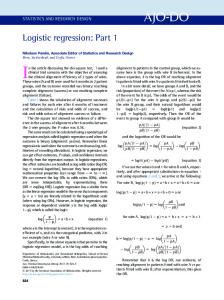
Logistic regression: Part 1. Nikolaos Pandis, Associate Editor of Statistics and Research Design. Bern, Switzerland, and Corfu, Greece. In the article discussing ...
The Logistic Regression Model (LRM) – Interpreting Parameters. [This handout
steals heavily from Linear probability, logit, and probit models, by John Aldrich.
Lipsitz, Laird and Harrington, 1991; Carey and Zeger, 1993). ... 2001), and mixed discrete and continuous (Dunson, 2000; Dunson, Chen and Harry, 2003).
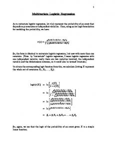
As in univariate logistic regression, let π(x) represent the probability of an ... So,
the form is identical to univariate logistic regression, but now with more than one.
A Logistic Regression Approach. P. K. Chauke1 and F. D. K. Anim. Department of Agricultural Economics, University of Venda,. Thohoyandou, 0950 South Africa.
1. Predictive Modeling. Logistic Regression. Logistic Regression. • Consider the
Multiple Linear Regression Model: i. 0. 1 i1. 2 i2 k ik i y = x x x β β β β ε. +. +. + +.
Predictive Modeling Logistic Regression
Logistic Regression • Consider the Multiple Linear Regression Model:
yi = β 0 + β1xi1 + β 2 xi2 +
+ βk xik + ε i
where the response variable y is dichotomous, taking on only one of two values: y =1 if a success =0 if a failure
1
Logistic Regression • The response variable, y, is really just a Bernoulli trial, with E(y) = π where π = probability of a success on any given trial • π can only take on values between 0 and 1
is not appropriate for a dichotomous response variable, since this model assumes π can take on any value, but in fact it can only take on values between 0 and 1.
2
Logistic Regression • When the response variable is dichotomous, a more appropriate linear model is the Logistic Regression Model:
π logit(π ) = log 1− π
= α + β1xi1 + β 2 xi2 +
+ βk xik
Logistic Regression • The ratio
π 1− π is called the odds, and is a function of the probability π
3
Logistic Regression • Consider the model with one predictor (k=1): Logit
Odds
π log 1− π
π 1− π
=α + βx α +β x
=e
α
=e
(e )
β x
Logistic Regression Odds
π 1− π
α
=e
(e )
β x
• Every one unit increase in x increases the odds by a factor of eβ
4
Logistic Regression x=1
x=2
x=3
π 1− π
π 1− π
π 1− π
( )
= eα e β
( )
= eα e β
3
= eα e β
( )
= eα e β
( )( eβ )
2
= eα e β
( )( eβ )( eβ )
Logistic Regression • Thus, eβ is the odds ratio, comparing the odds at x+1 with the odds at x • An odds ratio equal to 1 (i.e., eβ = 1) occurs when β = 0, which describes the situation where the predictor x has no association with the response y.
5
Logistic Regression • As with regular linear regression, we obtain a sample of n observations, with each observation measured on all k predictor variables and on the response variable. • We use these sample data to fit our model and estimate the parameters
Logistic Regression • Using the sample data, we obtain the model:
p log = a + bx 1-p for a single predictor
6
Logistic Regression • The estimate of π is
p=
ea+bx 1+ea+bx
Example: Coronary Heart Disease Odds
Log(Odds)
Age
Age Group (x)
CHD Present
N
p
p/(1-p)
log(p/(1-p)=a+bx
Predicted π-hat
25
1
1
10
0.10
0.09834
-2.31929
0.08954
30
2
2
15
0.13
0.17184
-1.76117
0.14664
35
3
3
12
0.25
0.30028
-1.20305
0.23093
40
4
5
15
0.33
0.52470
-0.64493
0.34413
45
5
6
13
0.46
0.91685
-0.08681
0.47831
50
6
5
8
0.63
1.60209
0.47131
0.61569
55
7
13
17
0.76
2.79947
1.02943
0.73681
60
8
8
10
0.80
4.89175
1.58755
0.83027
Exp(b) = 1.74738
b = 0.55812
(Multiplicative)
(Additive)
100
7
Example: Coronary Heart Disease Probability of Coronary Heart Disease 1.00
0.80 log(p/(1-p)) = -2.8774 + 0.5581 * X
Proportion
0.60
0.40 predicted observed 0.20
0.00 1
2
3
4
5
6
7
8
Age Group
Parameter Estimation • A 100(1-α)% Confidence Interval for β is:
βˆ ± zα / 2 × a.s.e. ( βˆ ) where zα/2 is a critical value from the standard normal distribution, and a.s.e. stands for the asymptotic standard error
8
Parameter Estimation • A 100(1-α)% Confidence Interval for the odds ratio eβ is:
e
βˆ ± zα / 2 ×a.s.e.( βˆ )
Hypothesis Testing H0: β = 0 H1: β ≠ 0 The test statistics for testing this hypothesis are χ2 statistics. There are 3 that are commonly used:
9
Hypothesis Testing 2
βˆ ∼ χ12 = a.s.e. βˆ
Wald Test
QW
Likelihood Ratio Test
QLR = −2 Lα − Lα ,β ∼ χ12
Score Test
QS ∼ χ12
( )
(
)
Goodness of Fit • Let m = # of levels of x (m=8 for CHD example) • Let ni = number of observations in the ith level of x • Let k = number of parameters (k=2 for CHD example) 2 XPearson
2 pi − πˆi ) ( 2 = ∑ ni ∼ χ m-k m
i=1
πˆi
m p 2 2 = 2 ∑ ni pi log i ∼ χ m-k XDeviance i=1 πˆi
10
Example: Coronary Heart Disease Odds
Log(Odds)
Age
Age Group (x)
CHD Present
N
p
p/(1-p)
log(p/(1-p)=a+bx
Predicted π-hat
25
1
1
10
0.10
0.09834
-2.31929
0.08954
30
2
2
15
0.13
0.17184
-1.76117
0.14664
35
3
3
12
0.25
0.30028
-1.20305
0.23093
40
4
5
15
0.33
0.52470
-0.64493
0.34413
45
5
6
13
0.46
0.91685
-0.08681
0.47831
50
6
5
8
0.63
1.60209
0.47131
0.61569
55
7
13
17
0.76
2.79947
1.02943
0.73681
60
8
8
10
0.80
4.89175
1.58755
0.83027
Exp(b) = 1.74738
b = 0.55812
(Multiplicative)
(Additive)
100
Logistic Regression Example Coronary Heart Disease vs. Age (first 25 observations, out of 100) Obs