Predictive Modeling of Pedestrian Motion Patterns with Bayesian ...

Predictive Modeling of Pedestrian Motion Patterns with Bayesian Nonparametrics Yu Fan Chen∗, Miao Liu†, Shih-Yuan Liu†, Justin Miller‡, Jonathan P. How§ Massachusetts Institute of Technology, Cambridge, MA, 02139, USA

For safe navigation in dynamic environments, an autonomous vehicle must be able to identify and predict the future behaviors of other mobile agents. A promising data-driven approach is to learn motion patterns from previous observations using Gaussian process (GP) regression, which are then used for online prediction. GP mixture models have been subsequently proposed for finding the number of motion patterns using GP likelihood as a similarity metric. However, this paper shows that using GP likelihood as a similarity metric can lead to non-intuitive clustering configurations – such as grouping trajectories with a small planar shift with respect to each other into different clusters – and thus produce poor prediction results. In this paper we develop a novel modeling framework, Dirichlet process active region (DPAR), that addresses the deficiencies of the previous GP-based approaches. In particular, with a discretized representation of the environment, we can explicitly account for planar shifts via a max pooling step, and reduce the computational complexity of the statistical inference procedure compared with the GP-based approaches. The proposed algorithm was applied on two real pedestrian trajectory datasets collected using a 3D Velodyne Lidar, and showed 15% improvement in prediction accuracy and 4.2 times reduction in computational time compared with a GP-based algorithm.

I.

Introduction

Advances in sensor technologies, computational capabilities, modeling and planning algorithms have led to increased levels of autonomy in mobile ground robots, such as indoor service robots1, 2 and self-driving cars.3, 4 Applications of such autonomous vehicles often require navigating in a stochastic world along with other dynamic agents, which include cars, cyclists, and pedestrians. To plan safe paths in such environments, an autonomous vehicle needs to be able to predict the future behaviors of the other agents. Kalman filters 5–8 are the most frequently used approaches for generating predictions by propagating system dynamics forward in time. However, applications of Kalman filters are often restricted to state predictions on a short time scale because they do not account for environmental structures and the agent’s underlying intentions (e.g. goal). This work focuses on predictive modeling on a longer time scale by learning the typical motion patterns from previously observed data. In particular, given observations of an agent’s trajectory, we want to find the most likely path that the agent may take in future. Predictive modeling of pedestrians presents additional challenges because (i) pedestrians’ intentions are often hidden (e.g. lack of dedicated turn signals) from the autonomous vehicle, (ii) pedestrians’ paths are less constrained by environmental structures (e.g. road lanes), and (iii) pedestrians are capable of sudden changes in their motion due to their less constrained dynamics. ∗ PhD

candidate, Department of Aeronautics and Astronautics, MIT, Cambridge, MA, 02139, Member AIAA Researcher, Laboratory of Information and Decision Systems, MIT, Cambridge, MA, 02139, Member AIAA ‡ PhD candidate, Department of Mechanical Engineering, MIT, Cambridge, MA, 02139 § Richard C. Maclaurin Professor of Aeronautics and Astronautics, MIT, Cambridge, MA, 02139, Associate Fellow AIAA

† Post-Doctoral

1 of 14 American Institute of Aeronautics and Astronautics

This paper presents an algorithm that learns motion patterns from previously observed trajectories, and uses these motion patterns to generate predictions of the pedestrians’ future behaviors. Cooperative models have been proposed for autonomous navigation in crowded indoor environments, such as shopping malls and cafeterias. For example, some researchers9, 10 model the interactions between the mobile robot and the pedestrians assuming that pedestrians follow certain collision avoidance rules. A data-driven approach11 models the joint motion pattern of the mobile robot and the pedestrians using Gaussian Processes. This class of models is more suitable for applications in which the mobile robot is operating in close proximity of the pedestrians at low speeds, where local interaction is more important than conforming to global environmental structures. In contrast, this paper focuses on pedestrian modeling in structured environments, such as at an intersection, where mobile vehicles are operating at higher speeds than pedestrians. To account for pedestrians’ intentions, Hidden Markov Models have been used for predictive modeling,12–14 typically with a pedestrian’s current position as the observed variable and the goal position as the hidden variable. The hidden states can either be specified by domain experts or learned through an Inverse Reinforcement Learning framework.15 Conditioned on the current position and the inferred goal position, predictions can be made by rolling the Markov model forward in time. Since Markov models are only conditioned on the last observed position, they can generate poor predictions if different motion patterns exhibit significantly overlapping segments.16 Moreover, pedestrian trajectories acquired from sensors mounted on mobile robots can be fragmented due to occlusion, for which the goal positions are difficult to identify. Gaussian Process (GP) based approaches17 overcome this problem by modeling motion patterns as velocity flow fields, thus avoiding the need to identify goal positions. Also, GPs are well-suited for applications with noisy measurements, such as for data collected on moving platforms. More importantly, predictions using a GP have a simple analytical form that can be easily integrated into a risk-aware path planner.18, 19 For persistent pedestrian behavior modeling in structured environments, a single GP model might not be sufficient to capture different types of motion patterns. Hence, a finite GP mixture model has been introduced in 20 to distinguish between multiple motion patterns. However, a finite mixture model is limited in flexibility because the number of motion patterns has to be specified a priori. Joseph et al.16 address this model uncertainty issue by developing Dirichlet process mixture of Gaussian processes (DPGPs), a Bayesian nonparametric model which learns the number of motion patterns and the shape of each motion pattern. Although GPs have been shown to be a good predictive tool,19 they can be a poor choice for clustering trajectories in a mixture model. In particular, this work shows that using GP likelihood as a similarity metric can lead to forming non-intuitive cluster configurations, and thereby produce poor prediction accuracy. The underlying issues are discussed in Section II.D. More importantly, combining DP and GP drastically increases the algorithm’s computational complexity. This paper proposes a novel model, Dirichlet process active region (DPAR), to address these problems. The main contributions of this paper are (i) showing that GP likelihood can be a poor similarity metric for clustering motion patterns, (ii) developing an active region (AR) model for motion pattern representation that results in better clustering performance than GP likelihood, (iii) developing the DPAR algorithm that runs 4-5 times faster than DPGP, and (iv) showing that DPAR produces higher prediction accuracy on datasets collected by a Velodyne Lidar mounted on a mobile robot.

II. II.A.

Preliminaries

Problem Statement

The trajectory of pedestrian i is denoted by ti , which is a sequence of li two dimensional position measurements {(x1 , y1 ), . . . , (xli , yli )} taken at a fixed time interval ∆t. The training set, D = {t1 , . . . , tS }, contains S trajectories with possibly different length. The objective of is defined as the following: given a training set D and tj−k:0 , which is the observation history of the past k time steps of pedestrian j who was not included in the training set, predict the most likely future path of pedestrian j, denoted by tj0:lj .

2 of 14 American Institute of Aeronautics and Astronautics

II.B.

Gaussian Process Motion Patterns

The Dirichlet process mixture of Gaussian Processes (DPGP) 16 is a mixture model of R motion patterns, where R is unknown a priori. A motion pattern, modeled by a pair of GPs, is a mapping from the 2D position space (x, y) to the 2D velocity space (vx , vy ), which can be more intuitively understood as a velocity flow field. ∆y In this work, velocities are computed using the finite difference approximation, that is, (vx , vy ) ≈ ( ∆x ∆t , ∆t ). A trajectory is assumed to be generated from one of the R motion patterns (i.e. following one streamline) with some added Gaussian measurement noise. Each motion pattern is modeled using a pair of single output GPs (for x and y velocities) with the squared exponential covariance function. Let cluster assignment zi ∈ {1, . . . , R} be an integer variable that specifies the motion pattern trajectory ti belongs to. A motion pattern bk can be learned by GP regression given a set of trajectories Dk = {tj |zj = k}, GP and a set of hyperparameters θpk . More precisely, the Gaussian process motion pattern is specified by a pair of mean and covariance functions, which are defined as follows, E [vx (x, y)] = µ1 (x, y), kp (x, y, x0 , y 0 ) = Ap exp

 −

E [vy (x, y)] = µ2 (x, y)

(y − y 0 )2 (x − x0 )2 − 2 2 2wp,x 2wp,y



(1)

+ Bp2 δ(x, y, x0 , y 0 )

(2)

where p ∈ {1, 2} corresponds to the x and y directions, respectively; δ(x, y, x0 , y 0 ) = 1 if x = x0 and y = y 0 and zero otherwise; wp,x and wp,y are the characteristic length-scales; and Bp is the variance of the measurement B noise. For predicting µp (x, y), the ratio App determines the relative influence of a measurement at position (x, y) with respect to nearby measurements. The tuple (Ap , Bp , wp,x , wp,y ) specifies the hyperparameters θpGP . For a pair of GPs trained with trajectory data Dk = {XDk , YDk , vx , vy }, the predictive distribution over (vx∗ , vy∗ ) for a new position (x∗ , y ∗ ) is given by µp (x∗ , y ∗ ) = µp (x∗ , y ∗ ) + Kp (x∗ , y ∗ , XDk , YDk )Kp (XDk , YDk , XDk , YDk )−1 (vp − µp ) σp2 (x∗ , y ∗ )

∗

∗

∗

∗

∗

∗

−1

= k(x , y , x , y ) − Kp (x , y , XDk , YDk )Kp (XDk , YDk , XDk , YDk )

(3) ∗

∗

Kp (XDk , YDk , x , y )

(4)

where vp = vx for p = 1 and vp = vy for p = 2, Kp (XDk , YDk , XDk , YDk ) is a training set covariance matrix and Kp (x∗ , y ∗ , XDk , YDk ) is a training-test set covariance vector. Readers are referred to16, 21 for GP regression details. Given a motion pattern bk characterized by data Dk , the likelihood of a trajectory ti with respect to this motion pattern is    
i i GP i GP p t |zi = k, Dk = LGP vx Dk , θ1k LGP vy Dk , θ2k , (5) where LGP denotes GP likelihood with  Y  l
i GP i LGP vx Dk , θ1k = N vxj ; µ1 (xij , yji ), σ12 (xij , yji ) ,

(6)

j=1

 where N denotes the Gaussian distribution. LGP

vyi

 Dk , θGP is constructed by replacing the hyperaram2k

eters corresponding to the y direction. II.C.

Clustering with a Dirichlet Process

The mixture components are modeled using a Dirichlet Process (DP) prior.22 In particular, DP specifies the probability of a data point i belonging to an existing cluster j, and to a new cluster K + 1, nij S−1+α α p(zi = K + 1|z−i , α) = S−1+α p(zi = j|z−i , α) =

j ∈ 1, . . . K

3 of 14 American Institute of Aeronautics and Astronautics

(7) (8)

P where nij = k,k6=i 1(zk = j) is the number of trajectories currently assigned to cluster j, z−i is the set of cluster assignments with zi removed, S is the number of trajectories in the dataset, and α is a concentration parameter that measures the variance of a DP.16 Combining Eq. (5) and Eq. (7), the probability of assigning a trajectory ti to an existing motion pattern bk , and to a new motion pattern bK+1 are

p zi = k|ti , α, bk = p ti |zi = k, bk p(zi = j|z−i , α) (9) Z

GP GP p zi = K + 1|ti , α, bk = p ti |zi = k, bk dθxk dθyk p(zi = K + 1|z−i , α). (10) The objective of the inference process is to find the number of clusters R, the cluster assignment zi for each of GP the S trajectories, and the hyperparameters θpk for each of the R behavior patterns. This learning process is typically carried out using Gibbs sampling for Eq. (10). In this work, the hyperparameter α is learned GP by sampling from an inverse gamma prior, and the hyperparameters θpk are determined by a grid-search procedure. II.D.

GP Likelihood as a Clustering Metric

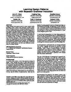
The DPGP algorithm works by first (i) grouping the set of trajectories into R clusters (finding zi ), and then (ii) fitting a pair of GPs to each cluster of trajectories. Implicit in the clustering step, GP likelihood as defined in Eq. (5) is used as a similarity metric. However, this section shows that using GP likelihood as a similarity metric can lead to poor clustering performance. In particular, the following paragraphs describe scenarios in which similar trajectories can be grouped into different clusters due to large differences in GP likelihood. While robust to measurement noise, GPs are not shift invariant. Since pedestrians often walk side-by-side, small planar shifts between pedestrian trajectories are common in real datasets. Fig. 1a illustrates an example of poor clustering performance using GP likelihood. In particular, given three trajectories (red, green, and black), we form a motion pattern (a pair of GPs) using the black trajectory, and then find the GP likelihood of the red and green trajectories with respect to this motion pattern. The mean (velocity flow field) and variance of the motion pattern formed by the black trajectory are illustrated in Fig. 1b and Fig. 1c, respectively. Due to a shift in the green curve with respect to the black curve, the observed velocities will be slightly different than the GP predictions everywhere along the curve, leading to a significant overall reduction in GP likelihood. More importantly, since variance is high in locations where a GP have not seen much data, such as inside the dotted blue box (see corresponding region in Fig. 1c), the red curve’s GP likelihood inside this region would not be low. As a consequence, compared to a slightly shifted green curve, the dissimilar but well aligned red curve can have higher likelihood with respect to the GP model formed by the black curve. This does not agree with the intuition that the green curve is more similar to the black curve than the red curve. Further, in real datasets, different people walking along the same curve can exhibit different speeds (ex. seniors often walk slower than young adults). Calculated based on the observed velocities, GP likelihood as a similarity metric often classifies trajectories traveling at different speeds into different clusters, even if these trajectories follow the same geometric curve. P Lastly, building a GP has O(L3k ) computational complexity,21 where Lk = {i|ti ∈Dk } li is total length of all trajectories assigned to the kth cluster. In this work, we implemented sparse GP as developed in,23 which has complexity O(|BV |2 Lk ), where |BV | is the number of basis vectors a . The Gibbs sampling inference procedure requires building GPs after every episode of resampling the cluster assignment zi , which is very time consuming.

III.

Dirichlet Process Active Region

This work is motivated by the insight that while GPs are good at modeling motion patterns for making predictions, GP likelihood can be a poor clustering metric and is computationally inefficient. We develop a The number of basis vectors presents a trade-off between representational power and computational complexity. In this work, we have chosen |BV | = 5.

4 of 14 American Institute of Aeronautics and Astronautics

6

0.4

4

2

2

0.4

0

0.6 .8 0

0

0.6

GP flow field training data

−4 −5

(a) three trajectories

0

0.2

0.2 0.4

−2

−2

−6

0.2

0.4 0.6

y (m)

y (m)

0.2

4

0.2

0. 0.6 4

0.8

6

−4

0.8

1

1

5

−6

−5

0

x (m)

x (m)

(b) GP flow field

(c) GP variance

5

Figure 1: An illustration of the deficiency of using GP likelihood for clustering. A small planar shift may lead to significant reduction in GP likelihood. Consider the three curves shown in subfigure (a). The red curve is well aligned with the black curve in the right half but the left half is dissimilar to the black curve. The green curve is a slightly shifted version of the black curve. Subfigure (b) and (c) show the resulting pair of GPs fitted to the black curve. Due to the alignment issue, the green curve can have a lower GP likelihood than the red curve, which implies that GP likelihood as a similarity measure specifies that the green curve is less similar to the black curve than the red curve.

Figure 2: Example of an active region motion pattern. The x-y plane is discretized into N × M squares, each with side length w. A darker color indicates a higher probability of a trajectory going through the grid location within a range of heading angle, which is shown in green.

a method in this section that has lower computational complexity and addresses the clustering problems described in Section II.D . III.A.

Active Region Motion Patterns

We develop an alternative motion pattern model that is computationally efficient to learn through posterior inference. We discretize the x-y plane into N × M blocks of side length w, as illustrated in Fig. 2. Each motion pattern bk is defined over the entire grid space, with each grid position associated with a Bernoulli random variable Akmn and a heading angle variable φkmn ∈ [0, 2π). Further, we parametrize each trajectory in the discretized space. For a trajectory ti in the dataset, we i compute the trajectory’s heading angle ψmn ∈ [0, 2π) within each grid position mn. If the trajectory does not go through a grid position, we assign the corresponding heading angle to be ∞. For each trajectory ti ik and each motion pattern bk , we associate an indicator variable Xmn to determine whether their heading

5 of 14 American Institute of Aeronautics and Astronautics

angles agree within an  threshold, such that  1 if ψ i − φk < , mn mn ik Xmn = 0 otherwise.

(11)

We call Akmn the activeness variable because it determines the probability that a trajectory goes through grid position mn; that is, a trajectory is more likely to go through an active grid, and is unlikely to go through an inactive grid. In particular, the likelihood of a trajectory ti belonging to a behavior pattern bk is
Y ik p ti |zi = k, bk = p(Xmn |Akmn ), (12) mn

where ik ik p(Xmn = 1|Akmn = 1) = pxa , p(Xmn = 0|Akmn = 1) = 1 − pxa ,

(13)

ik p(Xmn

(14)

=

1|Akmn

= 0) = pxn ,

ik p(Xmn

=

0|Akmn

= 0) = 1 − pxn .

In this work we choose pxa = 0.7 and pxn = 0.01, which is to enforce that it would be highly unlikely for a trajectory to go through an inactive grid position. Lastly, We place a uniform prior on the activeness variables, such that p(Akmn = 1) = p(Akmn = 0) = 0.5. III.B.

Posterior Inference

The objective of the inference process is to find the number of clusters R, the cluster assignment zi for each of the S trajectories, and the set of activeness variables Akmn and heading angle variables φkmn that determine each of the R motion patterns. The inference procedure is outlined in Algorithm 1. We initialize the number of clusters R and the cluster assignments zi in Lines 1 and 2. Then, we use Gibbs sampling for max iter iterations in Line 3. We found empirically that the set of clustering assignments would stabilize after approximately 100 iterations. Inside the main loop, we iterate between (i) learning the motion patterns given the set of assignment labels (Lines 5 to 8) and (ii) sampling the set of assignments given the motion patterns (Lines 10 to 13). Section III.B.1 and Section III.B.2 detail each of the two main steps. Lastly, we need to post-process the set of samples, such as removing burn-in samples and identifying the most likely sample in Line 14. III.B.1.

Update Motion Patterns

|=

Given the current set of cluster assignments zi , we first find the set of trajectories Dk = {ti |zi = k} belonging to the motion pattern bk . Note that conditional independence between grid position are assumed implicitly in the active region model defined in Eq. (14); more specifically Akmn Akrs ∀(m, n) 6= (r, s). And hence, Y p(bk |Dk ) = p(Akmn |Dk ). (15) mn

This assumption makes the model efficient to learn, since each term Akmn can be learned individually. Given the likelihood model defined in Eq. (14) and the prior p(Akmn = 1) = p(Akmn = 0) = 0.5, we obtain the posterior using Bayes’ rule, p(Akmn = 1|Dk ) =

p(Dk |Akmn

p(Dk |Akmn = 1)p(Akmn = 1) . = 1)p(Akmn = 1) + p(Dk |Akmn = 0)p(Akmn = 0)

Substituting Eq. (14) and let p(Akmn = 1) = pa , we obtain Q ik k 1)p(Akmn = 1) k i p(Xmn |Amn =Q Q p(Amn = 1|Dk ) = ik k k ik k k i p(Xmn |Amn = 1)p(Amn = 1) + i p(Xmn |Amn = 0)p(Amn = 0) sk nk −sk pa pxa (1 − pxa ) , = k k pa psxa (1 − pxa )nk −sk + (1 − pa )psxn (1 − pxn )nk −sk 6 of 14 American Institute of Aeronautics and Astronautics

(16)

(17a) (17b)

Algorithm 1: DPAR Inference 1 2 3 4 5 6 7 8 9 10 11 12

R ← N log N zi0 ← rand int(1, R) foreach s = 1: max iter do // update motion patterns given cluster assignments foreach motion pattern bk do Dk ← {ti |zis−1 = k} Akmn ← posteriorUpdate(Dk ) φkmn ← averageHeadingAngle(Dk ) // resample assignment labels given motion patterns foreach trajectory ti do l(k + 1) ← newClusterLikelihood(ti ) foreach motion pattern bk do l(k) ← existingClusterLikelihood(ti , bk ) zis ← sample(l)

13 14

zi ← postProcessing(zi1:max iter )

P ik P where sk = i Xmn is the number of trajectories going through the grid position mn, and nk = i I(zi = k) is the number trajectories assigned to the motion pattern bk . We note that p(Akmn = 1|Dk ) depends on the number of trajectories nk , which varies across different motion patterns. This would create an unintended aggregating effect for the clustering assignment step in Section III.B.2, which favors motion patterns with a larger number of trajectories. Thus, we choose to normalize the counts by a constant Nc , such that we k replace sk , nk with s¯k = sk /Nc , n¯k = nk /Nc , respectively, in Eq. (17). The heading angle ψmn is calculated by finding the average heading angle of the trajectories assigned to the motion pattern bk ,
k ψmn = mean φimn f or {i|zi = k}. (18) Additional care is needed when computing the mean of heading angles because of the angle wrapping issue, that is, φ = φ + 2π . In our implementation, we represent an angle φ as a tuple (cos φ, sin φ), and calculate the average by taking the mean of each component independently. III.B.2.

Update Cluster Assignments

Given a set of motion patterns {bk } built from the previous step, this subsection develops the likelihood equations for calculating Line 11 and Line 13 in Algorithm 1, which are used for sampling the cluster assignments. Combining Eq. (12) and Eq. (17), we obtain
X
p ti |zi = k, Dk−i = p ti |zi = k, bk p(bk |Dk−i ) (19a) bk

=

Y

X

ik p(Xmn |Akmn )p(Akmn |Dk−i ),

(19b)

mn Ak mn ∈{0,1}

where Dk−i is the set of trajectories Dk with element ti removed. To account for a planar shift, a problem described in Sec. II.D, we add a max pooling step in the likelihood calculation, X
Y ik p ti |zi = k, Dk−i = max p(Xmn |Aksr )p(Akst |Dk−i ) (20a) mn

s.t.

s,r

Ak sr ∈{0,1}

s ∈ {m − 1, m, m + 1}

(20b)

r ∈ {n − 1, n, n + 1},

(20c)

7 of 14 American Institute of Aeronautics and Astronautics

where the dummy variables s, r are introduced to account for a small planar shift by searching through a neighborhood centered at grid mn. In this work, we choose to search through all the immediately adjacent grid positions as defined in Eqs. (20b) and (20c) and find the neighbor sr that has the maximum likelihood value. We note that other neighborhood specifications can also be considered. Finally, we arrive at the expressions for sampling cluster assignments. The probability of assigning a trajectory ti to an existing motion pattern bk , and to a new motion pattern bK+1 are

p zi = k|ti , α, Dk−i = p ti |zi = k, Dk−i p(zi = j|z−i , α) (21) Z

p zi = K + 1|ti , α, Dk−i = p ti |zi = k, bk dbk p(zi = K + 1|z−i , α), (22) where the last term is defined in Eq. (8). III.C.

Active Region Likelihood as a Clustering Metric

The active region likelihood defined in Eq. (14) was used as a similarity metric for sampling cluster assignment labels in Eq. (22). By adding a max pooling step in Eq. (20), we see that a small planar shift would not affect the computed likelihood. This leads to a natural interpretation of the w hyperparameter as a typical length scale of a dataset, such as the width of a sidewalk. Further, the active region model uses the heading angles, rather than the velocities along each trajectory for calculating likelihood. Thus, trajectories traversing at different speeds along the same curves would be classified into the same cluster. This approach addresses the issues described in Section II.D. In P addition, the computational complexity of building an active region motion pattern bk is O(|Lk |) where Lk = {i|ti ∈Dk } li is the total length of all trajectories assigned to the kth cluster. The posterior inference ik procedure is efficient because it only requires finding Xmn by element-wise comparison, and computing the ik statistics of nk and sk by summing the corresponding terms Xmn . The output of Algorithm 1 is a set of clustering assignments zi , which are used to form GPs as described in16 for online prediction.

IV.

Results

Pedestrian trajectories are extracted from streams of 3D point cloud data collected with a Velodyne Lidar. A point cloud containing the scene with no pedestrian is set as the background key frame. We remove the background from each incoming frame using the octree implementation in the pcl libraryb , and obstain a foreground point cloud containing only the mobile agents. Points in the foreground point cloud are clustered using the dynamic means algorithm,24 which tracks moving clusters. A pedestrian trajectory corresponds to the path traced out by the centroid of a cluster. We apply the DPAR algorithm on two pedestrian trajectory datasets; the first dataset containing 143 trajectories is collected at the intersection of two corridors, and the second dataset containing 96 trajectories is collected in the lobby area of a building. Each trajectory is a timestamped sequence of position measurements down-sampled to a frequency of 2Hz. The average length of each trajectory is about 12 meters. We hold 75% of the trajectories in a dataset as the training set and the remaining 25% as the test set. We ran DPAR on the training set to construct R motion patterns, which in turn, are used to make predictions for trajectories in the test set. The datasets are shown in Fig. 3. IV.A.

Prediction Accuracy

We ran the DPAR algorithm as described in Algorithm 1 on each dataset to find cluster assignments, zi , for trajectories in the training set. The clustering result of DPAR on dataset I is shown in Fig. 7, which corresponds well to how a person would cluster the data. For each cluster, we form a GP motion pattern as described in Section II.B. For each trajectory in the test set, we make predictions based on the observed b See

http://pointclouds.org/documentation for more information

8 of 14 American Institute of Aeronautics and Astronautics

15 15 10

y (m)

y (m)

10 5

5

0 0 −5 −5

−10 −15

−10

−5

0 x (m)

5

10

15

−15

(a) dataset I - training set with 108 trajectories

−10

−5

0 x (m)

5

10

(b) dataset II - training set with 72 trajectories

15

10

10 y (m)

y (m)

5

5

0 0 −5 −5 −10

−5

0 x (m)

5

10

−15

(c) dataset I - test set with 35 trajectories

−10

−5

0 x (m)

5

10

(d) dataset II - test set with 24 trajectories

Figure 3: Two pedestrian trajectory datasets. Dataset I is collected at the intersections of two corridors, and dataset II is collected in the lobby area of a building. The latter environment has fewer structures that would restrict a pedestrian’s motion . Each trajectory is plotted in blue. The asterisk marks the starting point of a trajectory. Motion patterns are learned from the training set and evaluated on the test set.

trajectory segment. In particular, suppose a trajectory contains a sequence of l position measurements at every 0.5 seconds. We first partition a segment of length two, containing measurements from time 0 – 0.5 seconds. Given this segment, we find the GP motion pattern that most likely generated this segment (Eq. (5)), and we make a prediction for 5 seconds into the future using this GP motion pattern. The predicted trajectory is compared with the actual trajectory from 0.5 – 5.5 seconds. The prediction step is illustrated in Fig. 4. We repeat this process for each time step, making predictions by conditioning on the observed segment of increasing length. Figure 5 shows that DPAR attains better prediction accuracy than DPGP. More precisely, DPAR attains 22% and 5% error reduction compared to DPGP on dataset I and II, respectively. We distinguish dataset I from dataset II by noting that the latter environment has fewer environmental structures that would restrict a pedestrian’s motion. Thus, most trajectories from dataset II are smooth curves connecting the start and end positions; and there is little overlap between trajectories with different start and end positions. In short, dataset II does not exhibit the scenarios described in Section II.D and we expect both algorithms to show similar prediction accuracy on dataset II. Empirically, we see a smaller improvement of DPAR over DPGP for dataset II. Furthermore, we clustered dataset I by hand as ground truth. Fig. 6 shows that DPAR achieves similar prediction accuracy compared to using the hand-labeled clustering assignments.

9 of 14 American Institute of Aeronautics and Astronautics

4 start prediction

y (m)

2 0 −2

predictive flow field training data predicted traj observed traj initial position

−4 −6 0

5 x (m)

10

Figure 4: Prediction using a pair of GPs. Given a pedestrian’s path (from the initial position marked with the magenta asterisk to the current measurement marked with the green circle), we first find the pair of GPs (blue flow field) that most likely generated this path. The pair of GPs are learned from the set of trajectories (shown in red) that are assigned to this motion pattern. From the current measurement, we propagate the GP for 5 seconds into the future, hence generating a predicted trajectory marked in green. We evaluate the accuracy of the predicted trajectory by comparing with the observed trajectory (black line from the green circle to the end). In particular, we calculate the 2 norm distance between the two lines.

IV.B.

Computational Time

The algorithms are run on a computer with an Intel i7-4510U CPU and 16GB of memory. Recall computational complexity for sparse-DPGP and DPAR are O(|BV |2 L) and O(L), respectively. Empirical evaluation shows that DPAR is about 4.3 times faster than DPGP, as shown in Table 1. Table 1: Average and variance of computational time (secs). This table compares the computational time of DPGP and DPAR running 200 Gibbs sampling steps on the two datasets shown in Fig. 3. Dataset I Dataset II

V.

DPAR

sparse-DPGP

92.3 (12.1) 189.6 (21.0)

377.3 (56.3) 920.1 (106.0)

Conclusion

This paper has developed a data-driven approach for learning a mobile agent’s motion patterns from past observations, which are subsequently used for online trajectory predictions. We examined why previous GP-based mixture models can sometimes produce poor prediction results by providing examples to show that while Gaussian process (GP) is a flexible tool for modeling motion patterns, GP likelihood is not a good

10 of 14 American Institute of Aeronautics and Astronautics

3.5

4

2.5

RMS error (m)

RMS error (m)

3

5 DPAR DPGP

2 1.5 1

DPAR DPGP

3 2 1

0.5 0

0

0 2 4 6 8 time since started tracking a pedestrian (s)

0 2 4 6 time since started tracking a pedestrian (s)

(a) dataset I - RMS prediction error

(b) dataset II - RMS prediction error

Figure 5: DPGP vs. DPAR RMS prediction error. The x-axis shows for how much time has a pedestrian been observed. At each time step, we make a prediction for 5 seconds into the future as described in Fig. 4, and calculated the RMS error between the predicted path and actual path. This figure shows the average RMS prediction error for all trajectories in the training set. The solid lines and the shaded region show the median and the 25-75 percentile prediction error, respectively. In dataset I, DPAR achieves 22% error reduction compared to DPGP. In dataset II, DPAR is marginally better than DPGP. 2.5 DPAR hand labeled

RMS error (m)

2

1.5

1

0.5

0

0

2 4 6 time since started tracking a pedestrian (s)

8

Figure 6: DPAR vs. hand-labeled RMS prediction error on dataset I. As for ground truth, we clustered dataset I by hand and then fitted a pair of GPs to each cluster. We evaluated the performance of the hand-labeled results against that of DPAR. On dataset I, DPAR yielded comparable performance to that of a hand-labeled clustering assignment.

11 of 14 American Institute of Aeronautics and Astronautics

10 5 0 −5 −10

0

10

Figure 7: DPAR finds 16 clusters from dataset I (Fig. 3a). All sub-figures have the same axis as the top left sub-figure. Each sub-figure plots the trajectories assigned to one of the clusters.

12 of 14 American Institute of Aeronautics and Astronautics

similarity measure for trajectory clustering. The proposed algorithm, Dirichlet process active region (DPAR), addresses the deficiencies of the GP-based approaches and achieves better computational tractability. The proposed algorithm is applied on two real pedestrian datasets and showed improvement in prediction accuracy and significant reduction in computational time compared to a GP-based algorithm. In future studies, we will integrate the proposed algorithm with a risk aware path planner for improving the safety of autonomous navigation through urban environments.

Acknowledgments This work is supported by Ford Motor Company.

References 1 Bilge Mutlu and Jodi Forlizzi. Robots in organizations: the role of workflow, social, and environmental factors in human-robot interaction. In Human-Robot Interaction (HRI), 2008 3rd ACM/IEEE International Conference on, pages 287–294. IEEE, 2008. 2 Takayuki Kanda, Masahiro Shiomi, Zenta Miyashita, Hiroshi Ishiguro, and Norihiro Hagita. A communication robot in a shopping mall. Robotics, IEEE Transactions on, 26(5):897–913, 2010. 3 Sebastian Thrun, Mike Montemerlo, Hendrik Dahlkamp, David Stavens, Andrei Aron, James Diebel, Philip Fong, John Gale, Morgan Halpenny, Gabriel Hoffmann, et al. Stanley: The robot that won the darpa grand challenge. Journal of field Robotics, 23(9):661–692, 2006. 4 Julius Ziegler, Philipp Bender, Markus Schreiber, Henning Lategahn, Tobias Strauss, Christoph Stiller, Thao Dang, Uwe Franke, Nils Appenrodt, C Keller, et al. Making bertha drive? an autonomous journey on a historic route. Intelligent Transportation Systems Magazine, IEEE, 6(2):8–20, 2014. 5 Nicolas Schneider and Dariu M Gavrila. Pedestrian path prediction with recursive bayesian filters: A comparative study. In Pattern Recognition, pages 174–183. Springer, 2013. 6 M Bertozzi, A Broggi, A Fascioli, A Tibaldi, R Chapuis, and F Chausse. Pedestrian localization and tracking system with kalman filtering. In Intelligent Vehicles Symposium, 2004 IEEE, pages 584–589. IEEE, 2004. 7 Raj Madhavan and Craig I Schlenoff. Moving object prediction for off-road autonomous navigation. In AeroSense 2003, pages 134–145. International Society for Optics and Photonics, 2003. 8 Uwe Franke, Clemens Rabe, Hern´ an Badino, and Stefan Gehrig. 6d-vision: Fusion of stereo and motion for robust environment perception. In Pattern Recognition, pages 216–223. Springer, 2005. 9 Sungjoon Choi, Eunwoo Kim, and Songhwai Oh. Real-time navigation in crowded dynamic environments using gaussian process motion control. In Robotics and Automation (ICRA), 2014 IEEE International Conference on, pages 3221–3226. IEEE, 2014. 10 Stephen J Guy, Jatin Chhugani, Changkyu Kim, Nadathur Satish, Ming Lin, Dinesh Manocha, and Pradeep Dubey. Clearpath: highly parallel collision avoidance for multi-agent simulation. In Proceedings of the 2009 ACM SIGGRAPH/Eurographics Symposium on Computer Animation, pages 177–187. ACM, 2009. 11 Peter Trautman, Jeremy Ma, Richard M Murray, and Andreas Krause. Robot navigation in dense human crowds: the case for cooperation. In Robotics and Automation (ICRA), 2013 IEEE International Conference on, pages 2153–2160. IEEE, 2013. 12 Dimitrios Makris and Tim Ellis. Spatial and probabilistic modelling of pedestrian behaviour. In BMVC, pages 1–10. Citeseer, 2002. 13 Allison Bruce and Geoffrey Gordon. Better motion prediction for people-tracking. In Proc. of the Int. Conf. on Robotics & Automation (ICRA), Barcelona, Spain, 2004. 14 Dizan Vasquez, Thierry Fraichard, and Christian Laugier. Incremental learning of statistical motion patterns with growing hidden markov models. Intelligent Transportation Systems, IEEE Transactions on, 10(3):403–416, 2009. 15 Bernard Michini, Mark Cutler, and Jonathan P How. Scalable reward learning from demonstration. In Robotics and Automation (ICRA), 2013 IEEE International Conference on, pages 303–308. IEEE, 2013. 16 Joshua Joseph, Finale Doshi-Velez, Albert S Huang, and Nicholas Roy. A bayesian nonparametric approach to modeling motion patterns. Autonomous Robots, 31(4):383–400, 2011. 17 David Ellis, Eric Sommerlade, and Ian Reid. Modelling pedestrian trajectory patterns with gaussian processes. In Computer Vision Workshops (ICCV Workshops), 2009 IEEE 12th International Conference on, pages 1229–1234. IEEE, 2009. 18 Georges S Aoude, Brandon D Luders, Joshua M Joseph, Nicholas Roy, and Jonathan P How. Probabilistically safe motion planning to avoid dynamic obstacles with uncertain motion patterns. Autonomous Robots, 35(1):51–76, 2013. 19 Sarah Ferguson, Brandon Luders, Robert C Grande, and Jonathan P How. Real-time predictive modeling and robust avoidance of pedestrians with uncertain, changing intentions. arXiv preprint arXiv:1405.5581, 2014. 20 Kihwan Kim, Dongryeol Lee, and Irfan Essa. Gaussian process regression flow for analysis of motion trajectories. In Computer Vision (ICCV), 2011 IEEE International Conference on, pages 1164–1171. IEEE, 2011. 21 Carl Edward Rasmussen. Gaussian processes for machine learning. 2006.

13 of 14 American Institute of Aeronautics and Astronautics

22 Samuel J Gershman and David M Blei. A tutorial on bayesian nonparametric models. Journal of Mathematical Psychology, 56(1):1–12, 2012. 23 Lehel Csat´ o and Manfred Opper. Sparse on-line gaussian processes. Neural computation, 14(3):641–668, 2002. 24 Trevor Campbell, Miao Liu, Brian Kulis, Jonathan P. How, and Lawrence Carin. Dynamic clustering via asymptotics of the dependent dirichlet process mixture. In Advances in Neural Information Processing Systems 26, 2013.

14 of 14 American Institute of Aeronautics and Astronautics