Dec 1, 2008 - difficulty in a full simulation is the simultaneous solution of the ..... electrostatic forces present for sorbents with an ionic structure such as zeolites. ... Finally, due to the lack of strong polar bonds, the bond strength is lower than.
PREDICTIVE SIMULATION OF GAS ADSORPTION IN FIXED-BEDS AND LIMITATIONS DUE TO THE ILL-POSED DANCKWERTS BOUNDARY CONDITION
by
JAMES CLINTON KNOX
A DISSERTATION
Submitted in partial fulfillment of the requirements For the degree of Doctor of Philosophy in The Department of Mechanical and Aerospace Engineering to The School of Graduate Studies of The University of Alabama in Huntsville
HUNTSVILLE, ALABAMA 2016
TABLE OF CONTENTS Page List of Figures .................................................................................................................... ix List of Tables ................................................................................................................... xvi List of Acronyms ........................................................................................................... xviii Nomenclature ....................................................................................................................xx Chapter I ..............................................................................................................................1 1.
INTRODUCTION ...................................................................................................1
Chapter II .............................................................................................................................7 2.
ADSORBENTS AND GAS SEPARATION PROCESSES ....................................7 2.1 Gas Separations in Current Use ...................................................................7 2.1.1 Criteria for Commercial Use of Gas Adsorption .............................8 2.1.2 Applications of Gas Adsorption for Atmospheric Control in Habitable Volumes ....................................................................10 2.1.3 Adsorbents in Current Use .............................................................12 2.1.4 Equilibrium Capacity Isotherms ....................................................21 2.1.5 Mass Transfer Mechanisms in Fixed-Beds ....................................23 2.1.6 Linear Driving Force Model ..........................................................27 2.2 Emerging Applications of Gas Separations ...............................................28 2.2.1 Emerging Applications in the Chemical Processing Industry .......28 2.2.2 Efforts to Develop Affordable Flue Gas CO2 Capture Systems ....29 2.2.3 Spacecraft Life Support Needs for Reduced Mass/Power/ Volume Systems ............................................................................32 2.3 Virtual Design of Gas Separation Systems ................................................34 2.4 Literature Review of Adsorption Models ..................................................37 2.4.1 Applications ...................................................................................37 2.4.2 Experimental System .....................................................................37 2.4.3 Spatial Dimensions ........................................................................38 2.4.4 Tube Inner Diameter/Particle Diameter .........................................38 2.4.5 Gas to Particle Rate Expression .....................................................39 2.4.6 Method to Determine Gas to Particle Rate ....................................40 2.4.7 Axial Dispersion ............................................................................40 2.4.8 Internal Profile Shown? .................................................................41
Chapter III ..........................................................................................................................42
vi
3.
EXPERIMENTAL .................................................................................................42 3.1 Objective ....................................................................................................43 3.2 Test Apparatus ...........................................................................................43 3.2.1 Packed Column ..............................................................................43 3.2.2 Sensors ...........................................................................................46 3.2.3 Data Acquisition ............................................................................48 3.2.4 Support Equipment ........................................................................48 3.3 Procedures ..................................................................................................49 3.3.1 Adsorption Procedure ....................................................................49 3.3.2 Desorption Procedure.....................................................................50 3.4 Analysis to Determine Experimental Uncertainty .....................................52 3.4.1 Carbon Dioxide Breakthrough Data Reduction Procedure ............52 3.4.2 Carbon Dioxide Breakthrough Test Uncertainty Analysis ............55 3.4.3 Humidity Breakthrough Test Uncertainty Analysis ......................61
Chapter IV..........................................................................................................................66 4.
LIMITATIONS OF BREAKTHROUGH CURVE ANALYSIS IN FIXED-BED ADSORPTION ...........................................................................66 4.1 Introduction ................................................................................................67 4.2 Mathematical Model ..................................................................................70 4.2.1 Gas-Phase Mass Balance ...............................................................70 4.2.2 Adsorbed-Phase Mass Balance ......................................................71 4.2.3 Energy Balance ..............................................................................72 4.2.4 Equilibrium Adsorption Isotherms ................................................74 4.2.5 Axial Dispersion Coefficient .........................................................76 4.2.6 Gas-Phase Properties: Heat Transfer .............................................77 4.2.7 Correlations for Heat Transfer Coefficients ..................................77 4.2.8 Effective Thermal Conductivity ....................................................78 4.3 Numerical Approach and Validation .........................................................79 4.3.1 Code Validation .............................................................................80 4.4 Sensitivity of Simulation to Heat Transfer Correlations............................82 4.4.1 Sensitivity of Simulation Results to Heat Transfer Correlations ...83 4.4.2 Sensitivity of Simulation Results to Use of Constant Heat Transfer Coefficients .............................................................91 4.5 Results and Discussion ..............................................................................92 4.5.1 Thermal Characterization Tests and Fitting of Heat Transfer Parameter .......................................................................................93 4.5.2 Experimental Breakthrough Tests for CO2 and H2O Vapor on Zeolite 5A .................................................................................95 4.5.3 Empirical Determination of the LDF Mass Transfer Coefficient kn .................................................................................99 4.5.4 Non-Plug Flow Axial Dispersion Coefficient Determination on Zeolite 5A ...............................................................................107 4.6. Modeling Conclusions .............................................................................116 4.7 Ramifications for Large and Small Diameter Fixed-beds .......................119
vii
Chapter V .........................................................................................................................123 5.
MAPPING THE SENSITIVITY OF SORBATE/SORBENT SYSTEMS TO THE AXIAL DISPERSION COEFFICIENT AND LDF COEFFICIENT...123 5.1 Introduction ..............................................................................................123 5.2 Identifying the Non-physical Threshold for CO2 on Zeolite 5A .............123 5.3 Identifying the Non-physical Threshold for H2O on Zeolite 5A .............131 5.4 Identifying the Non-physical Threshold for CO2 and H2O on Zeolite 13X .........................................................................................135 5.5 Generalization to Other Sorbent/Sorbate Systems ...................................138 5.6 Conclusions for Parameter Mapping .......................................................142
Chapter VI ........................................................................................................................144 6.
CONCLUSIONS..................................................................................................144
APPENDIX A: LITERATURE REVIEW OF FIXED BED GAS ADSORPTION MODELS UNCERTAINTY ANALYSIS ...........................................149 APPENDIX B: UNCERTAINTY ANALYSIS ..............................................................152 APPENDIX C: VIRTUAL ADSORPTION TEST SUITE ............................................171 APPENDIX D: VALIDATION OF DIFFUSION AND VISCOSITY CORRELATIONS ................................................................................246 APPENDIX E: VALIDATION OF VIRTUAL ADSORPTION TEST SUITE ............268 APPENDIX F: VARIANCE IN CORRELATIONS DUE TO TEMPERATURE CHANGES ............................................................................................284 REFERENCES ................................................................................................................309
viii
LIST OF FIGURES Figure
Page
2.1
Four-bed molecular sieve CO2 removal system schematic (Knox, 2000) ............12
2.2
SEM images of silica gel used in the ISS CDRA. Note the circle identifying one of the primary particles in the 15kx view (15kx image from http://www.grace.com/EngineeringMaterialScience/SilicaGel/ SilicaGelStructure.aspx), other images from Radenburg, 2013) ...........................15
2.3
(a) Pelletized zeolite pellets, (b) crystals, and (c) framework structure http://www.grace.com/engineeredmaterials/productsandapplications/ InsulatingGlass/SieveBeads/Grades.aspx) ............................................................19
2.4
SEM images of pelletized zeolite 5A used in the ISS CDRA. Individual zeolite crystals are evident in the 1kx views (Radenburg, 2013) .........................20
2.5
Equilibrium capacity isotherms for CO2 on zeolite 5A, where data points represent test data and the lines represent the Toth fit to the data (Wang and LeVan, 2009) ........................................................................................................21
2.6
Isotherm types I through V, where pi is sorbate partial pressure, ni is sorbent loading, and is the sorbate saturated pressure (Brunauer et al., 1940) ............23
2.7
Packed (or fixed) bed of zeolite 13X beads. Photo taken by author .....................24
2.8
Depiction of fixed-bed and zeolite mass transfer mechanisms (Shareeyan et al., 2014) ........................................................................................25
2.9
Key technologies and associated research focus for post-combustion capture (U.S. DOE, 2013) .....................................................................................31
2.10
Integrated optimization approach flowchart (Knox, 2015) ...................................35
3.1
(a) Breakthrough test apparatus of Knox (1992b) and (b) cross-sectional view of typical sampling location .........................................................................44
3.2
Fixed adsorbent bed cutaway (Knox, 1992b) .......................................................45
3.3
MSMBT adsorption schematic (Knox, 1992b) .....................................................47
3.4
MSMBT desorption test apparatus (Knox, 1992b) ...............................................50
3.5
Typical uncertainty distribution for a CO2 concentration measurement ...............58 ix
3.6
Temporal variation in CO2 breakthrough test due to uncertainty in flow meter: Variation in concentration (left) and temperature (right) at midpoint (top) and exit (bottom) ...................................................................................................60
3.7
Temporal variation in water dioxide breakthrough test due to uncertainty in flow meter: Variation in concentration (left) and temperature (right) at midpoint (top) and exit (bottom) .......................................................................65
4.1
Equilibrium adsorption isotherms for CO2 (top) and H2O vapor (bottom) on zeolite 5A at temperatures from 0°C to 100°C as indicated. Symbols represent experimental data; Toth isotherm fits are shown as lines (Wang and LeVan, 2009) ..................................................................................................75
4.2a
Thermal characterization simulation results with varying sorbent to gas heat transfer (hs) coefficient of 68.2 (dotted line) and 93.6 (dashed line) W・m-2・K-1. Left side plots show the full simulation, while right plots are zoomed in to observe differences in the simulation results .............................88
4.2b
Thermal characterization simulation results with varying effective axial transfer conductance (keff) of 0.453 (dotted line) and 2.27 (dashed line) W・m-2・K-1 ..........................................................................................................88
4.2c
Thermal characterization simulation results with varying gas to internal column wall heat transfer coefficient (hi) of 14.3 (dotted line) and 15.7 (dashed line) W・m-2・K-1 ....................................................................................88
4.3
Sum of square error vs. ho for the thermal characterization simulation. Blue circles: SSE for values from thermal correlations selected for use in the work: hs = 92.2 W m-2 K-1; keff = 0.793 W m K-1; and hi = 13.7 W m-2 K-1. Black squares: SSE for values from worst-case thermal correlations: hs = 68.2 W m-2 K-1; keff = 2.74 W m K-1; and hi = 14.3 W m-2 K-1 ................89
4.4
Sum of square errors vs. kn for the CO2 breakthrough simulation. Blue circles: SSE for values from thermal correlations selected for use in the work: hs = 104 W m-2 K 1; keff = 0.653 W m K-1; hi = 12.5 W m-2 K-1; and ho = 1.69 W m-2 K-1. Black squares: SSE for values from worst-case thermal correlations: hs = 85.8 W m-2 K-1; keff = 2.27 W m K-1; hi = 12.6 W m-2 K-1; and ho = 1.66 W m-2 K-1. Callouts show that the minimum SSE occurs for a value of kn = 0.24 s-1 ...........................................91
4.5
Temperature history data for the thermal characterization test with N2 on zeolite 5A at three centerline locations in the bed (circles: 2.5%, squares: 50%, and diamonds: 97.5%). Left Panel: Experimental data with error bars showing experimental uncertainty. Right Panel: Experimental data with corresponding x
predictions from the model with the heat transfer coefficient from the column wall to the surroundings ho = 1.69 Wm-1K-1 ......................................95 4.6a
Experimental gas-phase concentration profile history breakthrough curves for CO2 on zeolite 5A at three centerline locations in the bed (circles: 2.5%, squares: 50%, and diamonds: 97.5%), and just outside the bed (triangles) ..........96
4.6b
Corresponding experimental temperature profile histories for H2O vapor on zeolite 5A at three centerline locations in the bed. Error bars show experimental uncertainty .......................................................................................96
4.7
Experimental gas-phase concentration profile history breakthrough curves for CO2 (dotted lines) and H2O vapor (solid lines) on zeolite 5A at two centerline locations in the bed (squares: 50%, and diamonds: 97.5%), and just outside the bed (triangles) plotted against dimensionless time defined relative to the respective breakthrough time for each adsorbate for the breakthrough curve measured just outside the bed, i.e., tBT ....................................................................................................................98
4.8
Fits of the 1-D axial dispersed plug flow model to the 97.5% location (diamonds) experimental centerline gas-phase concentration breakthrough curves for CO2 (left) and H2O vapor (right) on zeolite 5A, and corresponding predictions from the model of the 2.5% (circles) and 50% (squares) locations. Diamonds: experimental data; dashed lines: simulations with the Edwards and Richardson correlation for axial dispersion (Equation (4.10a)) and corresponding kn values (Table 4.7); dotted lines: simulations with the Wakao and Funazkri correlation for axial dispersion (Equation (4.10b)) and corresponding kn values (Table 4.7d). The saturation term in the CO2-zeolite 5A isotherm was increased by 15%. The saturation term in the H2O vapor-zeolite 5A isotherm was decreased by 3%. The void fraction was reduced to 0.33 based on the Cheng distribution (Cheng et al., 1991) with C = 1.4 and N = 5, as recommended by Nield and Bejan (1992) .....102
4.9a
CO2 on zeolite 5A: Predictions from the model (lines) shown in Figure 4.8 of the 2.5% (circles), 50% (squares), and 97.5% location (diamonds) experimental center line gas-phase concentration breakthrough curves (left), but now using the reported saturation term for the CO2-zeolite 5A isotherm (no adjustment), a void fraction of 0.33, the Wakao and Funazkri correlation (Equation (4.10a)) for axial dispersion and LDF kn = 0.0023 s-1. The experimental outside the bed (triangles) breakthrough curve is shown for comparison. Predictions from the model (lines) of the 2.5% location (circles), 50% location (squares), and 97.5% location (diamonds) experimental center line temperature profile histories (right) ....................................................................104
4.9b
H2O on zeolite 5A: (a) Predictions from the model (lines) shown in Figure 4.5 of the 2.5% location (circles), 50% location (squares), and 97.5% location (diamonds) experimental center line gas-phase concentration breakthrough
xi
curves, but now using the reported saturation term for the H2O-zeolite 5A isotherm (no adjustment), a void fraction of 0.33, the Wakao and Funazkri correlation (Equation 4.10b) for axial dispersion and LDF kn = 0.0008 s-1. The experimental outside the bed (triangles) breakthrough curve is shown for comparison. Predictions from the model (lines) of the 2.5% location (circles), 50% location (squares), and 97.5% location (diamonds) experimental center line temperature profile histories. (b) H2O on zeolite 5A (bottom panels): same as (a), but now with LDF kn adjusted to kn = 0.0002 s-1 to match the slope of the experimental outside the bed (triangles) breakthrough curve .............................105 4.10
CO2 on zeolite 5A: Fit of the 1-D axial dispersed plug flow model to the outside bed (triangles) experimental breakthrough curve using a value of DL 7 times greater than that from the Wakao and Funazkri correlation and the fitted LDF kn = 0.0023 s-1 (left panel). The reported saturation term for the CO2-zeolite 5A isotherm was used, along with the reported void fraction of 0.35. Predictions from the model (lines) of the gas-phase concentration breakthrough curves at 0, 4, 8, 12, …, 92, 96, and 100% locations in the bed are also shown in the left panel, along with the 2.5% (circles), 50% (squares), and 97.5% location (diamonds) experimental center line gas-phase concentration breakthrough curves (left panel). The corresponding derivative (or slope) of the predicted gas-phase concentration breakthrough curves in the bed are shown in the middle panel. Predictions from the model (lines) of the 2.5% (circles), 50% (squares), and 97.5% location (diamonds) experimental center line temperature profile histories are shown in the right panel .................................................................................................109
4.11
H2O vapor on zeolite 5A: Predictions from the 1-D axial dispersed plug flow model of the outside the bed (triangles) experimental breakthrough curve when varying the value of DL. DL = 10 (dotted lines), 30 (dashed lines), 50 (solid lines), and 70 (dash-dot lines) times greater than Wakao and Funazkri correlation with the LDF kn = 0.00083 s-1 (left panel). The reported saturation term for the H2Ozeolite 5A isotherm was used, along with the reported void fraction of 0.35. The corresponding predictions from the model (lines) of the 2.5% (circles), 50% (squares), and 97.5% location (diamonds) experimental center line temperature profile histories are shown in the right panel ......................................................110
4.12
H2O vapor on zeolite 5A: Predictions from the model (lines) shown in Figure 4.11 of the gas-phase concentration breakthrough curves at 0, 4, 8, 12, …, 92, 96, and 100% locations in the bed (left panels). The 2.5% (circles), 50% (squares), and 97.5% location (diamonds) experimental centerline gas-phase concentration breakthrough curves are also shown for comparison in the left panels. The corresponding derivatives (or slopes) of the gas-phase concentration breakthrough curves in the bed are shown in the right panels. (a) DL = Wakao-Funazkri correlation, (b) DL = 7, (c) 30, and (d) 50 times greater than Wakao and Funazkri correlation .....................................................114
xii
4.13
Carbon dioxide removal system sorbent bed. Heater sheets are brown in color and run vertically. Folded aluminum channel fins (gray) distribute heat from the heater sheets. The sorbent material (light tan) has been partially loaded to the outside and lower portion of the bed (Coker et al., 2015) ..................................121
5.1
Carbon dioxide on zeolite 5A: Predictions from the model (lines) of the gas-phase concentration breakthrough curves at 0, 4, 8, 12… 92, 96, and 100% locations in the bed (left panels). The 2.5% (circles), 50% (squares), and 97.5% location (diamonds) experimental centerline gas-phase concentration breakthrough curves are also shown for comparison in the left panels. The corresponding derivatives (or slopes) of the gas-phase concentration breakthrough curves in the bed are shown in the right panels. (a) DL = Wakao-Funazkri correlation, (b) DL = 7, (c) 30, and (d) 50 times greater than Wakao and Funazkri correlation ..............126
5.2
Matrix of simulation runs for the CO2 on zeolite 5A system. Each point represents a single breakthrough run with the values for DL shown on the x-axis and the values for LDF shown on the y-axis. In total, 275 simulations were performed .........................................................................128
5.3
Contour plot showing the slope ratio values for a series of breakthrough curves for CO2 on 5A with the values for DL shown on the x-axis and the values for kn shown on the y-axis. The colors corresponding to the slope ratio values are shown in the legend ............................................................................................129
5.4
Contour plot with colors differentiated only for slope ratios greater than 0.98 and less than 1.0 ..................................................................................................130
5.5
Comparison of curve fit equation (line) to breakthrough simulations with slope ratio between 0.98 and 1.0 (points). Coefficient of determination (R2) is 0.982 .................................................................................131
5.6
Matrix of simulation runs for the H2O on zeolite 5A system. Each point represents a single breakthrough run with the values for DL shown on the x-axis and the values for LDF shown on the y-axis .................................132
5.7
Contour plot showing the slope ratio values for a series of breakthrough curves for H2O on 5A with the values for DL shown on the x-axis and the values for kn shown on the y-axis. The colors corresponding to the slope ratio values are shown in the legend ...........................................................................133
5.8
Contour plot with colors differentiated only for slope ratios greater than 1.0 and less than 1.15 ................................................................................................134
5.9
Comparison of curve fit equation (line) to breakthrough simulations with slope ratio between 1.0 and 1.15 (points). Coefficient of determination (R2) is 0.998 .............................................................................135
xiii
5.10
Comparison of curve fit equation (line) to CO2 on 13X breakthrough simulations with slope ratio between 0.98 and 1.0 (points). Comparison of curve fit equation (line) to H2O on 13X breakthrough simulations with slope ratio between 1.0 and 1.15 (points). Coefficient of determination (R2) is 0.961 .............................................................................136
5.11
Comparison of curve fit equation (line) to H2O on 13X breakthrough simulations with slope ratio between 1.0 and 1.15 (points). Coefficient of determination (R2) is 0.860 .............................................................................137
5.12
Normalized concentration vs. normalized bed loading for six sorbate/sorbent systems for conditions of 10°C and 1.0 kPa. Solid lines: Langmuir isotherms; Dashed lines: Toth isotherms. Value of distribution factor Kd provided in legend ..........................................................................................140
5.13
Estimated threshold value θ vs. distribution factor Kd for four sorbate/sorbent systems (filled circles) and fitted relationship shown in Equation 5.6 (line). Coefficient of determination (R2) is 0.997 ..........................................................142
B.1
Typical uncertainty distribution for a CO2 concentration measurement .............161
B.2
Uncertainty in gas chromatograph area versus vapor pressure conversion .........166
D.1
Binary diffusion of nitrogen and carbon dioxide .................................................250
D.2
Binary diffusion of air and carbon dioxide ..........................................................250
D.3
Binary diffusion of nitrogen and water vapor ......................................................251
D.4
Binary diffusion of helium and carbon dioxide ...................................................251
D.5
Tertiary diffusion of nitrogen, oxygen, and carbon dioxide ................................254
D.6
Correlated versus experimental pure nitrogen viscosity ......................................258
D.7
Correlated versus experimental pure oxygen viscosity .......................................258
D.8
Correlated versus experimental pure water vapor viscosity ................................259
D.9
Correlated versus experimental pure carbon dioxide viscosity ...........................259
D.10
Correlated versus experimental pure ammonia viscosity ....................................260
D.11
Correlated versus experimental pure hydrogen viscosity ....................................260
xiv
D.12
Correlated versus experimental pure argon viscosity ..........................................261
D.13
Correlated versus experimental nitrogen and hydrogen viscosity .......................264
D.14
Correlated versus experimental nitrogen and carbon dioxide viscosity ..............264
D.15
Correlated versus experimental ammonia and hydrogen viscosity......................265
D.16
Correlated versus experimental air viscosity .......................................................267
F.1
Heat transfer coefficient from particle to free stream vs. temperature for five correlations. Temperatures are in the range of the carbon dioxide on 5A breakthrough test..................................................................................................288
F.2
Packed bed quiescent conductivities vs. temperature: experimental (points) and fit (line). Temperatures for the fitted data are in the range of the carbon dioxide on 5A breakthrough test ..........................................................................290
F.3
Effective axial thermal conductivity versus temperature for eight correlations. Temperatures are in the range of the carbon dioxide on 5A breakthrough test..................................................................................................291
F.4
Overall 1-D heat transfer coefficient to column wall vs. temperature for spherical and cylindrical pellets. Temperatures are in the range of the carbon dioxide on 5A breakthrough test ....................................................295
F.5
Heat transfer coefficient from particle to free stream vs. temperature for five correlations. Temperatures are in the range of the water vapor on 5A breakthrough test .......................................................................................300
F.6
Packed bed quiescent conductivities vs. temperature: experimental (points) and fit (line). Temperatures for the fitted data are in the range of the water vapor on 5A breakthrough test .............................................................................302
F.7
Effective axial thermal conductivity vs. temperature for eight correlations. Temperatures are in the range of the water vapor on 5A breakthrough test ........303
F.8
Overall 1-D heat transfer coefficient to column wall vs. temperature for spherical and cylindrical pellets. Temperatures are in the range of the water vapor on 5A breakthrough test.........................................................307
xv
LIST OF TABLES Table
Page
2.1
Common commercial and industrial uses for sorbents (Keller, 1983; Yang, 2003) ...........................................................................................................10
2.2
Gas separation and purification applications enabled by new sorbents (Yang, 2003) ..........................................................................................................29
2.3
Carbon dioxide capture technologies funded under DOE (Vora et al., 2013) ......31
3.1
Properties of the adsorbent and fixed-bed ............................................................45
3.2
Instrumentation with manufacturer provided accuracy and repeatability .............46
3.3
Test data taken to determine calibration constants for differing pressures ...........54
3.4
Estimated uncertainty for CO2 breakthrough test data based on a 95% confidence interval ................................................................................................60
3.5
Gas chromatograph calibration data for water vapor ............................................62
3.6
Estimated uncertainty for H2O breakthrough test data based on a 95% confidence interval .................................................................................................65
4.1
Toth equation equilibrium adsorption isotherm parameters for CO2 and H2O vapor on zeolite 5A (Wang and LeVan, 2009) .....................................................75
4.2
Variation in temperature, pressure, and sorbate partial pressure during the thermal characterization experiment, CO2 on zeolite 5A breakthrough experiment, and H2O vapor on zeolite 5A breakthrough experiment (Mohamadinejad, 1995; Mohamadinejad 1999) ...................................................83
4.3
Variation in thermal coefficients calculated with multiple heat transfer correlations and estimated uncertainties for the thermal characterization experiment, CO2 on zeolite 5A breakthrough experiment, and H2O vapor on zeolite 5A breakthrough experiment ................................................................85
4.4
Variance in selected correlation results for thermal coefficients due to temperature changes in thermal characterization experiment, CO2 on zeolite 5A breakthrough experiment, and H2O vapor on zeolite 5A breakthrough experiment ......................................................................................92
xvi
4.5
Test conditions for thermal characterization, breakthrough tests with CO2 on zeolite 5A, and breakthrough tests with H2O vapor on zeolite 5A ..................94
4.6
Center of mass gas-phase concentration profile history breakthrough curve time ratios for CO2 and H2O vapor on zeolite 5A at 2 centerline locations in the bed (from Figure 4.7) ..................................................................99
4.7
Axial dispersion coefficients predicted from the five correlations given in Equation (4.10), and the resulting LDF kn values obtained from fitting the 1-D axial dispersed plug flow model to the 97.5% location experimental centerline gas-phase concentration breakthrough curves for CO2 and H2O vapor on zeolite 5A using only the top two dispersion coefficient correlations listed ................................................................................................101
5.1
Threshold parameter values for four sorbate/sorbent systems and equilibrium loading conditions at Ts = 22.4°C and p = 0.81 kPa .................137
5.2
Threshold parameter values and distribution factor values ................................141
A.1
Literature review of fixed bed gas adsorption models .........................................150
B.1
Gas chromatograph data for CO2 breakthrough test ...........................................162
B.2
Uncertainties for CO2 concentration based on a 95% confidence interval .........173
B.3
Gas chromatograph data for H2O breakthrough test ...........................................167
B.4
Uncertainties for H2O concentration based on a 95% confidence interval .........170
D.1
Experimental and correlated diffusion values for binary gas diffusion ...............249
D.2
Experimental and correlated diffusion values for tertiary gas diffusion..............253
D.3
Experimental and correlated values for pure gas viscosity ..................................257
D.4
Experimental and correlated values for binary gas viscosities ............................263
D.5
Experimental and correlated values for viscosities of dry air ..............................266
xvii
LIST OF ACRONYMS CCS
carbon capture and sequestration
CDRA
carbon dioxide removal assembly
CO2
carbon dioxide
CPB
constant pattern behavior
CPI
chemical processing industry
DOE
Department of Energy
GC
gas chromatograph
H2 O
water
He
helium
ID
inside diameter
ISS
International Space Station
LDF
linear driving force
LiOH
lithium hydroxide
LPG
liquid petroleum gas
MSMBT
molecular sieve material bench test
NASA
National Aeronautics and Space Administration
OD
outside diameter
PSA
pressure swing adsorption
QDF
quadratic driving force
SAPO4
silicoaluminophosphate
SSE
sum of squared errors
TCD
temperature conductivity detector
xviii
TVSA
temperature/vacuum swing adsorption
VATS
virtual adsorption test suite
VPSA
combined pressure and vacuum swing adsorption
VSA
vacuum swing adsorption
xix
NOMENCLATURE
a
saturation capacity in Toth equation, mol kg-1 kPa-1
a0
Toth equation parameter, mol kg-1 kPa-1
af
superficial free flow area, m2
as
pellet external surface area per unit volume, m-1
aw
column cross-sectional area, m2
b
equilibrium constant in Toth equation, kPa-1
b0
Toth equation parameter, kPa-1
c
concentration, mol m-3; also parameter in Toth equation, K
c0
inlet concentration, mol m-3
cpf
gas heat capacity, J kg-1 K-1
cps
sorbent heat capacity, J kg-1 K-1
cpw
column wall heat capacity, J kg-1 K-1
D
fluid-phase diffusion coefficient, m2 s-1
DL
axial dispersion coefficient, m2 s-1
d
fitting parameter
E
Toth equation parameter, K-1
e
second fitting parameter
hi
column wall to gas heat transfer coefficient, W m-2 K-1
ho
column wall to ambient heat transfer coefficient, W m-2 K-1
hs
sorbent to gas heat transfer coefficient, W m-2 K-1
ke
quiescent bed gas conductivity, W m-1 K-1
xx
keff
effective axial thermal conductivity, W m-1 K-1
kf
gas conduction, W m-1 K-1
kn
mass transfer coefficient, s-1
ks
sorbent conduction, W m-1 K-1
kw
column wall conduction, W m-1 K-1
L
bed height, m
N
number of individual readings of Xi
Nu
Nusselt number
n
sorbent loading, mol kg-1
P1
low pressure setting at calibration gas bottle regulator
P2
high pressure setting at calibration gas bottle regulator
Pe
particle Peclet number
Pr
Prandtl number
p
partial pressure in Toth equation, kPa
pi
column inner perimeter, m2
pis
sorbate saturated pressure
po
column outer perimeter, m2
q
average adsorbed concentration, mol m-3
q*
equilibrium adsorption concentration, mol m-3
q0*
equilibrium sorbate concentration
qm
monolayer capacity
R
ideal gas constant
R2
coefficient of determination
xxi
Re
Reynolds number
Rp
pellet radius, m
r
distance between sorbate and sorbent materials
Sc
Schmidt number
Sh
Sherwood number
Sx
standard deviation
t
time, s; also heterogeneity parameter in Toth equation
t0
Toth equation parameter
T
temperature, K
T0
inlet temperature, K
Ta
ambient temperature, K
Tf
gas temperature, K
Ts
sorbent temperature, K
Tw
column wall temperature, K
Xi
mole fraction of i in the absorbed phase at equilibrium
x
axial coordinate, m
Yi
mole fraction of i in the gas phase at equilibrium
ε
void fraction
θ
threshold parameter
λ
isosteric heat of adsorption, kJ mol-1
μ
gas viscosity, micro-poise
υi
interstitial velocity, m s-1
ρf
gas density, kg m-3
xxii
ρs
sorbent density, kg m-3
ρw
column wall density, kg m-3
σ
characteristic of molecule
xxiii
CHAPTER I
1. INTRODUCTION
Fixed adsorbent beds are used for gaseous separations across a wide range of applications in the chemical processing industry, for thermochemical energy storage, and for atmospheric control in habitable volumes. These are generally multiple bed cyclic processes such as pressure swing adsorption (PSA) or temperature swing adsorption (TSA). To reduce the high cost and lengthy schedule associated with hardware testing, design of the process cycles typically utilizes computer simulations. However, direct simulation of the highly random sorbent particle packing and small-scale features of the flow between particles in a fixed-bed are impractical from a computer execution time standpoint. This is compounded by the complexity of sorbate transport into composite structures such as clay-bound zeolite particles, which have four distinct mass transfer modes with disparate length scales ranging from Angstroms to microns.
Another
difficulty in a full simulation is the simultaneous solution of the coupled thermal, mass, and momentum balance partial differential equations, which are of mixed type. Since the design and optimization of a cyclic process often requires simulating many repeated cycles in order to attain a cyclic steady state response, the simulation execution times must be short.
Due to these constraints, simplifying assumptions must be applied to the mathematical models and simulations used for the design and optimization of fixed-bed gas separation processes.
Based on a literature survey conducted on fixed-bed gas
adsorption models (discussed in detail in the next chapter), all models actually used for process design were 1-D with respect to the gaseous mass and thermal balance equations. Although the 2-D models reviewed (Pentchev and Seikova, 2002; Mohamadinejad et al., 2003; Mette et al., 2014) provided important information about the actual 2-D flow in small columns, none were actually applied in a process design. The majority of the 1-D models reviewed are based on the 1-D axially dispersed plug flow model, which includes a dispersion term that arises from Fickian diffusion in the derivation. However, in practice, the axial dispersion term lumps not only molecular diffusion but also the effects of turbulence, flow splitting, and rejoining around particles, Taylor dispersion, channeling, and wall effects. A few of the models reviewed omit the dispersion term and thus are true plug flow models. The other simplification commonly employed is the lumping of the four mass transfer mechanisms from the free stream to the interior of the zeolite crystal into one or two linear expressions. Most of the models studied employed the linear driving force (LDF) equation, which was first proposed by Glueckauf (1955) and lumps all mechanisms into a single constant term. A few of the models employed an adjustment of the LDF mass transfer term based on local concentration, temperature, or adsorbent loading. The most frequently used approach to obtain the lumped LDF mass transfer coefficient is empirical via experimental data from breakthrough experiments.
2
To
conserve costs and materials, the breakthrough experiments are generally performed on small diameter columns. These coefficients are then typically used for simulation-based design of separation processes such as PSA, TSA, etc. The axial dispersion term is generally estimated, however the range of values resulting from the commonly applied correlations is quite wide. This work shows that the common approach briefly described above is fundamentally flawed for a specific sorbate/sorbent system (H2O/5A) and by extension of other systems with a high distribution factor (which indicates the steepness or curvature of the equilibrium adsorption isotherm). Even using widely accepted correlations for the axial dispersion coefficient, this approach results in a non-physical simulation behavior, i.e., sharpening of the concentration front just prior to breakthrough. This non-physical behavior is only evident upon inspection of the internal concentration history, yet most articles on simulations of breakthrough curves in the literature omit an inspection of the internal concentration history. Therefore, many simulations in the literature have likely overlooked these non-physical simulation circumstances. It is further shown in this work that increases in the axial dispersion coefficient outside the bounds of accepted correlations to capture dispersive breakthrough curves (which occur due to channeling in small diameter packed beds typically used in breakthrough experiments) results in a more severe non-physical trend or the complete departure of the simulated internal concentration profile from the expected constant pattern behavior (CPB). In this work, a new metric for breakthrough sharpening is developed based on the maximum slope ratio. Through extensive parametric studies, a threshold equation and
3
threshold parameter was found for four sorbate/sorbent systems. This threshold equation maps the onset of unacceptable breakthrough sharpening as a function of two parameters in the axially dispersed plug flow model, i.e., the axial dispersion coefficient (DL) and the LDF mass transfer coefficient. Once determined, the threshold equation may be used to govern the magnitude of DL and LDF for a specific sorbate/sorbent system in order to avoid a non-physical simulation. This work also determines a relationship between the distribution factor for each of the sorbate/sorbent pairs studied and the threshold parameter. This relationship may then be used to determine a priori the limiting magnitudes of DL and LDF for any sorbate/sorbent system given the distribution factor for that system. In addition to showing the limitations of a common approach for finding mass transfer coefficients in the axially dispersed plug flow model, an alternate, three-step deterministic approach is discussed and demonstrated where: (1) A method is described where, through the use of empirical correlations for heat transfer coefficients and a simple thermal characterization test, the sole remaining undetermined heat transfer coefficient in the energy equations may be found independently via an empirical determination. (2) A method is described and demonstrated where experimental data that include centerline concentration measurements is used for independent empirical determination of the LDF coefficient. This method isolates the physics to that appropriate for the LDF coefficient (the mass transfer occurring between the free stream and the sorbed state) and is not confounded by channeling effects generally observed in small diameter packed beds.
4
(3) Finally, the three-step deterministic method is completed by the empirical determination of DL from concentration data taken far downstream. Magnitude of the DL term is limited via use of the relationships described above to avoid a non-physical simulation. Chapter 2 discusses the wide scale of gas adsorption applications, describes the principle adsorbents used in those applications, and the principle mechanisms important in modeling gas adsorption processes. Also discussed in Chapter 2 are the emerging gas adsorption applications, to which this work is particularly beneficial. Finally, Chapter 2 provides a review of recent literature on adsorption modeling and simulation, and establishes the applicability of this work to current state-of-the-art simulations in this field. Chapter 3 describes the experimental apparatus and procedures used to develop the experimental results simulated in this work. Also, Chapter 3 provides an analysis of the experimental uncertainty for these experimental results. Chapter 4 establishes a method for determining mass transfer coefficients and addresses the limitations of breakthrough curve analysis in fixed-bed adsorption. After discussing the relevant issues in detail, the mathematical model used in this work is developed and the simulation code validated. The experimental and simulation results for two adsorbent/sorbate systems, carbon dioxide (CO2) and H2O vapor on zeolite 5A, are used to (1) investigate the uncertainty in simulation results due to uncertainties in correlations used for heat transfer coefficients, (2) illustrate the breakthrough curve analysis methodology, and (3) address the limitations of breakthrough curve analysis in fixed-bed adsorption.
5
Based on simulation results from four adsorbent/sorbate systems, Chapter 5 develops a limiting relationship between the mass transfer coefficients, LDF and DL, which maps the onset of non-physical behavior. This relationship is then generalized to apply to other sorbent/sorbate systems based on their distribution factor to determine the limiting values of LDF and DL in order to prevent non-physical simulation results. Finally, Chapter 6 summarizes this work, its applicability to chemical, thermal, and aerospace processes, and its importance in enhancing the accuracy of breakthrough curve analysis and thus simulations used to develop and refine a wide range of gas adsorption processes that are in use or being developed for use today.
6
CHAPTER II
2. ADSORBENTS AND GAS SEPARATION PROCESSES
The subject of this work is to refine methods used to derive mass transfer coefficients for adsorbent processes to increase the accuracy of computer simulations used to design gas separation systems. The importance of this work is illustrated below by discussing gas separation applications in current use in the chemical processing industry (CPI) and in atmospheric control of habitable volumes. The nature of adsorbents and the physics involved with adsorbent processes are discussed. Other gas separation processes under development for future applications such as post-combustion carbon capture will be discussed in Section 2.2. Finally, a review of recent mathematical models and computer simulations in the open literature used for derivation of mass transfer coefficients in gas separation processes is provided in Section 2.4. 2.1
Gas Separations in Current Use Separation processes are defined as those processes that transform a mixture of
substances into two or more product streams of differing compositions (King, 1980). The importance of separation processes may be inferred from their centrality to many key chemical-processing industries. A few examples are petroleum refining, air and water purification, and the food and pharmaceutical industries. The wide range and criticality
7
of these example industries help illustrate the significance of separation processes in society. The study of separation processes, especially as it pertains to improvements in the efficiency of separations, is of critical importance as separations are the costliest step in many chemical processes (King, 1980). The inherent difficulty in separations stems from the fact that separations reverse the mixing of substances and thus requires a decrease in entropy (Yang, 2003). Separation processes are generally classified into two types, purification and bulk removal processes. In purification processes the mixture is relatively dilute, and at least one product stream consists of an essentially pure substance.
An example of a
purification process is the thorough dehumidification of gases for use in highly moisture sensitive instruments, or in a highly moisture sensitive downstream process. In bulk separation processes, there may be one or more valuable products, and these may be only partially purified substances. Examples of bulk separations are the partial scrubbing of CO2 from a submarine or spacecraft atmosphere and the separation of linear paraffins from branched and cyclic isomers (Ruthven, 1984). 2.1.1
Criteria for Commercial Use of Gas Adsorption This work addresses gas separations via adsorption.
However, due to its
simplicity, scalability, and ability to produce high purity products, cryogenic separation (e.g., liquefaction followed by distillation) is more common for commercial gas separations. Yet due to the high energy cost of cryogenic separations, there are certain conditions where gas adsorption is advantageous over the cryogenic process.
The
principle criteria used to determine which process is preferred are the relative volatility in
8
the distillation step and the separation factor in gas adsorption. For an ideal binary mixture, the relative volatility is defined as the ratio of the volatility of the component with greater volatility to the volatility of the second component. Equation (2.1) defines the separation factor in gas adsorption;
αij = where
Xi / Yi X j / Yj
(2.1)
represents the mole fraction of i in the adsorbed phase at equilibrium, and
represents the mole fraction of i in the gas phase at equilibrium. For a separation process where the relative volatility is low and the separation factor is high, adsorption is likely to be favored, although additional factors must also be taken into account. Other criteria favoring adsorption, as discussed in more detail by Keller, 1983, are the feed stream having pure substances with overlapping boiling points and the feed gas already at a state of elevated pressure facilitating pressure swing adsorption. The CPI gas separation applications for which adsorption is favored are shown in Table 2.1.
9
Table 2.1 Common commercial and industrial uses for sorbents (Keller, 1983; Yang, 2003).
Component to be adsorbed
Other components
Adsorbent(s)
H2 O
Olefin-containing cracked gas, natural gas, air, synthesis gas, etc.
Silica, alumina, zeolite (3A)
CO2
C2H4, natural gas, etc.
Hydrocarbons, halogenated organics, solvents Sulfur compounds
Vent streams
Zeolite, carbon molecular sieve Activated carbon, silicalite, others Zeolite, activated alumina
SO2
Vent streams
Zeolite, activated carbon
Normal paraffins
iso-paraffins, aromatics
Zeolite
N2
O2
Zeolite
O2
N2
Carbon molecular sieve
CO
CH4, CO2, N2, Ar, NH3/H2
Zeolite, activated carbon
Acetone
Vent streams
Activated carbon
C2H4
Vent streams
Activated carbon
Gas purification
natural gas, hydrogen, liquefied petroleum gas (LPG)
Gas bulk separations
2.1.2
Applications of Gas Adsorption for Atmospheric Control in Habitable Volumes Humans exhale CO2, a product of normal metabolic oxidation, at a rate of
approximately 1 kg per day. Plants consume CO2 and maintain the Earth’s atmosphere at CO2 concentrations near 300 ppm (Parker, et al., 1973).
However, physiochemical
processes are required in habitable volumes separated from the Earth’s atmosphere, such as in submarines, on spacecraft, in mine safety shelters, and in military shelters in 10
development to protect warfighters from chemical warfare agents (James and Macatangay, 2009; Raatschen et al., 2009).
Currently, physiologically safe
concentrations of CO2 in spacecraft are estimated at 7000 ppm for mission durations up to 180 days and 5000 ppm for longer duration missions (James, 2008). Various physiological disorders result from higher CO2 levels, including headaches, increased heart rate and respiration rate, and at levels above 6% CO2 concentration, dizziness, stupor, unconsciousness, and even death can result (Waligora et al., 1991). The artificial means used in spacecraft to replace the function of plants on Earth and maintain CO2 levels at safe concentrations are described below. Prior to Skylab, and on short-duration Space Shuttle flights, lithium hydroxide (LiOH) canisters scrubbed the air of CO2. However, the LiOH scrubbing process is a non-regenerable chemical reaction, requiring approximately 1.18 kg of LiOH per crewday. This resupply penalty is prohibitive on longer flights. The National Aeronautics and Space Administration (NASA) and space administrations in other countries exploit the reversible adsorption of CO2 onto zeolite sorbents for longer duration missions. On Skylab, a two-bed, zeolite-based system was used (Hopson et al., 1971); on the International Space Station (ISS), a four-bed system with CO2 and water-save capability is in operation, as shown in Figure 2.1 (AiResearch Los Angeles Division, 1992). Two beds operate in the adsorption mode (a desiccant and CO2 sorbent bed), while the other set of identical beds are being desorbed. The desiccant beds are desorbed via heated gas stripping, while the sorbent beds are heated and subjected to a vacuum thus undergoing the vacuum and thermal swing process.
11
Figure 2.1 Four-bed molecular sieve CO2 removal system schematic (Knox, 2000).
2.1.3
Adsorbents in Current Use Although many new sorbent types are being developed, particularly for future
application in the removal of carbon dioxide from coal-fired energy plants, there are surprising few types in current commercial use, or even commercially available today. Three types in highest common usage, in order of annual sales, are activated carbons, zeolites, and silica gels. Selection of the appropriate sorbent requires matching sorbent characteristics to the specific gas separation process. The characteristics and applications of these commercial sorbents are reviewed below. 2.1.3.1 Activated Carbon History Activated carbon has a long history, having been in continual use since the 1800’s. It was preceded by charcoal, which was in use as early as 1794 to decolorize 12
sugar syrup. Development of modern processes were initiated during World War I, where activated carbon produced from coconut shells was used in gas masks to filter out chemical warfare agents. The manufacturing processes were matured in the 1930’s and remain largely unchanged today. Among sorbents, activated carbon has the highest production rate; in 1977, it had yearly sales of about $1 billion (Yang, 2003). 2.1.3.2 Activated Carbon Synthesis Organic materials with high carbon content are used as precursors in the manufacture of activated carbons. These include coal, lignite, wood, nut shells, peat, pitches, and cokes.
Two manufacturing processes are used in activated carbon
production, thermal activation and chemical activation. In the former process, high temperatures (>1000°C) are required to produce a carbon skeleton; then the pore volume and surface area is increased via oxidation. For chemical activation, phosphoric acid is typically used at more moderate temperatures (450-700°C), followed by rinsing and drying (Baker et al., 1997). 2.1.3.3 Activated Carbon Surface Chemistry As a result of the surface oxidation and open structure, activated carbons have unique advantages for certain sorbates. Surface area is as high as 2,500 m2/g, the highest for any sorbent (Yang, 1997). The oxidized surface is nonpolar or only slightly polar, and adsorbs organic compounds more strongly than water vapor. Dispersion-repulsion, or van der Waals forces, are dominant, which are weak in comparison with the electrostatic forces present for sorbents with an ionic structure such as zeolites. The van der Waals forces are due to instantaneous induced dipole and quadrupole interactions, which may be described by the Lennard-Jones potential function, 13
⎡⎛ σ ⎞12 ⎛ σ ⎞6 ⎤ φ = 4ε ⎢⎜ ⎟ − ⎜ ⎟ ⎥ , ⎢⎣⎝ r ⎠ ⎝ r ⎠ ⎥⎦
where r is the distance between the sorbate and sorbent molecules, and
(2.2)
and
are
characteristics of the molecules. As a result of the weak bond for water vapor, activated carbon is the only commercial sorbent that does not require nearly complete desiccation of the upstream gas. The open structure, with high surface area and pore volume, enables the adsorption of greater quantities of more nonpolar and weakly polar gases than other sorbents. Finally, due to the lack of strong polar bonds, the bond strength is lower than for other sorbents and thus desorption may be accomplished easier (Yang, 1997). However, the disadvantage of activated carbon is also due to the nonpolar or weak polar surface, which results in lower capacities for polar molecules than other sorbents, particularly at low partial pressures. 2.1.3.4 Applications of Activated Carbon Activated carbons are used for atmospheric trace contaminant control and water purification in spacecraft life support applications. The most common commercial and industrial uses for activated carbon were shown in Table 2.1. 2.1.3.5 Silica Gel History Silica gel was originally developed as an alternative sorbent to activated carbon for use in gas masks during WWI. Although in practice it was unable to compete with activated carbon for warfare chemical agent adsorption, silica gel has since become the most widely used desiccant for commercial separation processes. Sales in 1997 were estimated at $27 million (Yang, 2003). 14
2.1.3.6 Silica Gel Synthesis Commercial silica gel is synthesized via the polymerization of silicic acid. This acid is prepared by mixing a solution of sodium silicate with (typically) sulfuric or hydrochloric acid. The silicic acid is liberated as fine particles, which then precipitates upon standing into primary particles that are linked silicate tetrahedral chains. Silica gel derives its name from this white jelly-like precipitate. After washing, drying of the precipitate results in bond formation between adjacent primary particles.
The final
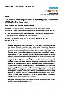
structure was presented by Radenburg, 2013 as shown in Figure 2.2. The micropore size in the final product is a consequence of the primary particle size of the liberated silicic acid, which can be controlled by varying the solution pH, temperature, and silica concentration (Yang, 2003).
5x (5 mm scale bar)
30x (500 micron scale bar)
15kx (100 nm scale bar)
Figure 2.2 SEM images of silica gel used in the ISS CDRA. Note the circle identifying one of the primary particles in the 15kx view (15kx image from http://www.grace.com/EngineeringMaterialScience/SilicaGel/SilicaGelStructure.aspx), other images from Radenburg, 2013).
15
2.1.3.7 Silica Gel Surface Chemistry Hydroxyl (or silanol) groups on the silica gel surface account for an intermediate degree of surface polarity. The surface polarity of silica gel is greater than for activated carbon, but not as high as for zeolites.
As a result, polar molecules are adsorbed
preferentially over nonpolar molecules, yet the bond strength (and thus energy required for desorption) is not as great as for zeolites. Aside from water, silica gels also have good selectivity for alcohols, phenols, and amines. 2.1.3.8 Applications of Silica Gel Two variants of silica gel types are commercially available. The narrow pore (also called high area as well as regular density) silica gel has a greater surface area, 800 square meters per gram vs. 400 square meters per gram for the wide pore type (Grace Davison, 2010). As may be expected from its larger surface area, water capacity is much greater for the narrow pore type. However, as the wide pore type can tolerate liquid water without fracturing, unlike the narrow pore type, and is therefore used as a guard bed in dryers. Silica gel is well suited to molecules that have a high dipole moment and high polarizability, such as water vapor. Silica gel is used to desiccate the air stream prior to CO2 removal in spacecraft life support applications as described later in more detail. The most common commercial uses are shown in Table 1.1. 2.1.3.9 Zeolite History The naturally occurring form of zeolite takes its name from the Greek words meaning “to boil” and “a stone,” based on the observation that steam is produced upon rapid heating of the mineral. It was so named and classified as a new form of mineral in 16
1956 by Axel Fredrik Cronstedt, a Swedish mineralogist (Kuhl and Kresge, 1997). As early as 1840, it was recognized that mineral zeolites could reversibly adsorb water with no change in morphology. F. Grandjean observed gas adsorption in 1909 on chabazite, a natural zeolite. Later observations by McBain on the selectivity of chabazite for gas molecules with sizes below 5 angstroms lead him to call these minerals molecular sieves. However, due to impurity of the mineral zeolites they are less well suited for industrial applications. For example, iron (a common impurity) can strongly affect the catalysis processes (Breck, 1974). A purer form of zeolites became available upon the invention of the synthesis process of zeolites A and X by Milton (1959). 2.1.3.10 Zeolite Synthesis The most common process for zeolite manufacture is the hydrogel process. The primary steps in the hydrogel zeolite synthesis are crystallization, ion exchange, and pelletization. Synthesis of the zeolite crystals starts with a solution of sodium silicate and sodium aluminate in sodium hydroxide. The solution is held in a hydrothermal synthesis autoclave at conditions of pressure, pH, concentration, and temperature specific to the desired zeolite.
Over a period of time, varying from a few hours to a few days,
aluminosilicate gels crystallize out of the solution to form a gel. The zeolite crystals are filtered out of the synthesis liquor prior to undergoing ion exchange in an aqueous solution. Zeolite crystals consist of SiO4 and AlO4 tetrahedrals sharing an oxygen atom to form polyhedral building blocks. These in turn form framework structures such as shown in Figure 2.3a, which repeat to form a crystal lattice resulting in cubic geometries. The
17
primary geometry types are A, X, and Y. Exchanging the cation may be used to change the adsorptive properties of zeolites. For example, the A type with calcium cation, or CaA, adsorbs water and carbon dioxide, while the potassium form, or KA, adsorbs water but not carbon dioxide due to a smaller pore size. Thus the ion exchange step is used to tailor the zeolite crystal for a specific application. The crystals are dried at 150°C prior to the pelletization step. Pelletization of the approximately 2-µm crystals with clay binder is required to reduce flow resistance through a fixed-bed. The most common processes are extrusion to form cylindrical pellets, extrusion followed by rolling to form spherical pellets, and granulation (also to form spherical pellets). The composite nature of the pellets is shown in Figure 2.3b and in the 1kx view in Figure 2.4. However, the open composite structure required for easy gas penetration tends to have a low resistance to attrition and crushing, and weakens due to humidity and/or large temperature excursions (Watson et al., 2015, Knox et al., 2015b). Scanning electron microscope (SEM) images of sorbent pellets used in the ISS CDRA are shown in Figure 2.4. The final steps in the synthesis product are drying at 200°C and calcination at 650°C (Ruthven, 1984).
18
Figure 2.3 (a) Pelletized zeolite pellets, (b) crystals, and (c) framework structure http://www.grace.com/engineeredmaterials/productsandapplications/InsulatingGlass/Siev eBeads/Grades.aspx).
2.1.3.11 Zeolite Surface Chemistry Adsorption in zeolites for non-polar molecules is due in part to van der Waals forces as with silica gels and carbons. However, the forces between zeolites and polar gases (particularly H2O and CO2) are much higher, resulting in superior separation and capacity for polar molecules compared to activated carbon or silica gel. Conversely, high temperatures are also required for desorption. Also, since adsorbed H2O will exclude CO2 adsorption due to the higher polarity of the water molecule, the stream must be desiccated prior to the CO2 adsorption step.
19
Figure 2.4 SEM images of pelletized zeolite 5A used in the ISS CDRA. Individual zeolite crystals are evident in the 1kx views (Radenburg, 2013).
2.1.3.12 Applications of Zeolites Zeolite crystals are unique among sorbents due to their constant pore size. This property allows the zeolite to act as a molecular sieve. The other unique feature of zeolites is their high electric field gradient due to the cations being situated above the negatively charged surface oxides.
This favors a molecule with a high quadrupole
moment, such as water vapor, over carbon dioxide (Yang, 1987). As shown in Table 2.1, there are many commercial separations made possible by both the sieving and polar properties of zeolites. Zeolites are also used in spacecraft life support systems for both the desiccation of air and the subsequent removal of CO2.
20
2.1.4
Equilibrium Capacity Isotherms The most important metric used in evaluation of a sorbent for a gas separation
process is sorbent capacity.
To quantify the capacity of a sorbent for a sorbate,
experimental capacity data are collected on a small amount of sorbent in a closed chamber with sorbate partial pressure and temperature held at constant conditions until equilibrium capacity is attained. In general, a series of these experiments are conducted by varying the sorbate pressure over the desired range while holding temperature constant, resulting in a single equilibrium capacity isotherm. The experiment is then repeated for each temperature of interest. Figure 2.5 shows an example set of isotherms for CO2 on zeolite 5A (Wang and LeVan, 2009).
Figure 2.5 Equilibrium capacity isotherms for CO2 on zeolite 5A, where data points represent test data and the lines represent the Toth fit to the data (Wang and LeVan, 2009).
21
The shapes of isotherms are known to have a dramatic effect on the breakthrough curve shape (Park and Knaebel, 1992). As will be shown in this work, the steepness of an isotherm is a contributing factor in the onset of non-physical behavior in the simulation of breakthrough curves. Isotherms are categorized by their shape into types I through V as shown in Figure 2.6 (Brunauer et al., 1940). The sorbents used in this study concave downward, or type I. This shape is considered favorable, if it leads to a compact wave shape and constant pattern behavior in a breakthrough experiment, whereas the concave downward or type III shape will have a spreading pattern that is undesirable for effective fixed-bed utilization (LeVan and Carta, 2008). Equilibrium capacity isotherms also provide critical input data for a computer simulation. Mathematically, the driving force for adsorption is the difference between the loading of a sorbent particle and the loading that the particle would have if it were in equilibrium with the gas stream. Equilibrium equations are used to fit the equilibrium capacity isotherm data; for example, the Toth equation is shown in Equation (2.3);
n=
ap 1/t
⎡⎣1+ (bp)t ⎤⎦
;
b = b0 exp(E / T );
a = a0 exp(E / T );
t = t0 + c / T ,
(2.3)
where n is the sorbent loading, a is the saturation capacity, p is the partial pressure, b is an equilibrium constant, and t is the heterogeneity parameter. Parameters a, b, and t are temperature dependent as shown, whereas a0, b0, and t0 are system dependent adsorption isotherm parameters. A comparison of the Toth equation and the experimental data are shown in Figure 2.5. The adsorption isotherm parameters are given in Wang and LeVan (2009).
22
Figure 2.6 Isotherm types I through V, where pi is sorbate partial pressure, ni is sorbent loading, and is the sorbate saturated pressure (Brunauer et al., 1940).
2.1.5
Mass Transfer Mechanisms in Fixed-Beds Pelletized sorbents may be used in fixed or fluidized beds. In fluidized beds, the
pellets are transported from an adsorption zone after adsorption is complete to a desorption zone with conditions suitable for removal of the sorbate. In a fixed-bed, as illustrated in Figure 2.7, pellets are retained in a single bed; after adsorption is complete, conditions are altered to encourage desorption to occur. The change in conditions may be a swing in pressure or temperature (termed pressure swing or temperature swing adsorption, respectively), purging in the same direction as adsorption with inert gas (cocurrent inert purge stripping), purging with a reversal of flow direction (counter-current inert purge stripping), or a combination of these such as temperature/vacuum swing
23
adsorption (TVSA) as used for the carbon dioxide sorbent bed in the ISS CDRA. Another method used for example, in the separation of paraffins from gasoline, is displacement purge; in this case, a species that is preferentially adsorbed is used to replace and purge the desired species out of the bed. Distillation is then required to separate the paraffin from the regeneration effluent. This was one of the earliest commercial uses of zeolites (Kuhl and Kresge, 1997).
Figure 2.7 Packed (or fixed) bed of zeolite 13X beads. Photo taken by author.
The physics of the adsorption process in a fixed-bed can be broken down into five general mass transfer modes, described in detail below and illustrated in Figure 2.8. The mass transfer modes are as follows: (1) Convection and dispersion of the sorbate via the carrier gas longitudinally down the packed bed, (2) mass transfer of the sorbate from the 24
free stream through the external fluid film around the zeolite pellet, (3) mass transfer through the pellet macropores, (4) mass transfer into the zeolite micropores through the pore mouth, or barrier resistance, (5) surface migration of molecules from external adsorption sites to sites through the micropores further in the interior of the crystal. Each of the transfer mechanisms is described in greater detail below.
Figure 2.8 Depiction of fixed-bed and zeolite mass transfer mechanisms (Shareeyan et al., 2014).
2.1.5.1 Convection and Dispersion Fixed-beds consist of a non-ordered packing of randomly sized sorbent particles as shown in Figure 2.7. It follows that the resulting flow field is also random with dispersive attributes. Dispersion can include turbulence, flow splitting and rejoining around particles, Taylor dispersion, channeling, and wall effects. For small channels, 25
dispersion can greatly reduce efficiency by broadening the mass transfer zone, yet as discussed later in detail, care must be taken to avoid the non-physical simulation phenomenon resulting from the interaction of a high axial dispersion coefficient and the Danckwerts boundary condition. 2.1.5.2 External Pellet Film Diffusion The diffusion of gas from a free stream into a stagnant film layer, and across a stagnant film layer to the zeolite surface, is based on Fick’s law (see, for example, Bird, Stewart, and Lightfoot, 1960). Although the film resistance is significant for heat transfer from the gas to the pellet, film resistance is insignificant for mass transfer from the gas to the pellet for zeolites due to the dominant resistance in the macropores and micropores (Ruthven, 1984). The film resistance term and those resulting from following mass transfer modes will be lumped together as a single term. Heat diffusion in the film, however, will be determined via correlation and used in the energy balance equations. 2.1.5.3 Mass Transfer Through the Zeolite Macropores The zeolite pellets are composed of the zeolite crystals (the cubic structures in Figure 2.3b and clay binder (the randomly shaped material around the cubes). The spaces between the cubic crystals are the macropores. The macropores are visible as the spaces between crystals in the 1kx images in Figure 2.4. 2.1.5.4 Mass Transfer into the Zeolite Crystal through the Pore Mouth A schematic representation of the framework structure of zeolite A is shown in Figure 2.3c. Sorbate molecules enter into the crystal via the pore mouth, or outermost crystal framework. The effective opening size for zeolite A ranges from approximately 3
26
to 4.5 Angstroms depending on which molecule is acting as the cation in the framework structure. Examples are: potassium for 3A, sodium for 4A, and calcium for 5A (Ruthven, 1984). 2.1.5.5 Mass Transfer into the Zeolite Crystal Interior through the Micropores Full utilization of the zeolite crystal requires movement of the sorbate from the external to interior crystal lattices. However, since the molecules are initially captured by the external adsorption sites, the transfer occurs by a “hopping” or surface diffusion mechanism from one adsorption site to another (Yang, 1987; Ruthven, 1984; Karger and Ruthven, 1992). 2.1.6
Linear Driving Force Model In the LDF model shown in Equation (2.4), the following mass transfer
resistances are lumped into a single mass transfer resistance: external pellet film diffusion, mass transfer through the pellet macropores, mass transfer into the zeolite crystal through the pore mouth, and mass transfer into the zeolite crystal interior. If the mass transfer resistance is assumed to be a single mass transfer mechanism that is dominant and constant throughout the adsorption process, then this approach is valid. Also, it has been established that the LDF model incurs little error for most commercial gas phase cycle adsorption processes when the LDF coefficient is empirically derived (Yang, 1997; Sircar, 2000).
The most commonly used model for adsorption mass
transfer, and the one used in this work, is the LDF model.
∂q = kn (q* q ) ∂t
27
(2.4)
2.2
Emerging Applications of Gas Separations The subject of this work is to refine the methods used to derive mass transfer
coefficients for gas adsorption systems. Although these refinements may be applied to existing gas adsorption systems to increase performance, an even more beneficial application is during the design of new systems, with either newly developed sorbents or where existing sorbents are being newly applied to a separation process. Some emerging applications are described below, both in the commercial and spacecraft life support arenas. 2.2.1
Emerging Applications in the Chemical Processing Industry The separation of air into high purity nitrogen and oxygen is extremely important
in the chemical, processing industry, as these are second and third most produced chemicals respectively. Two innovations have contributed to the significant reduction in cost of oxygen production: (1) the development of the vacuum swing adsorption (VSA) process, and (2) the invention in 1989 of a new zeolite, LiLSX (Yang, 2003; Chao, 1989). The LiLSX zeolite is also under consideration for CO2 removal on spacecraft life support systems due to its high capacity for CO2 at low partial pressures (Knox et al., 2016b). A related sorbent developed for the production of oxygen is AgLiLSX, where a small percentage of silver ions (1%-3%) are exchanged with the lithium ions in the LiLSX zeolite, with a resultant increase in the nitrogen capacity (Chiang, 2002). A combined pressure and vacuum swing adsorption (VPSA) process using 40% Ag-exchanged LiLSX was invented by Whitley (2010). The commercial status of this sorbent and process is unknown.
28
There are a number of other gas separations that may be enabled by emerging sorbents, which will in turn enable future applications, such as purification of hydrogen for fuel cells, and potential enhancements to current applications, such as the use of PSA for recovery of ethylene and propylene from refineries. These are discussed in detail by Yang (2003) and summarized in Table 2.2.
Table 2.2 Gas separation and purification applications enabled by new sorbents (Yang, 2003). Application
Sorbent and Notes
N2/CH4 separation for natural gas upgrading
Clinoptilolite, tinanosilicates by kinetic separation, single-wall carbon nanotubes
CO removal from H2 to < 1 ppm for fuel cell applications
π-complexation sorbents such as CuCl/γAl2O3, CuY, and, AgY
NOx removal
Fe-Mn-Ti oxides, Fe-Mn-Zr oxides, CuMn oxides, multi-wall carbon nanotubes
C3H6/C3H8 (+hydrocarbons) separation
π-complexation sorbents such as CuCl/γAl2O3, AgNO3/SiO2, AgNO3/clays, aluminophosphate
C2H6/C2H6 (+hydrocarbons) separation
π-complexation sorbents such as CuCl/γAl2O3, AgNO3/SiO2, AgNO3/clays
2.2.2
Efforts to Develop Affordable Flue Gas CO2 Capture Systems The separation of CO2 from the flue gas produced by the combustion of coal in
power generating plants is an area of gas separations that has seen an extraordinary amount of research activity recently, and which has a close tie to the sorbents and sorbates studied in work.
In 2009, coal-based power plants provided 45% of the
29
electrical power in the United States. The use of coal is not expected to decrease significantly in the near future; in 2030, coal-based power plants are predicted to provide 44% of the electrical power in the U.S. However, CO2 emissions from coal-based power plants in the U.S. produced 1.7 billion metric tons of CO2 in 2009, constituting 32% of the total U.S. CO2 emissions resulting from human activities (Vora et al., 2013). To reduce CO2 emissions, which is considered responsible for the current global warming trend, the U.S. government began funding the development of technologies for the capture of CO2 from coal-based power plants in 2008. Between 2008 and 2016, the U.S. Congress alone has appropriated more than $7 billion for carbon capture and sequestration (CCS) activities at the Department of Energy (DOE), with CO2 capture activities accounting for approximately one quarter of that budget. For 2017, the DOE carbon capture budget request is the highest yet at $170 million (Folger, 2016). A large portion of this funding has been directed to the development of technologies that would enable cost-effective CO2 removal from coal-based power plant smoke stacks, as currently available commercial CO2 capture technologies are not yet practical for this application. The options under consideration for coal-based power plant smoke stacks (or post-combustion) are shown in Figure 2.9. The current technologies would incur parasitic loads that would reduce power-generating capacity by approximately one-third (Vora et al., 2013). Carbon dioxide capture technologies funded under DOE that could benefit from the methods described in this dissertation are summarized in Table 2.3.
30
Figure 2.9 Key technologies and associated research focus for post-combustion capture (National Energy Technology Laboratory, 2013).
Table 2.3 Carbon dioxide capture technologies funded under DOE (Vora et al., 2013).
Project Name
Project Focus
Sorbent Materials
Process Approach
Technology Maturity
Ref.
Bench-Scale Development & Testing of a Novel Adsorption Process for PostCombustion CO2 Capture
Novel adsorption process
Microporous carbon
TSA, fixed-beds
Bench-Scale, Actual Flue Gas
Jain, 2012
Low-Cost Sorbent for Capturing CO2 Emission Generated by Existing CoalFired Power Plants
Low-cost solid sorbent
Alkalized alumina sorbent
Simulated moving beds
Bench-Scale Elliot, Using Actual 2012 Flue Gas
CO2 Removal from Flue Gas Using Microporous Metal Organic Frameworks
Microporous MOFs
Alumina and Mg/ DOBDC
VPSA
LaboratoryScale, Simulated Flue Gas
Benin, 2012
Recent reviews of carbon capture progress note that further work on sorbents is required in the areas of capacity, kinetics, selectivity, and operational stability. These 31
reviews also include the more recent approach of removal of CO2 from the atmosphere despite the difficulty of doing so at greatly reduced concentrations. In this application, the physisorption candidates are activated carbons, zeolites, and MOFs, or the same candidates as for the post-combustion application (Yuan et al., 2015; Miller et al., 2016). Other recent developments in crystalline molecular sieve development include the silicoaluminophosphates, or SAPO4 sorbents. These molecular sieves have an unusual degree of diversity in the framework structures. SAPO4-34 in particular has shown a high selectivity of for CO2 over other atmospheric gases (Arevalo-Hilalgo et al., 2010). 2.2.3
Spacecraft Life Support Needs for Reduced Mass/Power/Volume Systems The long-term goal for NASA is to enable crewed missions to Mars, first to the
vicinity of Mars, and then to the Mars surface (NASA Headquarters, 2015). These missions present new challenges for all aspects of spacecraft design in comparison with ISS, as resupply is unavailable in the transit phase, and early return is not possible. Additionally, mass, power, and volume must be minimized for all phases to reduce propulsion needs. Mass reduction is particularly crucial for Mars surface landing and liftoff due to the challenges inherent in these operations for even much smaller payloads. In manned space vehicles, CO2 partial pressures have historically been maintained below 7.6 mmHg for short-duration missions (e.g., Apollo or Shuttle flights) and averaging approximately 5 mmHg for long-duration missions (e.g., 30-day Skylab and 180-day ISS missions). However, after 15 years of experience on the ISS, the medical community has gained knowledge on the combined influence of microgravity and CO2 concentrations that are ten times Earth’s normal on human physiology. This greater understanding seems to point towards the need for lower CO2 concentration requirements
32
for future spacecraft, which will drive the CO2 removal system to higher flow rates and greater efficiency (James et al., 2011; James 2013a, 2013b). Recently, it was recognized by the life support community that the current ISS state-of-the-art CO2 removal technology, the Carbon Dioxide Removal Assembly (CDRA), has reliability and capability gaps that must be solved both for ISS and future Exploration missions (Knox et al., 2015a). Technical interchanges with the adsorption industry and academia were conducted to determine the appropriate development path to achieve the system reliability and capability needed for a crewed mission to Mars. The following goals were established: 1. Select superior desiccants and CO2 sorbents for ISS CDRA. Criteria for selection include performance, structural stability, and sensitivity to contamination.
Only
sorbents compatible with the current ISS CDRA hardware are under consideration. 2. Using the ISS CDRA design as a basis, complete design of a next-generation CO2 removal system with appropriate attributes for a 2-year mission with no resupply. Implement this design in the fabrication of a technology demonstration to fly on ISS by 2019. 3. Down-select between promising alternate technologies after further development as required to bring the candidates to similar technology levels. Complete design of a next-generation CO2 removal system based on the selected technology with appropriate attributes for a 2-year mission with no resupply. Implement this design in the fabrication of a technology demonstration to fly on ISS by 2019. All three goals require accurate selection of the superior sorbent (zeolite, silica gel, alumina, solid amine, etc.). However, goals 2 and 3 also require selection of the
33
superior process (four-bed molecular sieve, pressure swing adsorption, temperature swing adsorption, etc.) coupled with the superior sorbent format (clay-bound pellets, polymerbound monolith, honeycomb monolith, sorbent coated metal, etc.). 2.3
Virtual Design of Gas Separation Systems The fundamental performance aspects of many sorbents (such as surface area,
equilibrium working capacity, and selectivity) have been used as metrics to rank their potential superiority in a particular application. However, these metrics can provide conflicting data regarding which sorbent is superior, and have been shown to be unreliable in predicting superiority in process performance for post-combustion CO2 capture (Haghpanah et al., 2014). For spacecraft CO2 removal, an equally complex application, standard figures of merit alone will not be used to optimize the processes involved. Rather, computer simulations that capture the key physics of the process, including coupled heat and mass transfer in porous media, must be applied. A large number of parametric simulations (also referred to as virtual tests) are required to converge on the optimal solution. Parametric hardware testing could also be employed, of course, but would be prohibitively expensive and time-consuming, severely limiting the number of options that can be explored. In Figure 2.10, the integrated optimization approach is shown. Essentially, there are three steps in performance optimization: the first to screen out the worst performing sorbents, the second to obtain the “Startup Performance Optimization,” and the third to obtain the final “Ranking of Sorbent/Process Systems.”
34
Figure 2.10 Integrated optimization approach flowchart (Knox et al., 2015a).
35
In the second step, sorbent and process characteristics are determined and simulated. Process parameters such as bed sizes, flow rates, cycle times, etc. are varied in a series of virtual tests in order to optimize the performance of each candidate process and sorbent combination. The top performing combinations are subjected to hardware testing to confirm results and validate the simulation. If required, simulation refinement and hardware tests are repeated until validation is successful. Upon completion of this step, the optimal process, sorbents, and process parameters are determined based on the characteristics of unused sorbents.
This is the “Startup Performance Definition” in
Figure 2.10. The number of sorbent/process systems carried forward to step 3 will depend on their relative ranking at this point. As the ISS CDRA and commercial experience have revealed, long-term operation can lead to sorbent degradation, including capacity losses and attrition. These factors will be accounted for in the third step, where a second round of parametric virtual testing is conducted. As different sorbents have varying sensitivities to contamination and varying long-term stability, the initial ranking may change when end-of-life performance, flow losses, and maintenance requirements are factored in. Development of an accurate mathematical model of these candidate systems is required in order to optimize design parameters such as bed size, cycle time, heater power and temperature set point, and vacuum pump parameters for the particular mission scenario without resorting to exhaustive (and expensive) hardware testing. The results from these studies will form the basis for the down-selection process shown in Figure 2.10. However, schedule constraints dictate that the computational time requirements are minimized, both due to the large number of system optimizations required for down-
36
selection. Moreover, since for these cycle systems, a periodic state must be achieved for any one test case to be completed, which can require running a simulation for many cycles. 2.4
Literature Review of Adsorption Models Appendix A provides the results of a literature survey of recent fixed-bed gas
adsorption models. Those selected for inclusion in Appendix A were published in the year 2000 or later, are generally based on either the 1-D axially dispersed plug flow equation or the 1-D plug flow equation, and include a description of the experimental data used to validate the model. The subset of models meeting these criteria represents about half of the original set, but provide a representative cross-section of all those published. The data provided in Appendix A is summarized below. 2.4.1
Applications The model applications range from post-combustion carbon capture (models 1, 3,
10, 13, 15, and 16) to industrial purity (2, 9, 11, 12) and dehumidification applications (4, 5, 7, 8, 18, and 19) to spacecraft CO2 control (3, 6) to thermochemical energy storage (17). Thus, it is evident that the 1-D modeling approach is used across many disciplines. 2.4.2
Experimental System The experimental system in this context refers to the sorbate/sorbent system. The
use of standard zeolite types (3A, 4A, 5A, 13X, ZSM-5, and silicalite) predominates, representing one or more of the sorbents in 15 of the 19 publications. Carbons (including carbon molecular sieve) show up in six publications, silica gel in three, and hydrotalsite in one publication. It is clear that, although interest does exist in emerging sorbents, the
37
standard zeolites, silica gels, and carbons capture the greatest interest in the model-based design of new and enhanced processes. 2.4.3
Spatial Dimensions 1-D models are used in 16 of the 19 publications represented. As stated earlier,
although the 2-D models reviewed (models 4, 6, and 17) provided important information about the actual 2-D flow in small columns, none were actually applied to a model-based process design. The design and optimization of a cyclic process often requires simulating many repeated cycles (in order to attain a cyclic steady state response) such that the shorter simulation execution times required for a 1-D model are needed. 2.4.4
Tube Inner Diameter/Particle Diameter The tube inside diameter (ID) to particle diameter ratio provides an indication of
the impact of the tube wall on the overall flow through the tube. Since the particles, regardless of geometry (beads, pellets, or granular), cannot nestle at the flat wall surface, the packing density is lower near the wall. The void fraction approaches unity at the wall, and decreases until it approaches the core void faction at about five particle diameters from the wall (Nield and Bejan, 1992). Due to the higher void fraction at the wall, wall channeling (or higher flows) occurs in that location. For fixed-bed adsorption, the combination of lower sorbent density and higher flow result in earlier breakthrough at the walls. The effect of wall channeling is generally considered negligible at a tube to particle diameter ratio of 20 (Richardson et al., 2002). However, it will be shown in this work that, even for a ratio of 20, wall channeling is observed. Nearly all the testing reported on in the publications in Appendix A was performed with test apparatus at or below a value of 20 for the tube to particle diameter 38
ratio, with only publications 3, 14, and 17 being significantly higher. Most publications have a much lower ratio. It is evident that subscale testing such as breakthrough analysis is generally performed in small columns, which reduces both the sorbent required and experiment time. As a result, appropriately accounting for the wall channeling via an approach such as that shown in this work is required for accurate empirical derivation of the mass transfer coefficients discussed next. 2.4.5
Gas to Particle Rate Expression The modes of mass transfer from the gas to the adsorbed state were discussed in
section 2.1.5. As discussed, the LDF model shown in Equation (2.1) may be used to lump the four mass transfer mechanisms from the free stream to the interior of the zeolite crystal into one or two linear expressions. Most (12 of 19) of the models studied employed the LDF approach. Another approach used in publications 1, 7, and 9 is to condition the LDF term based on local concentration, temperature, or loading. The models in publications 4, 11, and 15 use variations of the bi-disperse approach for composite zeolite particles, which conceptually models both the diffusion in the macropores between the zeolite crystals and the diffusion within the zeolite crystal. Finally, the model described by publication 13 uses a variant of the LDF equation, the quadratic driving force (QDF) equation.
Here, the terms inside Equation (2.4) are
squared as shown in Equation (2.5):
∂q = kn (q*2 − q 2 ) . ∂t
39
(2.5)
It should be noted that the approach presented in this work to obtain an empirical fit of the gas to particle rate coefficient is independent of the gas to particle rate model used. 2.4.6
Method to Determine Gas to Particle Rate In the publications examined, 11 of 19 used breakthrough analysis to determine
the gas to particle mass transfer rate. Breakthrough analysis consists of comparing the results of an adsorption breakthrough test with the model results and fitting the mass transfer coefficient to best match the test data.
Publication 1 also examined the
desorption profile, and found that modifications to the simple LDF approach was required.
Various approaches were used to estimate the LDF value in five of the
publications.
These estimates are based on equations that sum the film resistance,
micropore diffusion, and micropore diffusion or a subset thereof. However, each of these terms includes a diffusion term that must be empirically obtained, either through breakthrough analysis or other testing. For the publications reviewed, it was evident that a breakthrough analysis tended to provide a better match between model results and test data than the estimation approach, perhaps because the breakthrough analysis accounts for the all of fixed-bed physics. 2.4.7
Axial Dispersion Axial dispersion was included in 14 of the 19 publications reviewed. The most
common correlations used to estimate axial dispersion were that of Edwards and Richardson 1998 and Wakao and Funazkri 1978. These two correlations are also used in this work to bound the full range of values calculated by the five correlations considered in Chapter 4. Note that the value obtained from the Wakao and Funazkri correlation is 2 40
to 3 times greater than that obtained from the Edwards and Richardson correlation, thus the choice of an axial dispersion correlation provides a limited capability to fit the dispersion value. 2.4.8
Internal Profile Shown? In Chapter 5, this work will show that for a specific sorbate/sorbent system
(H2O/5A) and by extension, other systems with a high distribution factor (which indicates the steepness or curvature of the equilibrium adsorption isotherm), non-physical simulation behavior, i.e., sharpening of the concentration front just prior to breakthrough, can occur even using commonly used correlations for the axial dispersion coefficient. This non-physical behavior is only evident upon inspection of the internal concentration history, but only the breakthrough curve is generally examined for the fitting process. For the publications reviewed, 13 provided only the breakthrough curve, and thus provided no evidence that the internal profile showed a physical behavior. Of these 13, 7 simulated H2O/zeolite systems, which have a high distribution factor and thus a high potential for non-physical behavior.
41
CHAPTER III
3. EXPERIMENTAL
The development of computer simulations of adsorption processes requires two key experimental inputs. The first is capacity of the sorbent under consideration for the sorbate of interest when at equilibrium with a gas held at constant temperature and sorbate partial pressure.
A series of these capacity measurements, or equilibrium
adsorption capacity isotherms, may be fit to a standard correlation as described later. In the computer simulation, the driving force for adsorption is the difference between the current sorbent loading and the loading that would be attained if the sorbent were equilibrium with sorbate in the surrounding gas stream. However, the sorbent does not come to equilibrium with the surrounding gas stream immediately.
The second experimental input provides a limiting rate of
adsorption, or mass transfer coefficient. A standard method for derivation of this mass transfer coefficient is via breakthrough testing and comparison of the test results with the computer simulation. In order to support the development of computer models and simulations of the ISS CDRA, a breakthrough test stand, the Molecular Sieve Material Bench Test (MSMBT), was fabricated at NASA’s MSFC in the early 1990’s (Knox, 1992a; Knox, 1992b; Mohamadinejad, 1999; Mohamadinejad et al., 2000).
42
3.1
Objective The MSMBT test objectives are to characterize the adsorption material by
mapping the dynamic adsorption and desorption characteristics for a range of flow rates and adsorbent concentrations. Characterization of both single-gas adsorption (CO2, O2, N2, and H2O with He carrier gas) and multi-gas adsorption (combinations of CO2, H2O, N2, and O2) was required. Results from single gas adsorption of CO2 and H2O on zeolite 5A, is reported on in this document.
Inlet gas concentrations (held constant for a
particular test) were varied in the range expected in manned spacecraft (0.7% to 1.5% by volume). Helium was chosen as the carrier gas since is not appreciably adsorbed by molecular sieves. 3.2
Test Apparatus
3.2.1
Packed Column
A small packed column with approximate dimensions of 2 inches in diameter and 20 inches long (Figures 3.1 and 3.2) was used during adsorption testing. Actual ISS CDRA CO2 removal system beds have cross-sectional areas of about 80 square inches; this size would have required a prohibitive quantity of the helium carrier gas. The test flow rate was scaled to give gas velocities similar to that in the flight-like beds. Instrumentation of the packed column includes temperature probes and sampling tubes for measurements at sorbent material endpoints and one intermediate point. Two duplicate columns were fabricated of two-inch OD, 1/16-inch thick stainless steel 24 inches in length. Compression fittings (reducing unions with copper crush washers) provided a gas-tight enclosure. A spring seated on the union at one end maintained compaction of the bed material. The columns were packed using stainless steel, 40 mesh screens for containment of sorbent material and separation from the glass beads. Following placement of 43
the glass beds to the proper level, filling of the test columns with adsorbent proceeded by securing the columns to a shaker table, pouring the sorbent material into the column in 200 ml batches, and vibrating for 10 seconds. Thermocouple probes and sampling tubes were inserted as required and aligned visibly during the filling process. When the filling process was complete, the second union nut was tightened until the seal quality was confirmed with a helium leak-check apparatus.
Figure 3.1 (a) Breakthrough test apparatus of Knox (1992) and (b) cross-sectional view of typical sampling location.
44
Figure 3.2 Fixed adsorbent bed cutaway (Knox, 1992b).
The adsorbent was a commercial zeolite 5A, Grace Davison Grade 522, in bead form. The adsorbent (Finn and Ho, 1995; Radenburg, 2013) and experimental apparatus properties are listed in Table 3.1.
Table 3.1 Properties of the adsorbent and fixed-bed.
Adsorbent
Fixed-bed
Pellet radius (spherical)
Rp = 1.16 mm
Particle density
ρs = 1180 kg m-3 -3
Bed height
L = 0.254 m
Bed internal diameter
Ri = 47.6 mm
Column wall thickness
l = 1.59 mm
Skeletal density
ρsk = 2040 kg m
Heat capacity
cps = 920 J kg-1 K-1
Wall heat capacity
cpw = 475 J kg-1 K-1
Langmuir surface area
AL = 463 m2 g-1
Wall density
ρw = 7833 kg m-3
45
Brisk-Heat heat traces (12-foot length with 8.6-watt density per inch) were wrapped around the stainless steel tubing for the thermal desorption procedure. Adiabatic bed conditions were desired for the initial phase of testing, and to aid in the thermal desorption process. The column was first covered with Mansfield Q-fiber felt insulation, and then wrapped with a thermal blanket of Mansfield Min-K material. The insulation, approximately 1 inch thick in all, was used with satisfactory results. 3.2.2
Sensors Instrumentation provided for continuous measurement of packed column inlet and
outlet CO2 concentration via Horiba model APBA-250E infrared CO2 sensors. Flow rate was measured at various points with Porter and Edwards brand thermal mass flow meters, dew points via General Eastern optical dew point monitors (model Hygro-M1, with sensor 0111D), and pressure via a Heise digital pressure indicator and Viatran pressure transducers.
Manufacturer-provided data for sensor accuracy and repeatability is
provided in Table 3.2. The location of sensors and other equipment comprising the adsorbing apparatus are shown in Figure 3.3.
Table 3.2 Instrumentation with manufacturer-provided accuracy and repeatability.
Sensor Type
Sensor
Accuracy ± 1.0% full scale
Repeatability
Flow meter
Porter 250
Dew point sensor
General Eastern 1111H ± 0.2C of reading
± 0.05C of reading
Pressure sensor
Viatran
± 0.25 full scale
± 0.1 full scale
Thermocouple
Omega T-type
± 1.0C of reading
Gas standard
N/A
± 1.0% of concentration
46
± 0.2% full scale
Figure 3.3 MSMBT adsorption schematic (Knox, 1992b).
The gas chromatograph (GC), a Shimadzu GC-14A with CR601 integrator, was used to sample at five sample port locations to determine gas constituent volumetric fractions during the adsorption runs. Figure 3.2 showed the location of sample probes 2, 3, and 4. Sample probes 1 and 5 are at the inlet and outlet of the column, respectively, as shown in Figure 3.3. To enable automated sampling at the five sampling locations, a Valco multi-position electric actuator (model E6) and six-port gas sampling valve were installed. The sixth port was used for the desorption apparatus. In addition, a Valco 2position electric actuator (model E60) and sampling valve automatically controlled the sequence of purging of sampling lines and introduction of the gas sample from the constant volume loop to the GC column. To maintain constant pressure at the GC constant volume loop, a vacuum pump pulled the gases through the sample lines. 47
Different pressures at the sample port and different pressure drops in the sample lines were accommodated by adjusting a metering valve for consistent flow rate. A CR601 BASIC program was written for automated control of the GC and sample port selection. The GC proved essential during the testing. The GC could receive gas from five sample port locations and determined gas constituent volumetric fractions during the adsorption runs. The infrared CO2 sensors, intended to provide a continuous measurement at the outlet of the column, did not provide reliable data during the early portions of a test run due to the very low partial pressures at the outlet. The infrared sensor was difficult to calibrate for the He carrier gas due to this low partial pressure inconsistency. Therefore, the GC was used as the primary instrument for measurement of gas constituent volumetric fractions. The dew point sensors were limited by a minimum frost point of approximately -10°C (14°F). Measurements on the GC were found to be consistent down to the tens of parts per million range. 3.2.3
Data Acquisition Data from the continuously measuring sensors were acquired with a
Macintosh IIx computer running the LabVIEW II data acquisition and control software. The flow controller flow rates were also set through LabVIEW. Strip charts allowed monitoring of flow rates, inlet and outlet CO2 partial pressures, and dew point conditions during the test. All data were continuously logged to an ASCII data file and could be accessed real time through a separate plotting package. 3.2.4
Support Equipment Supporting equipment for the test included Porter models 250 and 201 thermal
mass flow controllers (PID controlled solenoid valves with thermal mass flow meter 48
input signal) to obtain the proper inlet constituent volumetric fractions. Pressurized “K” bottles supplied all gases. Ultra-high purity He (99.9999% pure) and high purity CO2 (99.8% pure in the liquid state) was used for the first phase of testing. Helium is preferred since it does not appreciably adsorb onto the zeolite sorbents tested. To control temperatures and dew points at the inlet, a saturation column was used for introduction of water vapor into the gas inlet stream. This column was, like the packed columns, 2 inches in diameter by 24 inches long, but customized with the required fittings and filled with beryl saddles to increase gas retention lime. A gas/liquid heat exchanger reduced the dew point to a specified level and provided control of inlet temperature.
A NESLAB Instruments Coolflow refrigerated recirculator supplied
cooling water to the heat exchanger. 3.3
Procedures
3.3.1
Adsorption Procedure Preparation for adsorption test runs included placement of the test column into the
adsorption apparatus and connection of the quick-disconnect fittings. Flow rates were set and allowed to stabilize with flow bypassing the column. With all conditions stable, the bypass valve was turned to initiate flow through the bed coincident with setting the data acquisition clock to zero. Gas chromatograph sampling, with the integrator clock reset to reflect test elapsed time, was then initiated using the CR601 BASIC routine. Quickdisconnects on the sample ports 1 through 4 were connected only as required to prevent excessive gas loss from the remainder of the column. Sample port 5 was left attached throughout the test. Testing continued until the outlet CO2 or H2O concentration closely approached the inlet concentration. 49
3.3.2
Desorption Procedure Following bed packing, and before each adsorption test run, the packed columns
were subjected to a desorption process. Shown schematically in Figure 3.4, the primary desorption method was heating while purging with nitrogen or helium gas. Heat was applied to the column with Brisk-Heat heat traces wrapped around and in contact with the stainless steel tubing. Due to the large unions and end effects, the ends of the column were observed to be cooler than the center. The heat trace was wrapped more at the ends to help counter this effect. Mansfield Q-Fiber felt and Min-K insulation wrapped around the column insured that most of the heat from the trace heated the bed pellets.
Figure 3.4 MSMBT desorption test apparatus (Knox, 1992b).
50
Due to thermal end effects of the columns, it was not possible to maintain the desired minimum desorption temperature (316°C) throughout the bed. A Eurotherm 808 temperature controller controlled the center point of the column at the set point temperature. The cooler inlet gas also reduced temperatures at the inlet end even at low (5 standard liters per minute or less) flow rates. Gas pre-heaters were used, though with little effect since the inlet gas could not be heated above 204°C due to the temperature limitation of the Swagelok Quick-Connect couplings. The problem was resolved by configuring the bed for two-way flow during desorption. Temperatures in the downstream half of the bed exceeded 316°C (temperatures up to 400°C were observed) due to the heat convection of the flow. Flow in one direction was continued until GC sampling confirmed bed desorption (concentrations of less than 20 ppm CO2 and N2 were noted). Flow in the alternate direction then continued until temperatures in the new downstream half exceeded 316°C and the GC samples again confirmed desorption. Nitrogen gas was used for economy in the initial stages of desorption, followed by ultra-high purity helium gas to remove the nitrogen and allow complete bed desorption. Vacuum and thermal conditioning was an alternate technique examined for bed desorption. A KNF model N035.3 SVP diaphragm pump reduced pressures in the bed to 2.2 kPa with accompanying heating via the heat trace. Although somewhat successful for rough desorption, the relatively high vacuum pressure was not sufficient to complete the process alone, and subsequently desorption was performed with the thermal/purge method described above.
51
3.4
Analysis to Determine Experimental Uncertainty To appropriately apply the test data generated by the apparatus described above,
whether for the interpretation of observed physical phenomenon or for computer simulation verification, the degree of uncertainty in the test results must be estimated. In this section, the data collection techniques are discussed in greater detail as required to describe the propagation of sensor errors via the data reduction equations.
This is
followed by the analysis used to estimate the uncertainty of the reported values of concentration and temperature. The complete uncertainty analysis performed in Mathcad 3.1 is provided in Appendix B. 3.4.1
Carbon Dioxide Breakthrough Data Reduction Procedure Concentration data were obtained for the CO2 breakthrough tests using a GC with
a temperature conductivity detector (TCD). The GC was calibrated for CO2 using a gas standard with 0.39994% CO2 in nitrogen. During the CO2 breakthrough tests, it was observed that there was a variation in the inlet concentration as measured by the GC and that this variation could be correlated with changes in inlet pressure.
Pressure variations at different ports is due to the
differences in the differential pressure, since the downstream bed length is different at each sample port. To correct for the variation in GC concentrations, pressure at each port was recorded prior to each test with nitrogen flowing at the same flow rate as during the test. Gas chromatograph measurements were then taken using a certified CO2 standard of 0.39994% in nitrogen. While performing the GC analyses, the calibration gas pressure was varied with the K-bottle regulator. Based on these data, a relationship between total
52
pressure and GC area was obtained. This relationship was used to determine a unique calibration value for each sample port. Generally, a one- or two-point calibration of the GC is performed, where a gas standard with a known percentage of the gas of interest is injected into the GC and the resultant area measured. Since the area corresponding to a gas with zero concentration will be zero, the appropriate calibration curve is a line through the origin with the slope defined by the ratio of the calibration gas percentage to GC area. The GC area obtained during breakthrough testing is then multiplied by the slope or ratio to obtain the gas percentage. As mentioned previously, variations in the GC area with total pressure were observed for the same calibration gas.
To adjust the GC results, a correlation is
developed to correct for total gas pressure at the port location of interest. As a result, the conversion from the GC measurement (area) to partial pressure of CO2 requires the following steps: 1. For each port pressure, find the value of GC area that corresponds to the calibration gas percent CO2. 2. Convert GC area for each test point to CO2 percentage. 3. Convert from CO2 percentage to CO2 concentration for each test point. For step 1, a linear correlation was developed based on GC area and pressure measurements based on the data shown in Table 3.3.
Step 2 uses a single point
calibration based on step 1 and the local port pressure. The data reduction equation for step 3 requires the total pressure and temperature.
53
Table 3.3 Test data taken to determine calibration constants for differing pressures.
Gas Bottle Pressure, psia
Gas Chromatograph Area
14.9
12036 12048
15.3
12309 12335
To calculate the slope, equation (3.1) is used:
m=
GC2 − GC1 P2 −Y1
(3.1)
where m is the slope, P1 and P2 are the low and high pressure settings at the calibration gas bottle regulator, and GC1 and GC2 are the gas chromatograph areas measured at the low and high pressure, respectively. To determine the GC area that corresponds to each sample port pressure, equation (3.2) is used: GCcal = m ( Pcal − P1 ) + GC1 ,
(3.2)
where GCcal is the area corresponding to sample port pressure Pcal. To convert from GC area to CO2 partial pressure, equation (3.3) is used:
fcal =
GS Pcal , GCcal
(3.3)
where fcal is the conversion factor from GC area to CO2 partial pressure and GS is the volume fraction of CO2 in the gas standard (calibration gas). The final equation used to 54
convert from GC area to CO2 concentration is a form of the ideal gas law as shown in equation (3.4):
c=
f cal GC , RT
(3.4)
where c is the CO2 concentration, R is the ideal gas constant, and T is the local gas temperature. 3.4.2
Carbon Dioxide Breakthrough Test Uncertainty Analysis The objective of this analysis is to determine the uncertainty in the reported
results of CO2 concentration.
The uncertainty analysis must take into account the
propagation of errors due to all equations used to convert the GC results, expressed as the area under the curve of the chromatogram for the gas of interest, to CO2 concentration. This analysis must also account for errors in the temperature and pressure measurements as well as the error in the gas standard reported percentage. For this analysis, the relative standard uncertainty of the ideal gas constant (5.7 x 10⁻⁷) may be neglected as it is orders of magnitude below the next smallest uncertainty (Mohr, 2015). The uncertainty of each of the remaining variables is discussed below. In all cases, manufacturer’s data on the appropriate sensor model is used in the analysis, as the test stand is not available, thus eliminating the option of performing direct calibration checks on the actual sensors. An uncertainty value for the CG area is not provided by the manufacturer. An estimate may be made by calculating the standard deviation of the sample population (Coleman, 2009) based on the data from Table 3.3 via Equation (3.5):
55
1
⎡ 1 N ⎤2 SX = ⎢ Xi − X )⎥ = 18.38 , ( ∑ ⎣ N −1 i=1 ⎦
(3.5)
where SX is the standard deviation, N is the number of individual readings of Xi and
is
the sample mean. Since this is a (very) small population of two samples, the value of t corresponding to one degree of freedom is large, and results in a large value for the 95% confidence limit for the high pressure GC area and for the relative uncertainty:
;
.
(3.6)
To consider whether this magnitude of random uncertainty is appropriate or inflated due to the inherent uncertainty in a small sample, a literature search on the uncertainty of other GCs using TCD was conducted. In the natural gas industry, CO2 in the raw gas must be removed. Zuas (2015) reported that the percent relative standard deviation for CO2 as detected by a GC with TCD over a wide range of GC flow rates varied from 0.10% to 0.40%. Sutan (2013) found that combined relative uncertainty for CO2 analyzed with a GC and TCD to be 0.3594%. Based on these references, a relative precision uncertainty of 0.4% is applied in this analysis. Pressure transducer uncertainty is provided as a percent of full scale (Viatran 2010), which is taken to be 30 psia. Based on an email exchange with the manufacturer (Jerry Webb, e-mail communication, November 23, 2015) the specifications provided in Table 3.2 provide a pass/fail criterion as opposed to a statistical confidence interval. Thus, the manufacturer specifications are considered to be maximum values (3 standard deviations) following the approach of Nakos (2004). Errors are normalized to 2 standard deviations as per Lipak (1995). 56
The uncertainty associated with calibration gas, or gas standard, is considered next. For the bias error associated with Matheson standards, a 95% confidence interval is specified by Geib (2005). The gas standard typically used for testing of this type is a high grade standard.
The higher grades for Matheson and Airgas have an overall
uncertainty of 1% in this CO2 partial pressure range. (Matheson, 2007; Airgas 2015). For the uncertainty associated with the measured temperature values, the Omega value of ±1°C could be used (OMEGA, 2010). However, experience in other testing indicates that higher accuracy is generally achieved for standard T-type thermocouples. Testing was recently conducted on 5 T-type thermocouples using a drywell calibrator and a thermistor probe (Croan, 2015).
The thermocouples were calibrated at five
temperatures, from 25°C to 100°C. The uncalibrated thermocouple readings from the data acquisition system were compared with the thermistor probe. The thermistor probe uncertainty is negligible; it is shown by the manufacturer as ±0.01°C calibration uncertainty with ±0.01°C drift and ±0.005 repeatability per year (Fluke, 2015). Based on the thermocouple error analysis shown in Appendix B for the temperature range of the CO2 breakthrough test, reasonable uncertainties are
and
. To
account for installation errors, the values shown are twice the calculated 95% confidence interval for both bias and precision uncertainty. The Monte Carlo Method, or MCM, was used for the uncertainty analysis of the CO2 concentration test results following the approach of Coleman (2009). Convergence of the method was reasonably assured by using 10,000 iterations. Error evaluation for each of the 41 data points must be performed individually due to individual variations in GC area and temperature. All error distributions are assumed to come from Gaussian
57
distributions, and are created via the Mathcad “rnorm” function, which returns a vector of m random numbers having the normal distribution.
Variables GC1 and P1 have a
common correlated systematic error, and thus the systematic uncertainty distribution is calculated prior to the assembly of the uncertainty distribution for these variables as required. Data reduction equations (3.1), (3.2), and (3.3) were used to establish the uncertainty in fcal for each of the four port locations at each iteration. Data reduction equation (3.4) was then applied for each of the 41 GC area data points along with the current temperature at that port to determine the 95% confidence interval uncertainty for each CO2 concentration data point. The relative uncertainty for the concentration measurement was calculated in Appendix B to be approximately 1.2% of the concentration. A typical distribution is shown in Figure 3.5; here the blue line shows a normal distribution based on the mean and standard deviation. It is noted that the concentration uncertainty, shown by the red bars, follows a normal distribution. The callouts show the values for one standard deviation about the mean (0.331 mol per cubic meter).
Figure 3.5 Typical uncertainty distribution for a CO2 concentration measurement. 58
The uncertainty of the flow controller used to regulate the nitrogen gas flow was examined next (Porter Instrument Division, 2012). Based on phone conversation with the manufacturer (Patrick Flaherty, phone conversation, December 11, 2015), the specifications provided in Table 3.2 provide a pass/fail criteria as opposed to a statistical confidence interval.
Thus, the manufacturer specifications are considered to be
maximum values (3 standard deviations) following the approach of Nakos (2004). Errors are normalized to 2 standard deviations as per Lipak (1995). The resulting uncertainties liter/minute and
for a 95% confidence interval are The overall uncertainty is then
liter/minute.
liter/minute. The relative uncertainty is
1.2%. Experimental uncertainty in the temporal dimension for the breakthrough concentration and temperature data can be attributed primarily to uncertainty in the flow controllers. Due to the complexity of the adsorption process, the effect of flow rate changes on the timing of the experimental results may be most accurately estimated by using a computer simulation of the breakthrough test. The simulated inlet flow rate was varied two sigma above and below the flow meter set point for this analysis. Simulation results with flow rates varied for CO2 breakthrough test are shown in Figure 3.6. Each of the figures has three concentration or temperature curves. The center curve in each figure is the result with the set point flow rate. The curve that is earlier in time is the result from setting the flow rate lower by 2 sigma. The curve that is later in time is the result from setting the flow rate higher by 2 sigma. The average relative uncertainty in time resulting from the flow meter with a relative uncertainty of 1.2% is
59
1.30%.
Each of the uncertainties associated with the CO2 breakthrough test is
0.1692
Gas Temperature (K)
Gas Concentration (mol/m3)
summarized in Table 3.4.
0.169 0.1688 0.1686 0.1684 0.1682
304.08 304.06 304.04 304.02 304 303.98 0.375
0.171
Gas Temperature (K)
Gas Concentration (mol/m3)
0.3420.3440.3460.348 0.35 0.352
0.1705 0.17 0.1695
0.38
0.385
305.05 305 304.95 304.9
0.169 0.7
304.85
0.705 0.71 0.715 0.72
0.74
Time (hours)
0.75
0.76
Time (hours)
Figure 3.6 Temporal variation in CO2 breakthrough test due to uncertainty in flow meter: Variation in concentration (left) and temperature (right) at midpoint (top) and exit (bottom). Table 3.4 Estimated uncertainty for CO2 breakthrough test data based on a 95% confidence interval.
Data Element
Uncertainty
Temporal Uncertainty
±1.3%
Concentration Uncertainty
± 1.2%
Temperature Uncertainty (K)
± 0.42 K
60
3.4.3
Humidity Breakthrough Test Uncertainty Analysis The objective of this analysis is to determine the uncertainty in the reported
results of water vapor concentration. The uncertainty analysis must take into account the propagation of errors due to all equations used to convert the GC results, expressed as the area under the curve of the chromatogram for the gas of interest, to water vapor concentration. This analysis must also account for errors in the temperature and pressure measurements as well as the error in the chilled mirror due point sensors used for GC calibration. For this analysis, as for the CO2 breakthrough uncertainty analysis, the relative standard uncertainty of the ideal gas constant (5.7 x 10⁻⁷) may be neglected as it is orders of magnitude below the next smallest uncertainty (Mohr, 2015). uncertainty of each of the remaining variables is discussed below.
The
Once again
manufacturers’ data on the appropriate sensor model are used in the analysis, as the test stand is not available, thus eliminating the option of performing direct calibration checks on the actual sensors. Concentration data for the humidity tests were also obtained with the GC. The GC was calibrated for humidity using a General Eastern 1111H chilled mirror dew point sensor with Hygro-M1 electronics. Helium flowed through a temperature-controlled gas sparger to provide a gas stream at constant humidity. Sparger outlet humidity was measured with the dew point sensor. The GC sampled this gas stream to obtain an area measurement. This process was repeated twice at each of the three humidity settings to obtain a total of six area measurements as shown in Table 3.5.
61
Table 3.5 Gas chromatograph calibration data for water vapor.
Water Vapor per Dew Point Sensor (Pa) 530.9
Gas Chromatograph Area 9654 9667 22579 12335 36444 36343
1278.4 2090.8
The conversion from the GC measurement (area) to vapor pressure of H2O requires the following steps: 1. Convert dew point calibration measurements (as measured by the hygrometer) to vapor pressure. 2. Determine the conversion factor from GC area to H2O vapor pressure. 3. Convert from H2O vapor pressure to H2O concentration. For step 1, the Hardy formulation (Hardy, 1998) is used. Step 2 uses a three-point calibration to find a conversion factor. The data reduction equation for step 3 requires the vapor pressure and temperature. The Monte Carlo simulation approach is used to determine the uncertainty for each step of this analysis. Conversion to vapor pressure is via the Hardy (1998) formulation.
This
conversion incurs less than 0.02% error in the worst incident compared to Table 3 in section 6.5 of the ASHRAE Handbook Fundamentals (Parsons, 1997). Based on the 1/4 rule of thumb, where 1/4 is the ratio of the uncertainty that may be neglected to the largest uncertainty (Coleman, 2009), this error is considered negligible.
62
The dew point sensor uncertainty (Optica, 2008) is provided without specification of the associated confidence interval. The manufacturer specifications are considered to be maximum values (3 standard deviations) per Nakos (2004). Errors are normalized to 2 standard deviations based on the approach suggested by Lipak (1995). The bias errors used for the three calibration measurements will be correlated. For the Monte Carlo analysis, this means a common distribution for the error should be used in the calculation of the measurement distribution, so it is determined prior to the measurement distributions. The random (precision) errors will not be correlated and so are calculated individually for each measurement. Gas chromatograph area data for each of the dew point calibration points are provided in the test data sheet (Mohamadinejad, 1995). As this is a calibration, the bias error is accounted for in the dew point sensor error. However, the GC repeatability should be considered. For this limited set of data, repeatability is calculated using the t value for N = 2 (Coleman, 2009). Once again equations (3.5) and (3.6) are used to calculate relative uncertainties of 1.2%, 0.67%, and 2.5% for the three vapor pressure readings given Table 3.5. However just as in the CO2 calibration case, these values will be biased high due to the large value of t. As described earlier, a relative uncertainty of 0.4% is more typical for CO2; however, no similar literature was found providing typical values for H2O analyses. Another approach is the commonly used single point calibration. Here, we use only the middle point, the first calibration point above the magnitude of the GC area (about 14,000) in the actual test, to allow use of interpolation rather than extrapolation. The relative uncertainty for this calibration point was determined to be 0.67%.
63
Step 2 is to determine the conversion factor from GC area to vapor pressure. In order to convert GC area measurements taken during the test to concentration values, the ratio of the calibration vapor pressure vs. GC area is calculated. The intercept is at the origin as appropriate for the relationship between the GC area and partial pressure. For the error analysis, the slope is calculated for each iteration of the Monte Carlo analysis. The relative uncertainty in the calibration factor was found in Appendix B to be 1.14%. Step 3 is to convert from H2O vapor pressure to H2O concentration. The ideal gas law as shown in Equation (3.7) was used to find the H2O concentration. All uncertainties have already been determined. (Uncertainties in the temperature measurement were discussed in the previous section.) The same Monte Carlo approach described above for the CO2 breakthrough analysis is used to determine the 95% confidence interval for each H2O concentration data point. The approach is also shown in detail in Appendix B. The resulting uncertainty for the H2O concentration averaged 1.32%.
c=
mGC , RT
(3.7)
where c is the H2O concentration, m is the factor used to convert GC area to H2O vapor pressure, R is the ideal gas constant, and T is the local gas temperature. As with the CO2 breakthrough tests, experimental uncertainty in the temporal dimension for the breakthrough concentration and temperature data can be attributed primarily to uncertainty in the flow controllers. Once again, multiple simulation runs are used to determine the temporal uncertainty, with the simulated flow rates varied 2 sigma below and 2 sigma above the indicated flow controller set point. The results from the computer simulation are shown in Figure 3.7. For the H2O breakthrough tests, the
64
relative uncertainty in time resulting from the flow meter with relative uncertainty of 1.2% is 1.26%. This is a similar value to the 1.30% relative uncertainty observed for the CO2 breakthrough case. The uncertainties associated with the H2O breakthrough test are
0.191
Gas Temperature (K)
Gas Concentration (mol/m3 )
summarized in Table 3.6.
0.19 0.189 0.188
307.2 307.1 307 306.9
0.187 3.88
3.9
3.92
3.94
3.96
3.98
4
3.78
4.02
3.8
3.82
Time (hours)
3.84
3.86
3.88
3.9
3.92
Time (hours)
Gas Concentration (mol/m3 )
307.4 0.196 307.2 0.194 307 0.192 306.8 0.19 306.6
0.188 7.6
7.65
7.7
7.75
7.8
7.85
7.45
7.5
Time (hours)
7.55
7.6
7.65
7.7
Time (hours)
Figure 3.7 Temporal variation in water dioxide breakthrough test due to uncertainty in flow meter: Variation in concentration (left) and temperature (right) at midpoint (top) and exit (bottom).
Table 3.6 Estimated uncertainty for H2O breakthrough test data based on a 95% confidence interval.
Data Element
Uncertainty
Temporal Uncertainty
±1.26%
Concentration Uncertainty
± 1.32%
Temperature Uncertainty (K)
± 0.42 K
65
CHAPTER IV
4. LIMITATIONS OF BREAKTHROUGH CURVE ANALYSIS IN FIXED-BED ADSORPTION
This work examined in detail the a priori prediction of the axial dispersion coefficient from available correlations versus obtaining both it and mass transfer information from experimental breakthrough data. Consequences may arise when doing so based on using a 1-D axially dispersed plug flow model and its associated Danckwerts outlet boundary condition.
These consequences mainly included determining the
potential for erroneous extraction of the axial dispersion coefficient and/or the LDF mass transfer coefficient from experimental data, especially when non-plug flow conditions prevail in the bed. Two adsorbent/adsorbate cases were considered, i.e., CO2 and H2O vapor in zeolite 5A, because they both experimentally exhibited significant non-plug flow behavior, and the H2O-zeolite 5A destroyed the expected CPB when modeled with the 1D axially dispersed plug flow model. Overall, this work showed that it was possible to extract accurate mass transfer and dispersion information from experimental breakthrough curves using a 1-D axial dispersed plug flow model when they were measured both inside and outside the bed. To ensure the extracted information was accurate, the inside the bed breakthrough curves and their derivatives from the model were plotted to confirm whether or not the adsorbate/adsorbent system was exhibiting
66
CPB or any concentration front sharpening near the bed exit. Even when concentration front sharpening was occurring with the H2O-zeolite 5A system, it was still possible to use experimental inside and outside breakthrough curves to extract fundamental mass transfer and dispersion information from the 1-D axial dispersed plug flow model based on the systematic methodology developed in this work. 4.1
Introduction A major issue associated with achieving a fully predictive simulation of gas
adsorption in fixed-beds is finding values for the free (i.e., unknown) parameters in either the mass balance or energy balance partial differential equations. It is advantageous to reduce the number of free parameters by using verified correlations to determine the mass and heat transfer coefficients a priori. However, when parameters cannot be determined a priori, simplifications are utilized that lump multiple heat or mass transfer mechanisms together, with the corresponding coefficients (i.e., lumped free parameters) potentially losing their meaning. These coefficients are necessarily determined empirically by fitting to experimental data (Knox et al., 2016a). One such simplification is the 1-D axially dispersed plug flow model that is frequently used to simulate fixed-bed adsorption processes (Beeyani et al., 2010; Ahn and Lee, 2003; Chou and Chen, 2004; Ruthven, 1984; Yang, 1987). The axial dispersion term in this model leads naturally to the ubiquitous use of the Danckwerts boundary condition at the outlet of the bed. This is a Neumann boundary condition that can be derived rigorously when pure axial molecular diffusion is accounted for with continuity of concentration and mass flux across the outlet boundary (Coppola and LeVan, 1981). Two issues arise from the use of this simplified 1-D model that limit its utility.
67
The first issue is associated with the a priori prediction of the axial dispersion coefficient from available correlations. Numerous correlations are available based on the particle Peclet number, gas velocity, and pellet diameter (Ruthven, 1984; Wakao and Funazkri, 1978; Edwards and Richardson, 1968; Wicke, 1973; Wen and Fan, 1975). The actual mechanisms that contribute to axial and radial mixing in fixed-beds are necessarily lumped into the axial dispersion term. These mechanisms include turbulence, flow splitting and rejoining around particles, Taylor dispersion, channeling, and wall effects (Aviles and LeVan, 1991; Mahle and Friday, 1991; Russell and LeVan, 1997). Not only do none of these correlations account for all the different dispersion mechanisms mentioned above, but also there is considerable variance in the values obtained from them. In addition, the 1-D axially dispersed plug flow model only accounts for dispersion mechanisms that fall within the framework of the plug flow condition. Nevertheless, axial dispersion in a fixed-bed adsorber cannot be ignored because it reduces the adsorption process efficiency. To capture its influence, the axial dispersion coefficient is typically estimated from one of the correlations available in the literature. However, if the experiments are not designed properly, the information obtained from them may be erroneous. The second issue concerns the development of CPB inside the bed, wherein the concentration front (i.e., concentration bed profile) propagates through the bed without changing its shape. Constant pattern behavior has been widely established theoretically (Ruthven, 1984; LeVan and Carta, 1997) and confirmed experimentally for systems with favorable Type I isotherms (Mahle and Friday, 1991). However, an unusual situation may arise when modeling a fixed-bed adsorber with the 1-D axially dispersed plug flow model
68
because of its inherent assumptions. For example, when used to analyze experimental data, solutions obtained for fixed-bed adsorption with axial diffusion described by the Fickian model may produce breakthrough curve sharpening for both shallow and deep beds (Coppola and LeVan, 1981; Coppola and LeVan, 1983). This concentration front sharpening effect has been largely ignored in the literature, except for a few studies (Coppola and LeVan, 1981; Mahle and Friday, 1991). In many simulation studies, neither the internal concentration histories nor the bed concentration profiles are shown to verify CPB. Quite possibly, the breakthrough curve from the model is just numerically fitted to the experimental breakthrough curve to obtain mass transfer information, like the LDF mass transfer coefficient, while being limited to dispersion coefficients predicted from known correlations (Ding and Alpay, 2000; Ahn and Lee, 2003; Jee et al., 2005; Delgado et al., 2006; Nastaj and Ambrozek, 2015; Park et al., 2000; Rouf, 1998; Soares et al, 2005; Bastos-Neto et al., 2011; Mette et al., 2014). The results obtained in such cases may be erroneous because they may have been obtained from experimental results dominated by non-plug conditions or from simulated breakthrough curves that deviated from the expected and real CPB physics due to concentration front sharpening occurring near the exit of the bed. The objective of this section is to examine in detail the issues described above. These issues are the a priori prediction of the axial dispersion coefficient from available correlations versus obtaining it and also the LDF mass transfer coefficient from experimental breakthrough data and the consequences that may arise when doing so based on using the 1-D axially dispersed plug flow model and its associated Danckwerts
69
outlet boundary condition. Two adsorbent/adsorbate cases are considered, i.e., CO2 and H2O vapor in zeolite 5A, which illuminate these issues. 4.2
Mathematical Model
4.2.1
Gas-Phase Mass Balance The commonly employed 1-D axially dispersed plug flow model is;
∂υ c ∂c ⎛ 1− ε ⎞ ∂q ∂2 c +⎜ ⎟ − DL 2 = − i , ∂t ⎝ ε ⎠ ∂t ∂x ∂x
(4.1)
where DL is the axial dispersion coefficient, x is the axial coordinate, υi is the interstitial velocity, t is the time, ε is the bulk void fraction, q is the average adsorbed-phase concentration of the adsorbate and c is the gas-phase concentration of the adsorbate defined according to ideal gas law, i.e.,
c=
p , RT f
(4.2)
where p is the partial pressure of the adsorbate, Tf is the fluid (gas phase) temperature, and R is the universal gas constant. Equation (4.1) is derived from a differential mass balance based on the following assumptions: All mechanical dispersion effects are lumped together with molecular diffusion in the axial dispersion term. Plug flow is assumed, i.e., there is no gradient of velocity, concentration, temperature, or porosity in the radial direction. Velocity in the axial direction is not compensated for loss of adsorbate since the adsorbate gas-phase mole fraction is 1.16
0.005
0.004
0.003
0.002
0.001
0.02
0.04
0.06
0.08
0.10
0.12
Axial Dispersion Coefficient (m^2/s)
Figure 5.3 Contour plot showing the slope ratio values for a series of breakthrough curves for CO2 on 5A with the values for DL shown on the x-axis and the values for kn shown on the y-axis. The colors corresponding to the slope ratio values are shown in the legend.
To define the values of kn and DL at the onset of non-physical behavior in order to determine a priori what combination of values will result in a predictive simulation, a relationship between kn and DL in the threshold region is desired. The upper bound of the threshold region was defined at 1.0 above, and the lower threshold is set such that sufficient points are available to generate a reasonable curve fit. Figure 5.4 illustrates more clearly the threshold region in a contour plot similar to Figure 5.3, but here focusing on simulation results with slope ratios between 0.98 and 1.0. Using TableCurve® 2D, a curve fit for these simulations resulted in a threshold region that is shown in Figure 5.5. The relationship is given in Equation (5.1), with θ defined as the threshold parameter.
129
For this system, the simulation will result in a slope ratio limit below the threshold if the conditions in Equation (5.2) are satisfied with a threshold parameter of 10241. In the following sections, the threshold parameters for other sorbent/sorbate systems are obtained.
Mass Transfer Coefficient (1/s)
0.006
Slope Ratio < 0.980 0.980 – 0.985 0.985 – 0.990 0.990 – 0.995 0.995 – 1.000 > 1.000
0.005
0.004
0.003
0.002
0.001
0.02
0.04
0.06
0.08
0.10
0.12
Axial Dispersion Coefficient (m^2/s)
Figure 5.4 Contour plot with colors differentiated only for slope ratios greater than 0.98 and less than 1.0.
130
Mass Transfer Coefficient (1/s)
0.005
0.004
0.003
0.002
0.001 0.02
0.03
0.04
0.05
0.06
0.07
0.08
Axial Dispersion Coefficient (m^2/s)
Figure 5.5 Comparison of curve fit equation (line) to breakthrough simulations with slope ratio between 0.98 and 1.0 (points). Coefficient of determination (R2) is 0.982.
kn =
1 1+ θ DL
(
)
kn (1+ θ DL ) −1 < 0
5.3
(5.1)
(5.2)
Identifying the Non-physical Threshold for H2O on Zeolite 5A The VATS Matlab® program is again used in conjunction with COMSOL® and
Minitab® to obtain the threshold parameter for the H2O on the zeolite 5A system. A series of simulations were performed for the matrix of DL and kn values shown in Figure 5.6. For each simulation, the ratio of the maximum slope of the breakthrough curve, or maximum derivative of concentration with respect to time, to the maximum slope of the 131
internal concentration profile were again calculated. A contour plot of these slope ratios is shown in Figure 5.7.
Mass Transfer Coefficient (1/s)
0.0010
0.0008
0.0006
0.0004
0.0002
0.0000 0.000
0.002
0.004
0.006
0.008
0.010
Axial Dispersion Coefficient (m^2/s)
Figure 5.6 Matrix of simulation runs for the H2O on zeolite 5A system. Each point represents a single breakthrough run with the values for DL shown on the x-axis and the values for LDF shown on the y-axis.
132
0.0010
Slope Ratio < 1.0 1.0 – 1.1 1.1 – 1.2 1.2 – 1.3 1.3 – 1.4 1.4 – 1.5 1.5 – 1.6 > 1.6
Mass Transfer Coefficient (1/s)
0.0009 0.0008 0.0007 0.0006 0.0005 0.0004 0.0003 0.0002 0.0001 0.001
0.002
0.003
0.004
0.005
0.006
0.007
0.008
0.009
0.010
Axial Dispersion Coefficient (m^2/s)
Figure 5.7 Contour plot showing the slope ratio values for a series of breakthrough curves for H2O on 5A with the values for DL shown on the x-axis and the values for kn shown on the y-axis. The colors corresponding to the slope ratio values are shown in the legend.
In Figure 4.12, a series of simulations illustrates the increasing distortion of the H2O/5A system with increasing DL. The Wakao and Funazkri correlation for axial dispersion was used for the simulation in Figure 4.12a. These results show that constant pattern behavior has been reached for this system, and that although a small amount of breakthrough sharpening is present, the effect of the internal gas-phase concentration histories, and on breakthrough sharpening, are minimal. An acceptable slope ratio limit of 1.15 was determined based on these simulation results. Figure 5.8 shows a contour plot for a much narrower band of the slope ratio to show the approximate location of the slope ratio threshold. To obtain a relationship
133
between DL and kn values and the slope limit threshold, the simulation points falling within the band in Figure 5.8 were again fit to Equation (5.1) as shown in Figure 5.9. In this case, the threshold parameter θ was found to be 522353, or more than 66 times the threshold parameter for the CO2 on 5A system. It will be shown in the following section that a similar ratio occurs between the H2O and CO2 on zeolite 13X systems, and that the threshold ratio is closely related to the equilibrium capacity.
0.0010
Slope Ratio < 1.00 1.00 – 1.10 1.10 – 1.12 1.12 – 1.13 1.13 – 1.14 1.14 – 1.15 1.15 – 1.16 > 1.16
Mass Transfer Coefficient (1/s)
0.0009 0.0008 0.0007 0.0006 0.0005 0.0004 0.0003 0.0002 0.0001 0.001
0.002
0.003
0.004
0.005
0.006
0.007
0.008
0.009
0.010
Axial Dispersion Coefficient (m^2/s)
Figure 5.8 Contour plot with colors differentiated only for slope ratios greater than 1.0 and less than 1.15.
134
0.0011
Mass Transfer Coefficient (1/s)
0.0010 0.0009 0.0008 0.0007 0.0006 0.0005 0.0004 0.0003 0.0002 0.001
0.002
0.003
0.004
0.005
0.006
0.007
0.008
0.009
0.010
Axial Dispersion Coefficient (m^2/s)
Figure 5.9 Comparison of curve fit equation (line) to breakthrough simulations with slope ratio between 1.0 and 1.15 (points). Coefficient of determination (R2) is 0.998.
5.4
Identifying the Non-physical Threshold for CO2 and H2O on Zeolite 13X The approach taken in the previous sections was followed to develop limiting
relationships for the sorbate/sorbent systems CO2 on zeolite 13X and H2O on zeolite 13X. Using the same rationale as used for the CO2 on 5A system, the limiting value of the slope ratio is 1.0. For the H2O on zeolite 13X system, the limiting value is again set to 1.15. Simulations with slope ratios from 0.98 to 1.0 are used to find the threshold ratio as defined by Equation (5.1) to be 11713 for the CO2 on zeolite 13X system as shown in Figures 5.10 and 5.11. For the H2O on zeolite 13X system, simulations with a slope ratio of 1.0 to 1.15 are used to find a threshold ratio of 679013. The threshold value for H2O on 13X is approximately 58 times greater than for CO2 on 13X, showing a similar trend 135
as the same sorbates on 5A. The threshold values are summarized in Table 5.1. In addition, Table 5.1 provides the equilibrium loading values for the inlet conditions used in these simulations based on the Toth equation shown in Figure 4.9 and the equilibrium adsorption isotherm parameters in Table 4.1. It will be shown in the following section that the magnitude of the threshold values was closely related to the curvature of the equilibrium capacity isotherms, and that the threshold values may be predicted from the isotherms.
0.0045
Mass Transfer Coefficient (1/s)
0.0040 0.0035 0.0030 0.0025 0.0020 0.0015 0.0010 0.02
0.03
0.04
0.05
0.06
0.07
0.08
Axial Dispersion (m^2/s)
Figure 5.10 Comparison of curve fit equation (line) to CO2 on 13X breakthrough simulations with slope ratio between 0.98 and 1.0 (points). Comparison of curve fit equation (line) to H2O on 13X breakthrough simulations with slope ratio between 1.0 and 1.15 (points). Coefficient of determination (R2) is 0.961.
136
Mass Transfer Coefficient (1/s)
0.0008 0.0007 0.0006 0.0005 0.0004 0.0003 0.0002 0.0001 0.002
0.003
0.004
0.005
0.006
0.007
0.008
0.009
Axial Dispersion Coefficient (m^2/s)
Figure 5.11 Comparison of curve fit equation (line) to H2O on 13X breakthrough simulations with slope ratio between 1.0 and 1.15 (points). Coefficient of determination (R2) is 0.860. Table 5.1 Threshold parameter values for four sorbate/sorbent systems and equilibrium loading conditions at Ts = 22.4°C and p = 0.81 kPa.
Sorbate/Sorbent System CO2 on zeolite 5A H2O on zeolite 5A CO2 on zeolite 13X H2O on zeolite 13X
n, mol/kg θH2O /θCO2 1.32 51 13.01 1.21 58 13.23
θ, s/m2 10241 522353 11713 679013
137
nH2O / nCO2 9.9 10.9
5.5
Generalization to Other Sorbent/Sorbate Systems The analysis in the preceding section provides practical limits on kn and DL for
four specific sorbate/sorbent systems. Inspection of the values in Table 5.1 indicates that there is a relationship between the magnitude of the derived threshold values and magnitude of the equilibrium loading at these conditions. The loading is calculated via the Toth isotherm using the same Toth constants as used for the simulations (Wang and LeVan 2009).
Since the strength of the sorbate/sorbent bond appears to have an
influence on the threshold parameter, it seems reasonable to investigate the relationship between the threshold parameter and the sorbate/sorbent isotherms themselves. Given that the phenomenon of breakthrough sharpening is due to the numerical interaction of the Danckwerts boundary condition and the isotherms (Coppola and LeVan, 1981), it would follow that a steeper isotherm would result in numerical instability at lower kn and DL values. Due to the definition of the threshold parameter in Equation (5.1), a steeper isotherm also leads to higher values of the threshold parameter. One useful indicator of the curvature of an isotherm is the distribution factor Kd (Yang, 1997), as shown in Equation (5.3). This form shown applies where sorbent is initially free of sorbate, such as for the breakthrough experiments presented in this work. The reciprocal of the distribution factor is the equilibrium factor separation factor (LeVan and Carta, 2008).
= 1/Kd, also called the
For the Langmuir adsorption isotherm
(shown in Equation (5.4)), the distribution factor may be simply expressed as shown in Equation (5.5). It should be noted that the local concentration, c, has been factored out of Equation (5.5) such that the loading is dependent only on the inlet concentration and the distribution factor:
138
Kd =
q* c0 − c , q0* − q* c
(5.3)
q* bc , = qm 1+ bc
(5.4)
K d = 1+ bc0 ,
(5.5)
where qm is the monolayer capacity, q0* is the equilibrium sorbate concentration corresponding to the inlet gas concentration, and b is an equilibrium constant. Since this work uses the Toth isotherm equation as shown in Equation (4.9), the isotherms must be recast into Langmuir isotherms to estimate the distribution factor Kd. However, as the Langmuir isotherm is a linear relationship, and the Toth isotherm is non-linear due to the exponential terms in the Toth isotherm, only an approximate fit could be achieved. Figure 5.12 compares the Toth and Langmuir isotherms for six sorbate/sorbent systems. In addition to the isotherms for systems discussed in this work, the isotherms for silica gel are shown to provide examples of isotherms that are essentially linear (CO2 on silica gel) and nearly linear (H2O on silica gel) thus unlikely to exhibit non-physical behavior (Yang and LeVan, 2009).
139
Figure 5.12 Normalized concentration vs. normalized bed loading for six sorbate/sorbent systems for conditions of 10°C and 1.0 kPa. Solid lines: Langmuir isotherms; Dashed lines: Toth isotherms. Value of distribution factor Kd provided in legend.
140
The distribution values for the Langmuir isotherms shown in Figure 5.1 are also shown in Table 5.2 along with the threshold values determined previously.
As
anticipated, there appears to be a strong correlation between θ and Kd, thus relating the steepness of the isotherm and the onset of non-physical behavior. Given a general relationship relating θ and Kd, the limiting values of the axial dispersion coefficient DL and the LDF mass transfer coefficient kn to avoid non-physical behavior in a simulation could be determined a priori.
The software package
TableCurve™ 2D was used to determine the mathematical form of a simple equation that would fit the data in Table 5.2. The resulting relationship shown Equation (5.6) was found to fit the data reasonably well, as shown in Figure 5.13.
Table 5.2 Threshold parameter values and distribution factor values.
θ
Sorbate/Sorbent System
Kd (fitted)
CO2 on zeolite 5A
10241
5.213
CO2 on zeolite 13X
11713
4.862
H2O on zeolite 5A
522353
33.106
H2O on zeolite 13X
679013
75.309
ln (θ ) = d +
e , Kd
where d is a fitting parameter = 13.682 and e is a second fitting parameter = –18.020.
141
5.6
Figure 5.13 Estimated threshold value θ vs. distribution factor Kd for four sorbate/sorbent systems (filled circles) and fitted relationship shown in Equation 5.6 (line). Coefficient of determination (R2) is 0.997.
5.6
Conclusions for Parameter Mapping For applications with small diameter fixed sorbent beds, it is important to
accurately capture the negative effects of wall channeling on adsorption efficiency. However, as also shown in Chapter 4, increasing the axial dispersion coefficient in the axially dispersed plug flow equation can result in a non-physical simulation. In this chapter, multiple applications using small diameter fixed sorbent beds were presented. In order to capture the threshold for transition to non-physical behavior for these and similar applications, numerous breakthrough simulations were conducted while varying the values of the LDF mass transfer coefficient kn and the axial dispersion
142
coefficient DL widely. The ratio between the slope of the breakthrough curve and the slope of gas-phase concentration history (or slope ratio) was used as a limiting metric, as values greater than one indicate breakthrough sharpening. Fitting the values for kn and DL for simulation cases where the slope ratio is close to one resulted a threshold equation, Equation (5.2), with a single fitted parameter, the threshold parameter, θ. This equation may be used to limit kn and DL such that simulations using the axially dispersed plug flow equation do not generate non-physical results. However, the threshold parameter is different for each sorbate/sorbent system, and so must be determined via extensive parametric simulations for each sorbate/sorbent system. The observation that the magnitude of the threshold parameter was closely related to the equilibrium capacity suggested the approach of obtaining the threshold parameter based on the shape of the equilibrium isotherm for each system.
The
distribution factor, or the inverse of the constant separation factor approximation characterizes the sorbent loading vs. sorbate pressure relationship using a single parameter for a specific inlet concentration and temperature. A relationship was found between the distribution factor Kd and the threshold parameter θ, providing a means to predict the distribution factor using already available experimental data on a sorbate/sorbent pair. The estimated distribution factor may then be used to govern the magnitude of the LDF mass transfer coefficient kn and the axial dispersion coefficient DL in the axially dispersed plug flow equation such that non-physical simulation results are avoided.
143
CHAPTER VI
6. CONCLUSIONS
The separation of gases through adsorption plays an important role in the chemical processing industry, where the separation step is often the costliest part of a chemical process and thus worthy of careful study and optimization. It was established in Chapter 1 that CPI applications, where separation via adsorption is advantageous over other methods, are both numerous and of central importance. Other current applications include atmospheric control in habitable volumes, including submarines, spacecraft, and military and mine shelters. The primary adsorbents in current use are carbons, silica gels, and zeolites. Emerging applications of gas separations via adsorption including new CPI applications have been made possible by recently developed adsorbents such as LiLSX zeolite and carbon nanotubes.
In addition, plans for long-term missions to Mars,
combined with requirements for lower CO2 levels, have spurred a renewed effort in the development of spacecraft atmospheric control systems. Finally, a relatively new field that is receiving a great deal of attention is the capture of CO2 from coal-fired power generation plants. The development of a wide range of processes incorporating liquid and solid amines and membranes in addition to adsorbents are under investigation by many researchers. Yet considerable work remains to achieve an economically viable solution due to the scale of CO2 emissions. 144
The work documented herein developed a number of insights on the computer simulations used for the refinement and design of these gas adsorption processes. The axially dispersed plug flow equation is the primary focus as it is the predominate equation in use based on recent journal articles on fixed-bed adsorption models and breakthrough analysis. This work (1) presented a new approach to fit the undetermined mass transfer coefficients in the axially dispersed plug flow equation, (2) examined and described the conditions where non-physical simulation results can arise, and (3) presented an approach to determine the limits of the axial dispersion and LDF mass transfer term above which non-physical simulation results occur. The new archival information developed in this work in these three areas is summarized below. Breakthrough analysis is favored for the determination of undetermined coefficients in the axially dispersed plug flow equation. Small diameter beds are almost universally used to reduce both adsorbent quantity and test stand costs. However, the influence of wall channeling is shown in this work to be significant even for a bed to a sorbent diameter ratio of 20, which is greater than for most of the breakthrough analyses reviewed.
In order to evaluate the mass transfer coefficients independent of wall
channeling effects, a centerline concentration measurement is taken just inside the exit of the column. This measurement allows for the empirical determination of the pellet-based axial dispersion and the lumped mass transfer coefficient. For cases where use of much larger beds for the actual process is the intent, these coefficients alone will provide the required kinetic data, as the channeling effects for much larger beds is negligible. Two sorbent/sorbate systems as simulated as a proof of concept for the centerline measurement approach. Comparisons of experimental data and simulation results for
145
CO2 and H2O on zeolite 5A were shown in Figure 4.9, where good agreement is evident for both systems for concentrations and temperatures after fitting only the LDF mass transfer coefficient (a single heat transfer coefficient had been fit against a purely thermal experiment as shown in Figure 4.5). The LDF mass transfer coefficient obtained by this method may be used directly for simulation studies in large beds.
This approach
eliminates the confounding effects of channeling present for the standard breakthrough analysis approach, that is, the use of a small diameter bed and of a breakthrough curve based on a concentration taken far downstream. In systems where the bed to sorbent diameter ratio is on the order of 20, channeling effects have to be taken into account. For the axially dispersed plug flow equation, the axial dispersion coefficient alone provides a means to simulate channeling. This work has shown that this approach is viable for some systems, such as CO2 on zeolite 5A. A concentration measurement far downstream (such that the gas flowing along the column wall is fully mixed with the flow from the bed core) is used to empirically derive an effective column-dependent axial dispersion coefficient. The mass transfer coefficient fitted to the centerline measurement is used without change. The resulting comparison between simulation and experiment, shown in Figure 4.10, is excellent for both concentration and temperature.
However, fitting the downstream
breakthrough curve required an axial dispersion coefficient seven times higher than that specified by the Wakao and Funazkri axial dispersion correlation one of the six correlations examined gave the highest values. This approach was also shown to be successful for the CO2 on the 5A system. However, for the H2O on the 5A system, the fitting process revealed a non-physical
146
result, breakthrough sharpening, with the axially dispersed plug flow equation and a high axial dispersion coefficient (though within the bounds of standard correlations). When the DL term is increased sufficiently for the simulation to approach the dispersive test results, the internal concentration history of the simulation degrades completely from the expected constant pattern profile. To develop a mapping of the non-physical results as a function of the DL and kn magnitudes, multiple breakthrough simulations were performed to develop a 10 x 10 matrix for each sorbate/sorbent system. The onset of non-physical behavior was based on the ratio of the maximum slope of the breakthrough curve, or maximum derivative of concentration with respect to time, to the maximum slope of the internal concentration history. The maximum slope ratio provides a means to map the onset of non-physical behavior based on the magnitudes of DL and kn. The parameter in the threshold equation was termed the threshold parameter, and is unique for each sorbate/sorbent pair. To obtain a limit on the magnitude of DL and kn for any sorbate/sorbent system where the equilibrium isotherm is available required developing a relationship between the curvature of the isotherm and the threshold parameter. Recasting the Toth isotherms for the sorbate/sorbent systems used in this study into Langmuir isotherms enabled characterization of the curvature via the distribution factor. Finally, a simple equation was found to fit the relationship between the threshold parameter and the distribution factor. The methodology established herein may be used to guide parametric studies employing the 1-D axially dispersed plug flow equation such that non-physical breakthrough simulations are avoided that could result in incorrect and non-predictive determination of the linear driving force mass transfer coefficient.
147
!
APPENDICES
!
148
APPENDIX A
LITERATURE REVIEW OF FIXED BED GAS ADSORPTION MODELS UNCERTAINTY ANAYLYSIS
149
Table A.1 Literature eview of ixed ed as dsorption Gas to Particle Rate Expression
Mass Transfer Method to Determine Gas to Particle Rate Breakthrough analysis (adsorb and desorb) Breakthrough analysis (Park et al. 1998) Breakthrough analysis
#
Application
Experimental System
1
1
8 and 15
3
CO2 scrubbing
CO2 on hydrotalsite (dry and wet) H2, CO2, CH4, CO on 5A, Activated Carbon H2O and CO2 on 5A
1
2
Post-combustion CO2 capture, steam methane reforming Hydrogen purification
Tube ID/Particle Diameter 14
1
20
LDF
4
Dehumidification of organic solvents Dehumidification of organic solvents
H2O and Acetone on 4A H2O on Silica gel, 13X
2
40
Bi-disperse pellet modeled
Not specified
1
10
LDF
6
CO2 scrubbing
CO2 and H2O on 5A
2
20
LDF
Uptake curve analysis (Yang and Lee, 1998) Breakthrough analysis
7
Drying of instrument air
H2O on 4A
1
10
8
Dehumidification of organic solvents
H2O on Silica gel, Alumina, 13X
1
10
Modified LDF as a function of pressure, temperature and molar fraction LDF
9
Oxygen purity
O2, Ar, and N2 on CMS
1
n/a
5
Spatial Dimensions
Modified LDF: function of loading and isotherm (pore diffusion model) LDF
Modified LDF (concentration-dependent diffusivity combined with Langmuir isotherm)
150
odels
Breakthrough analysis Breakthrough analysis (Ahn and Lee, 2003) Estimated per Bae and Lee (2005)
Axial Dispersion Estimated per Edwards and Richardson 1968 none Estimated per Edwards and Richardson 1968 Breakthrough Analysis Estimated per Wakao and Funazkri, 1978 Estimated per Edwards and Richardson 1968 none
Estimated per Wakao and Funazkri, 1978 yes
Internal Profile Shown? no
Reference
no
Park et al., 2000
yes
Mohamadinejad et al., 2000
no no
Pentchev and Seikova, 2002 Ahn and Lee, 2003
Yes (CO2 only)
Mohamadinejad et al., 2003
no
Gorbach et al., 2004
no
Ahn and Lee, 2004
no
Jee et al., 2005
Ding and Alpay 2000
Table A.1 Literature eview of ixed ed as dsorption
#
Industrial Application
Experimental System
10
Post-combustion CO2 capture
CO2 and N2 on silicalite
1
11
Gas Separation
1
8
12
Hydrogen purification
1
7 and 11
13
Post-combustion CO2 capture
1
6
14
1
256
15
Capture of hydrocarbon emissions from gasoline engines during the cold start period of the engine Post-combustion CO2 capture
CH4 and CO2 on 5A, butane and pentane on silicalite CO on 5A (4 samples) and AC in H2 CO2 and N2 on 13X Propane on NaZSM-5 CO2 on 13X
1
21
16
Post-combustion CO2 capture
CO2 and N2 on carbon
1
17
Development process of a reactor design for open thermochemical energy storage Drying of ethanol for fuel production Dehumidification of gases containing organic component
H2O on 13X
Ethanol and H2O on 3A H2O and benzene on Silica gel, 13X, activated carbon
18 19
Spatial Dimensions
Tube ID/Particle Diameter 11
Gas to Particle Rate Expression
odels (continued)
Mass Transfer Method to Determine Axial Gas to Particle Rate Dispersion
LDF
Estimated per Farooq and Ruthven 1990
Double LDF
Estimated per method reported in this paper, adjusted via breakthrough analysis Breakthrough analysis
LDF
Internal Profile Shown? no
Reference
no
Leinekugel-leCocq et al., 2007
Estimated per Lopes et al., 2009 None
no
Bastos-Neto et al., 2011
No
Won et al., 2012
Estimated per Wakao et al., 1978 Included but not defined
Delgado et al., 2006
Combined LDF and QDF LDF
Breakthrough analysis Estimated from film and micropore calculations per Brosillon et al. 2001
Yes (not specified)
Yes
Puertolas et al., 2012
Estimated + breakthrough analysis
Mulgundmath et al., 2012
No
Gonzlez et a., 2013
2
25
LDF
Breakthrough analysis and estimated via Ruthven 1984 Breakthrough analysis
Estimated per Wakao and Funazkri, 1978 None
Yes
9, 3
Macropore and micropore solved simultaneously LDF
Yes
Temperature only
Mette et al., 2014
1
6
LDF
Breakthrough analysis
None
Yes
1
n/a
LDF
Breakthrough analysis (Ko et al., 2002, Park and Knaebel 1992, and Ahn and Lee 2003)
Estimated per Edwards and Richardson 1968
No
Kupiec et al., 2014 Nastaj and Ambrozek, 2015
151
APPENDIX B
UNCERTAINTY ANALYSIS
Evaluation of Gas Chromatograph Calibration for Carbon Dioxide The objective of this analysis is to determine the uncertainty in the calibration used to convert the gas chromatograph (GC) results, expressed as the area under the curve of the chromatogram for the gas of interest, to carbon dioxide concentration. Generally a one or two point calibration of the GC is performed, where a gas standard with a known percentage of the gas of interest is injected into the GC and the resultant area measured. Since the area corresponding to a gas with zero concentration will be zero, the ratio of the concentration to area is the slope of line through the origin. This slope or ratio may then be multipled times the GC area obtained during breakthrough testing to obtain a gas percentage. However, during the GC calibrations for the CO2 adsorption testing, variations in the GC area with total pressure were observed for the same calibration gas. To adjust the GC results, a correlation is developed to correct for total gas pressure at the port location of interest. As a result, the conversion from the GC measurement (area) to partial pressure of CO2 requires the following steps: 1. For each port pressure, find the value of GC area that corresponds to calibration gas percent CO2 2. Convert GC area to CO2 percentage 3. Convert from CO2 percentage to CO2 concentration For step 1, a linear correlation was developed based on GC area and pressure measurements. Step 2 uses a single point calibration based on step 1 and the local port pressure. The data reduction equation for step 3 requires the total pressure and temperature. The Monte Carlo simulation approach is used to determine the uncertainty for each step of this analysis. (1) For each port pressure, find the value of GC area that corresponds to calibration gas percent CO2: Determine the uncertainty in correlation used to adjust GC area per total pressure via Monte Carlo simulation with N ≔ 10000
152
The data reduction equations for this step are shown below. Uncertainties for each of the variables are developed in the following pages. GC − GC 2 1 m = ―――― P −P 2
GCcal = m ⋅ ⎛Pcal − P ⎞ + GC j 1⎟ 1 ⎜⎝ j ⎠
1
The GC area data is shown below for each of the CO2 calibration points. The GC repeatibility for this limited set of data is calculated using the t value for a sample number of 2. GC1true ≔ 12036
GC2true ≔ 12309
n≔2
GC1true ≔ 12048
GC2true ≔ 12335
t ≔ 12.706
1
2
1
2
GCmean ≔ mean ⎛GC1true , GC1true ⎞ = 1.2042 ⋅ 10 4 1 1 2⎟ ⎜⎝ ⎠
n ‾‾‾‾‾‾‾‾‾‾‾‾‾‾‾‾‾‾‾‾‾‾‾ ⎛ 1 2⎞ S1 ≔ ⎜―― ⋅ ∑ ⎛GC1true − GCmean ⎞ ⎟ = 8.4853 i 1⎟ ⎝ n − 1 i=1 ⎜⎝ ⎠ ⎠
PGC1 ≔ t ⋅ S1 = 107.814
GCmean ≔ mean ⎛GC2true , GC2true ⎞ = 1.2322 ⋅ 10 4 2 1 2⎟ ⎜⎝ ⎠ S2 ≔
n ‾‾‾‾‾‾‾‾‾‾‾‾‾‾‾‾‾‾‾‾‾‾‾ ⎛ 1 2⎞ ⋅ ∑ ⎛GC2true − GCmean ⎞ ⎟ = 18.3848 PGC2 ≔ t ⋅ S2 = 233.597 ⎜―― i 2⎟ ⎝ n − 1 i=1 ⎜⎝ ⎠ ⎠
PGC1 ――― = 0.8953 1% GCmean 1
PGC2 ――― = 1.8958 1% GCmean 2
PGC2 ⎞ 1 ⎛ PGC1 PGCP ≔ ― ⋅ ⎜――― + ――― ⎟ = 1.3955 1% 2 ⎜ GCmean GCmean ⎟ 1 2 ⎝ ⎠ To consider whether this magnitude of random uncertainty is appropriate or inflated due to the inherent uncertainty in a small sample, a literature search on the uncertainty of other gas chromagraphs using temperature conductivity detectors (TCD) was conducted. In the natural gas industry, carbon dixoide in the raw gas must be removed. This is one of many instances of CO2 removal using zeolites (Breck, 1974). 153
Zuas (2015) reported that the percent relative standard deviation for CO2 as detected by a GC with TCD over a wide range of GC flow rates varied from 0.10 to 0.40%. Sutan (2013) found that combined relative uncertainty for CO2 analyzed with a GC and TCD to be 0.3594%. Based on these references, a relative precision uncertainty of 0.4% is applied in this analysis. The Mathcad function Stdev is verified to correctly calculate the square root of the sample variance in the following equations. Assembly of Variable Distributions for each GC area measurement: j≔1‥2
i≔1‥N
PGCP ≔ 0.4%
⎛ PGCP ⎞ GC ≔ GCmean + GCmean ⋅ rnorm ⎜N , 0 , ―― ⎟ i,j j j 2 ⎠ ⎝ i
⟨ ⟩
X ≔ GC⟨1⟩
S1 ≔
N ‾‾‾‾‾‾‾‾‾‾‾‾‾‾‾‾‾‾‾‾‾ ⎛ 1 2⎞ ⎛X − mean (X)⎞ ⎟ = 23.9604 ―― ⋅ ∑ ⎜ ⎠ ⎠ ⎝ N − 1 i =1 ⎝ i
2 ⋅ SGC
⎡ ⎤ SGC ≔ Stdev ⎛⎝GC ⎠ = ⎢ 23.9604 ⎥ j ⎣ 24.5857 ⎦
j ⎡ ⎤ UGCper ≔ ―――― = ⎢ 0.3979 ⎥ 1% ⟨ ⟩ j j mean ⎛⎝GC ⎞⎠ ⎣ 0.3991 ⎦
⟨j⟩⎞
Pressure transducer uncertainty is provided as a percent of full scale (Viatran 2010), which is assumed to be 30 psia. The bias error distribution is calculated prior to the calculating the error distribution for pressure as this is a correlated systematic uncertainty, and the same distribution is used in the calculation of error distribution for the calibration pressures. The manufacturer specifications are considered to be maximum values (3 standard deviations) per Nakos (2004). Errors are normalized to 2 standard deviations based on the approach suggested by Lipak (1995). ⎡ 14.9 ⎤ ⋅ psi Ptrue ≔ ⎢ ⎣ 15.3 ⎥⎦
2 BP ≔ ― ⋅ 0.25% 3
2 PP ≔ ― ⋅ 0.1% 3
PFS ≔ 30 ⋅ psi
Distribution for BP (percent of full scale): μP ≔ 0 ; σP ≔ 1 ; let βP ≔ rnorm ⎛⎝N , μP , σP⎞⎠ ⎛ BP PP ⎞ P ≔ Ptrue + PFS ⋅ ―⋅ βP + Ptrue ⋅ rnorm ⎜N , 0 , ―⎟ i,j j i j 2 2 ⎠ ⎝
i
154
⎤ ⎡ ⟨⟩ mean ⎛⎝P j ⎞⎠ = ⎢ 14.9 ⎥ psi ⎣ 15.3 ⎦
2 ⋅ SP
⎡ ⎤ SP ≔ Stdev ⎛⎝P ⎠ = ⎢ 0.0258 ⎥ psi j ⎣ 0.0259 ⎦
j ⎡ 0.3463 ⎤ = UPper ≔ ―――― 1% ⟨ ⟩ j mean ⎛⎝P j ⎞⎠ ⎢⎣ 0.339 ⎥⎦
⟨j⟩⎞
In order to adjust GC area measurements that correspond to the calibration gas CO2 percentage for the total pressure, the slope will be calculated for each iteration of the Monte Carlo analysis. The uncertainty of this slope is then calculated. GC − GC i,2 i,1 m ≔ ―――― i P −P i,2
X≔m
i,1
SX ≔ Stdev (X)
1 mean (m) = 699.8214 ― psi 2 ⋅ SX UXpercent ≔ ―――= 24.7815 1% mean (X)
The effect of subtraction is to the increase the percent uncertainty by a factor of 60. However, as this slope is applied to a correction factor that is small compared to the overall magnitude of the GC area, the uncertainty for the GC area will be much smaller. Systematic uncertainty for the pressure transducers was specified above. The values for total pressure at each sample port and for the percent CO2 above are used to find the GC area corresponding to the gas standard percent CO2. j≔1‥4
⎡ 15.348 ⎤ ⎢ ⎥ Ptrue ≔ ⎢ 15.313 ⎥ ⋅ psi 15.265 ⎢ ⎥ ⎣ 15.265 ⎦
⎛ BP PP ⎞ Pcal ≔ Ptrue + PFS ⋅ ―⋅ βP + Ptrue ⋅ rnorm ⎜N , 0 , ―⎟ i,j j i j 2 2 ⎠ ⎝
i
The data reduction equation is used to find the GC area that corresponds to the gas strandard percent CO2 is used below. GCcal ≔ m ⋅ ⎛Pcal − P ⎞ + GC i,j i ⎜ i , 1⎟ i,1 ⎝ i,j ⎠ ⎡ 28.2492 ⎤ ⎢ ⎥ ⟨⟩ SGCcal ≔ Stdev ⎛⎝GCcal j ⎞⎠ = ⎢ 25.9384 ⎥ j 23.063 ⎢ ⎥ ⎣ 23.0877 ⎦
155
⎡ 12356 ⎤ ⎢ ⎥ ⟨⟩ mean ⎛⎝GCcal j ⎞⎠ = ⎢ 12331 ⎥ 12298 ⎢ ⎥ ⎣ 12298 ⎦
⎡ 0.4573 ⎤ ⎢ 0.4207 ⎥ = UGCcalper ≔ ――――― ⎢ ⎥ 1% ⟨⟩ j mean ⎛⎝GCcal j ⎞⎠ ⎢ 0.3751 ⎥ ⎣ 0.3755 ⎦ 2 ⋅ SGCcal
j
(2) Convert GC area to CO2 percentage: Determine the uncertainty in one-point GC calibration via Monte Carlo simulation. The data reduction equation for this step is: PCO2 = fcal ⋅ GC
where
GS fcal = ――⋅ Pcal GCcal
The uncertainty associated with each of the variables, except the gas standard (GS), has already been determined. For the bias error associated with Matheson gas standards, a 95% confidence interval is specified by Geib (2005). The gas standard used for testing of this type is in the authors experience a high grade standard. The higher grades for both Matheson and Airgas have an overall uncertainty of 1% in this carbon dioxide partial pressure range. (Matheson, 2015, Airgas 2007) Calibration Gas Standard (carbon dioxide in nitrogen): Overall Uncertainty: GStrue ≔ 0.39992%
BGS ≔ 1%
Assembly of variable distribution for gas standard for each carbon dioxide calibration measurement: ⎛ BGS ⎞ GS ≔ GStrue + GStrue ⋅ rnorm ⎜N , 0 , ―― ⎟ 2 ⎠ ⎝ X ≔ GS
2 ⋅ SX UXpercent ≔ ―――= 1.0071 1% mean (X)
SX ≔ Stdev (X)
Test data was taken at four locations, each having a different total pressure, thus a different value to convert GC area to CO2 partial pressure is required for each location. This factor, and its uncertainty, is determined below. GS i fcal ≔ ――― ⋅ Pcal i,j i,j GCcal i,j
⎡ 4.968 ⋅ 10 −6 ⎤ ⎢ −6 ⎥ ⟨⟩ mean ⎛⎝fcal j ⎞⎠ = ⎢ 4.966 ⋅ 10 −6 ⎥ psi ⎢ 4.964 ⋅ 10 ⎥ ⎢⎣ 4.964 ⋅ 10 −6 ⎥⎦
⎡ 2.8498 ⋅ 10 −8 ⎤ ⎢ −8 ⎥ ⟨j⟩⎞ 2.8148 ⋅ 10 ⎛ ⎢ ⎥ psi Sfcal ≔ Stdev ⎝fcal ⎠ = −8 j ⎢ 2.7737 ⋅ 10 ⎥ ⎢⎣ 2.7743 ⋅ 10 −8 ⎥⎦
156
⎡ 1.1474 ⎤ ⎢ 1.1336 ⎥ = Ufcalper ≔ ―――― ⎢ ⎥ 1% ⟨ ⟩ j mean ⎛⎝fcal j ⎞⎠ ⎢ 1.1175 ⎥ ⎣ 1.1178 ⎦ 2 ⋅ Sfcal
j
The remaining "true" variables, GC area and temperature, in the data reduction equation are specific to each data point in the CO2 breakthrough test. Since the GC area error is random (and not known to be correlated), the errors are generated from the Gaussian random number generator for each data point and scaled with the same standard deviations specified for the GC calibration. The ideal gas law will be used for finding the CO2 concentration. All uncertainties except for temperature have already been determined. For the uncertainty associated with the measured temperature values, the Omega value of +/- 1 degree C is used (Omega, 2015). Based on a thermocouple error analysis shown later, a more reasonable overall uncertainty is 0.22 C, including data aquisition system errors. To account for installation errors, the values from that analysis are doubled as shown below. fcal ⋅ GC c = ――― R⋅T
BT ≔ 0.23 ⋅ K
PT ≔ 0.36 ⋅ K
Error evaluation for each of the 41 data points must be performed individually due to the variations in GC area and temperature. This data is entered in an Excel component below.
157
T
B
Gas hromatograph ata for CO2 reakthrough est
GCin ≔ excel Outputs
“A2:A7”
GCmid ≔ excel
“C2:C14”
Tcl ≔ excel
“F2:F15”
K
Tin ≔ excel
“B2:B7”
Tmid ≔ excel
K
“D2:D14”
GCcl ≔ excel
K
“E2:E15”
GCmix ≔ excel
Tmix ≔ excel
“G2:G13”
Uncertainty analysis for inlet concentrations: i ≔ 1 ‥ 10000
j ≔ 1 ‥ length ⎛⎝Tin⎞⎠
length ⎛⎝Tin⎞⎠ = 6
⎛ ⎛ BT ⎞ PT ⎞ T ≔ Tin + rnorm ⎜N , 0 , ―⎟ ⋅ K + rnorm ⎜N , 0 , ―⎟ ⋅ K i,j j 2 ⎠ 2 ⎠ ⎝ ⎝ i
i
158
“H2:H13”
K
⎛ PGCP ⎞ GC ≔ GCin + GCin ⋅ rnorm ⎜N , 0 , ―― ⎟ i,j j j 2 ⎠ ⎝ i
⎛⎝fcal⟨1⟩⎞⎠ ⋅ GC i i,j cin ≔ ―――― i,j R⋅T
⎡ 1.2209 ⎤ ⎢ 1.2214 ⎥ 2 ⋅ Scin j ⎢ ⎥ ⟨⟩ 1.2207 1% Scin ≔ Stdev ⎛⎝cin j ⎞⎠ Ucin ≔ 2 ⋅ Scin Ucinper ≔ ―――― = ⎢ ⎥ ⟨⟩ j j j j mean ⎛⎝cin j ⎞⎠ ⎢ 1.2201 ⎥ ⎢ 1.2279 ⎥ ⎢⎣ 1.2094 ⎥⎦ Uncertainty analysis for midpoint concentrations: i,j
j ≔ 1 ‥ length ⎛⎝Tmid⎞⎠
length ⎛⎝Tmid⎞⎠ = 13
⎛ ⎛ BT ⎞ PT ⎞ T ≔ Tmid + rnorm ⎜N , 0 , ―⎟ ⋅ K + rnorm ⎜N , 0 , ―⎟ ⋅ K i,j j 2 ⎠ 2 ⎠ ⎝ ⎝ i
i
⎛ PGCP ⎞ GC ≔ GCmid + GCmid ⋅ rnorm ⎜N , 0 , ―― ⎟ i,j j j 2 ⎠ ⎝
0 ⎤ ⋮⎡ ⋮ 1 ⎢ 1.2083 ⎥
i
⎛⎝fcal⟨2⟩⎞⎠ ⋅ GC i i,j cmid ≔ ―――― i,j R⋅T
⎢ ⎥ 1.2094 ⎢ ⎥ 3 1.2105 ⎢ ⎥ 4 ⎢ 1.207 ⎥ i,j 2 ⋅ Scmid 5 ⎢ 1.2042 ⎥ j ⟨ ⟩ j⎞ ⎛ 6 ⎢ 1.2091 ⎥ 1% Scmid ≔ Stdev ⎝cmid ⎠ Ucmid ≔ 2 ⋅ Scmid Ucmidper ≔ ―――― ⟨⟩ = j j j j mean ⎛⎝cmid j ⎞⎠ 7 ⎢ 1.2116 ⎥ ⎢ ⎥ 8 1.2097 ⎢ ⎥ 9 ⎢ 1.2044 ⎥ 10 ⎢ 1.2096 ⎥ 11 ⎢ 1.2063 ⎥ 12 ⎢⎣ 1.2049 ⎥⎦ Uncertainty analysis for centerline concentrations: j ≔ 1 ‥ length ⎛⎝Tcl⎞⎠
2
length ⎛⎝Tcl⎞⎠ = 14
⎛ ⎛ BT ⎞ PT ⎞ T ≔ Tcl + rnorm ⎜N , 0 , ―⎟ ⋅ K + rnorm ⎜N , 0 , ―⎟ ⋅ K i,j j 2 ⎠ 2 ⎠ ⎝ ⎝ i
⎛ PGCP ⎞ GC ≔ GCcl + GCcl ⋅ rnorm ⎜N , 0 , ―― ⎟ i,j j j 2 ⎠ ⎝ i
159
i
0 ⎤ ⋮⎡ ⋮ 2 ⎢ 1.1926 ⎥
⎛⎝fcal⟨3⟩⎞⎠ ⋅ GC i i,j ccl ≔ ―――― i,j R⋅T
⎢ ⎥ 1.1903 ⎢ ⎥ 4 1.1902 ⎢ ⎥ 5 ⎢ 1.1965 ⎥ 2 ⋅ Sccl 6 ⎢ 1.1916 ⎥ j ⟨ ⟩ j⎞ ⎛ 7 ⎢ 1.1984 ⎥ 1% Sccl ≔ Stdev ⎝ccl ⎠ Uccl ≔ 2 ⋅ Sccl Ucclper ≔ ―――― ⟨⟩ = j j j j mean ⎛⎝ccl j ⎞⎠ 8 ⎢ 1.1871 ⎥ ⎢ ⎥ 9 1.1915 ⎢ ⎥ 10 ⎢ 1.1959 ⎥ Uncertainty analysis for mixed exit concentrations: 11 ⎢ 1.1884 ⎥ 12 ⎢ 1.1905 ⎥ j ≔ 1 ‥ length ⎛⎝Tmix⎞⎠ length ⎛⎝Tmix⎞⎠ = 12 13 ⎢⎣ 1.1921 ⎥⎦ ⎛ ⎛ BT ⎞ PT ⎞ T ≔ Tmix + rnorm ⎜N , 0 , ―⎟ ⋅ K + rnorm ⎜N , 0 , ―⎟ ⋅ K i,j j 2 ⎠ 2 ⎠ ⎝ ⎝ 3
i,j
i
i
⎛ PGCP ⎞ GC ≔ GCmix + GCmix ⋅ rnorm ⎜N , 0 , ―― ⎟ i,j j j 2 ⎠ ⎝
⎡ 1.1969 ⎤ ⎢ 1.1892 ⎥ ⎢ 1.1958 ⎥ ⎢ ⎥ ⎢ 1.1919 ⎥ 2 ⋅ Scmix ⎢ 1.1967 ⎥ j ⎢ 1.1951 ⎥ 1% Ucmixper ≔ ―――― ⟨j⟩⎞ = ⎢ j ⎛ 1.1888 ⎥ mean ⎝cmix ⎠ ⎢ 1.1915 ⎥ ⎢ ⎥ ⎢ 1.193 ⎥ ⎢ 1.1889 ⎥ ⎢ 1.1949 ⎥ ⎢⎣ 1.1878 ⎥⎦ i
⟨4⟩⎞
⎛⎝fcal ⎠ ⋅ GC i i,j ―――― cmix ≔ i,j R⋅T i,j
Scmix ≔ Stdev ⎛⎝cmix⟨j⟩⎞⎠ ⟨⟩
j
Ucmix ≔ 2 ⋅ Scmix j
j
Plot histogram showing the uncertainty distribution for the concentration with the highest uncertainty. The blue line shows a normal distribution based on the mean and standard deviation. It is noted that the concentration uncertainty, shown by the red bars, follows a normal distribution. ⟨ ⟩
cin⟨5⟩ X ≔ ―― mol ―― m3
N ≔ rows (X)
Xmean ≔ mean (X)
160
Xmean = 0.3309
SX ≔ stdev (X) ⋅
‾‾‾‾‾ N ―― N−1
SX = 0.002
int ≔ interval ⎛⎝X , SX , N⎞⎠
h ≔ int − int
int ≔ int + 0.5 ⋅ h
F (x) ≔ dnorm ⎛⎝x , Xmean , SX⎞⎠
UX ≔ 2 ⋅ SX
2
1
UX UXpercent ≔ ――= 1.2279 1% Xmean
UX = 0.0041 0.329
200
f ≔ hist (int , X)
0.333
180 160 140 120 100 80 60 40 20 0
F
B
0.323 0.324 0.326 0.327 0.329
0.33
0.332 0.333 0.335 0.336 0.338 0.339 0.341
Typical ncertainty istribution for a CO2 oncentration
161
easurement
T B nterval.
Uncertainties for CO2 oncentration ased on a 95% onfidence
excel
≔ Ucin
excel
≔ Ucmid
excel
≔ Uccl
excel
≔ Ucmix
Inputs
“A1”
“C1”
“B1”
“D1”
162
Evaluation of Gas Chromatograph Calibration for Water Vapor The objective of this analysis is to determine the uncertainty in the calibration used to convert the gas chromatograph (GC) results, expressed as the area under the curve of the chromatogram for the gas of interest, to water vapor concentration. For the water vapor breakthrough testing, a three point calibration of the GC is performed. Here a gas with a known dew point is injected into the GC and the resultant area measured. Since the area corresponding to a gas with zero concentration will be zero, the slope of line through the origin provides the ratio of the concentration to GC area. This slope or ratio may then be multipled times the GC area obtained during breakthrough testing to obtain a water vapor pressure. A correlation to convert dew point to water vapor pressure required for this procedure. The conversion from the GC measurement (area) to vapor pressure of H2O requires the following steps: 1. Convert dew point calibration measurements (as measured by the hygrometer) to vapor pressure 2. Determine the conversion factor from GC area to vapor pressure 3. Convert from H2O vapor pressure to CO2 concentration For step 1, the Hardy formulation (Hardy 1998) is used. Step 2 uses a three point calibration to find a conversion factor. The data reduction equation for step 3 requires the vapor pressure and temperature. The Monte Carlo simulation approach is used to determine the uncertainty for each step of this analysis. Propagation analysis is compared with the Monte Carlo results as application to many data points is more direct. (1) Conversion to vapor pressure is via the Hardy (1998) formulation, as the conversion used in the original data reduction was not provided. This conversion incurs less then 0.02% error in the worst incident compared to Table 3 in section 6.5 of the ASHRAE Handbook Fundamentals, 1997. Based on the 1/4 rule of thumb, where 1/4 is the ratio of the uncertainty that may be neglected to the largest uncertainty (Coleman 2009) this error is considered negligible. The correlation used to convert from dewpoint (DP) to vapor pressure (VP) is shown below. VP = exp ⎛⎝k0 ⋅ DP −1 + k1 + k2 ⋅ DP + k3 ⋅ DP 2 + k4 ⋅ DP 3 + k5 ⋅ ln (DP)⎞⎠ The equation shown is for dew points greater than 0 C. For dew points lower than 0 C, the equation is similar, but has two additonal terms. The following dew points were used in the three-point calibration:
163
N ≔ 10000
i≔1‥N
DPtrue ≔ −1.7 °C 1
j≔1‥3
DPtrue ≔ 10.6 °C 2
DPtrue ≔ 18.2 °C 3
Dew point sensor uncertainty (Optica, 2008) is provided without specification of the associated confidence interval. The manufacturer specifications are considered to be maximum values (3 standard deviations) per Nakos (2004). Errors are normalized to 2 standard deviations based on the approach suggested by Lipak (1995). 2 BDP ≔ ― ⋅ 0.2 K 3
2 PDP ≔ ― ⋅ 0.05 K 3
The bias errors used for the three calibration measurements will be correlated. For the Monte Carlo analysis, this means a common distribution for the error should be used in the calculation of the measurement distribution, so it is determined prior to the measurement distributions. The random (precision) errors will not be correlated and so are calculated individually for each measurement. Distribution for BDP (absolute uncertainty): BDP μDP ≔ 0 ; σDP ≔ ―― ; let βDP ≔ rnorm ⎛⎝N , μDP , σDP⎞⎠ K 2 ⎛ PDP ⎞ DP ≔ DPtrue + βDP + rnorm ⎜N , 0 , ―― ⎟ K i,j j i 2 ⎠ ⎝ i
⎡ 271.5 ⎤ ⟨j⟩⎞ ⎛ mean ⎝DP ⎠ = ⎢ 283.8 ⎥ K ⎢ 291.4 ⎥ ⎣ ⎦ 2 ⋅ SDP
⎡ 0.0687 ⎤ SDP ≔ Stdev ⎛⎝DP ⎠ = ⎢ 0.0688 ⎥ K j ⎢ 0.0687 ⎥ ⎣ ⎦
⎡ 0.0506 ⎤ ⎢ ⎥ UDPper ≔ ―――― ⟨j⟩⎞ = 0.0485 1% j ⎛ ⎢ mean ⎝DP ⎠ ⎣ 0.0472 ⎥⎦
⟨j⟩⎞
j
The dewpoints for each instance are converted to dewpoint using the Hardy (1998) formulation; dew point (DP) is in Kelvin and vapor pressure (VP) is in Pa. Since the function uses a log function, the units must be stripped off and then reapplied. ⎛ DP ⎞ ⎜ i,j⎟ Pa VP ≔ DPtoVP ⎜―― i,j ⎝ K ⎟⎠
⎡ 530.9 ⎤ ⟨j⟩⎞ ⎛ mean ⎝VP ⎠ = ⎢ 1278.4 ⎥ Pa ⎢ ⎥ ⎣ 2090.8 ⎦
GC area data for each of the dew point calibration points is provided in the test data sheet (Mohamadinejad 1995). As this is a calibration, the bias error is accounted for in the dew point sensor error. However the GC repeatibility should be considered. For this limited set of data, repeatibility is calculated using the t value for N = 2 (Coleman 2009).
164
GC1true ≔ 9654 1
GC2true ≔ 22579
GC3true ≔ 36444
n≔2
GC1true ≔ 9667
GC2true ≔ 22596
GC3true ≔ 36343
t ≔ 12.706
2
1
2
1
2
GCmean ≔ mean ⎛GC1true , GC1true ⎞ = 9660.5 1 1 2⎟ ⎜⎝ ⎠ S1 ≔
n ‾‾‾‾‾‾‾‾‾‾‾‾‾‾‾‾‾‾‾‾‾‾‾ ⎛ 1 2⎞ ⋅ ∑ ⎛GC1true − GCmean ⎞ ⎟ = 9.1924 ⎜―― i 1⎟ ⎝ n − 1 i=1 ⎜⎝ ⎠ ⎠
GCmean ≔ mean ⎛GC2true , GC2true ⎞ = 2.2588 ⋅ 10 4 2 1 2⎟ ⎜⎝ ⎠ S2 ≔
PGC1 ≔ t ⋅ S1 = 116.7985 PGC1 ――― = 1.209 1% GCmean 1
n ‾‾‾‾‾‾‾‾‾‾‾‾‾‾‾‾‾‾‾‾‾‾‾ ⎛ 1 2⎞ ⋅ ∑ ⎛GC2true − GCmean ⎞ ⎟ = 12.0208 PGC2 ≔ t ⋅ S2 = 152.7365 ⎜―― i 2⎟ ⎝ n − 1 i=1 ⎜⎝ ⎠ ⎠
GCmean ≔ mean ⎛GC3true , GC3true ⎞ = 3.6394 ⋅ 10 4 3 1 2⎟ ⎜⎝ ⎠
PGC2 ――― = 0.6762 1% GCmean 2
n ‾‾‾‾‾‾‾‾‾‾‾‾‾‾‾‾‾‾‾‾‾‾‾ ⎛ 1 2⎞ S3 ≔ ⎜―― ⋅ ∑ ⎛GC3true − GCmean ⎞ ⎟ = 71.4178 PGC3 ≔ t ⋅ S3 = 907.4344 i 3⎟ ⎝ n − 1 i=1 ⎜⎝ ⎠ ⎠
PGC3 ――― = 2.4934 1% GCmean 3
To consider whether this magnitude of random uncertainty is appropriate or inflated due to the inherent uncertainty in a small sample, a literature search on the uncertainty of other gas chromagraphs using temperature conductivity detectors (TCD) was conducted. Zuas (2015) reported that the percent relative standard deviation for CO2 as detected by a GC with TCD over a wide range of GC flow rates varied from 0.10 to 0.40%. Sutan (2013) found that combined relative uncertainty for CO2 analyzed with a GC and TCD to be 0.3594%. However no similar references were located providing typical values for H2O analysis uncertainty. A second approach follows the consistency of the calibration data and the magnitude of the GC area in the actual test. The maximum GC area is about 14000 during the test, putting the highest calibration point far out of range. Since single point calibrations are commonly used, the middle point will be selected for this calibration as it has the highest precision and thus confidence and will allow for interpolation rather than extrapolation.
165
Assembly of Variable Distributions for each GC area measurement: j≔2‥2
i≔1‥N
PGC2 PGCP ≔ ――― = 0.6762 1% GCmean 2
⎛ PGCP ⎞ GC ≔ GCmean + GCmean ⋅ rnorm ⎜N , 0 , ―― ⎟ i,j j j 2 ⎠ ⎝
mean ⎛⎝GC⟨j⟩⎞⎠ = [ 22588 ] ⟨⟩
i
2 ⋅ SGC
⟨j⟩⎞
SGC ≔ Stdev ⎛⎝GC ⎠ = [ 76.0793 ] j
j
[ ] UGCper ≔ ―――― ⟨ ⟩ = 0.6736 1% j mean ⎛⎝GC j ⎞⎠
(2) Determine the conversion factor from GC area to vapor pressure: In order to convert GC area measurements taken during the test to concentration values, the ratio of the calibration vapor pressure vs. GC area is calculated. The intercept is at the origin as appropriate for the relationship between GC area and partial pressure. For the error analysis, the slope will be calculated for each iteration of the Monte Carlo analysis. VP i,2 m ≔ ―― i GC i,2
mmean ≔ mean (m) = 0.0566 Pa
mmin ≔ min (m) = 0.0554 Pa
mmax ≔ max (m) = 0.0579 Pa
Verify equations by plotting vapor pressure points, GC area, and max/min fit lines. Vapor pressure is expressed in Pascals. k ≔ 1 , 10 ‥ 37000
XI ≔ k
YImax ≔ mmax ⋅ XI
k
k
YImin ≔ mmin ⋅ XI
k
k
k
2200 2000 1800 1600 1400 1200 1000 800 600 400 200 0
F
0
3500
7000
1.05⋅10⁴
1.4⋅10⁴
1.75⋅10⁴
2.1⋅10⁴
2.45⋅10⁴
B Uncertainty in as hromatograph rea v
166
2.8⋅10⁴
3.15⋅10⁴
3.5⋅10⁴
3.85⋅10⁴
apor ressure onversion
2 ⋅ Sm Umper ≔ ―――= 1.1425 1% mean (m)
Sm ≔ Stdev (m) = 0.0003 Pa
(3) Convert from H2O vapor pressure to CO2 concentration: The ideal gas law will be used for finding the H2O concentration. All uncertainties except for temperature have already been determined. For the uncertainty associated with the measured temperature values, the Omega value of +/- 1 degree C is used (Omega, 2015). As with the calibration analysis the manufacturer specifications are considered to be maximum values (3 standard deviations) per Nakos (2004). Errors are normalized to 2 standard deviations based on the general approach suggested by Lipak (1995). m ⋅ GC c = ―― R⋅T T
B
BT ≔ 0.23 ⋅ K
Gas hromatograph ata for H2O reakthrough est
GCin ≔ excel Outputs
“A2:A4”
GCmid ≔ excel
“C3:C15”
Tcl ≔ excel
PT ≔ 0.36 ⋅ K
“F3:F15”
K
Tin ≔ excel
K
“B2:B4”
Tmid ≔ excel
“D3:D15”
GCmix ≔ excel
K
“G3:G19”
167
GCcl ≔ excel
“E3:E15”
Tmix ≔ excel
“H3:H19”
K
Data analysis for inlet concentrations: i ≔ 1 ‥ 10000
BT = 0.23 K
j ≔ 1 ‥ length ⎛⎝Tin⎞⎠
PGCP = 0.0068
length ⎛⎝Tin⎞⎠ = 3
⎛ ⎛ BT ⎞ PT ⎞ T ≔ Tin + rnorm ⎜N , 0 , ―⎟ ⋅ K + rnorm ⎜N , 0 , ―⎟ ⋅ K i,j j 2 ⎠ 2 ⎠ ⎝ ⎝ i
i
⎛ PGCP ⎞ GC ≔ GCin + GCin ⋅ rnorm ⎜N , 0 , ―― ⎟ i,j j j 2 ⎠ ⎝
G
i
m ⋅ GC i i,j cin ≔ ――― i,j R⋅T i,j
⟨j⟩⎞
Scin ≔ Stdev ⎛⎝cin ⎠ j
2 ⋅ Scin
⎡ 1.3413 ⎤ ⎢ ⎥ Ucinper ≔ ―――― ⟨ ⟩ = 1.3352 1% j mean ⎛⎝cin j ⎞⎠ ⎢⎣ 1.3329 ⎥⎦ j
Ucin ≔ 2 ⋅ Scin j
j
Data analysis for midpoint concentrations: j ≔ 1 ‥ length ⎛⎝Tmid⎞⎠
length ⎛⎝Tmid⎞⎠ = 13
⎛ ⎛ BT ⎞ PT ⎞ T ≔ Tmid + rnorm ⎜N , 0 , ―⎟ ⋅ K + rnorm ⎜N , 0 , ―⎟ ⋅ K i,j j 2 ⎠ 2 ⎠ ⎝ ⎝ i
⎛ PGCP ⎞ GC ≔ GCmid + GCmid ⋅ rnorm ⎜N , 0 , ―― ⎟ i,j j j 2 ⎠ ⎝ i
m ⋅ GC i i,j cmid ≔ ――― i,j R⋅T j
⟨⟩
0 ⎤ ⋮⎡ ⋮ ⎢ 1 1.3362 ⎥
⎢ ⎥ 1.3257 ⎢ ⎥ 3 1.3223 ⎢ ⎥ 4 ⎢ 1.3529 ⎥ 2 ⋅ Scmid 5 ⎢ 1.3318 ⎥ j 6 ⎢ 1.3393 ⎥ 1% Ucmidper ≔ ―――― ⟨⟩ = j mean ⎛⎝cmid j ⎞⎠ 7 ⎢ 1.3283 ⎥ ⎢ ⎥ 8 1.3349 ⎢ ⎥ 9 ⎢ 1.327 ⎥ 10 ⎢ 1.3384 ⎥ 11 ⎢ 1.3418 ⎥ 12 ⎢⎣ 1.3334 ⎥⎦ 2
i,j
Scmid ≔ Stdev ⎛⎝cmid⟨j⟩⎞⎠
i
Ucmid ≔ 2 ⋅ Scmid j
j
168
Data analysis for centerline concentrations: j ≔ 1 ‥ length ⎛⎝Tcl⎞⎠
length ⎛⎝Tcl⎞⎠ = 13
⎛ ⎛ BT ⎞ PT ⎞ T ≔ Tcl + rnorm ⎜N , 0 , ―⎟ ⋅ K + rnorm ⎜N , 0 , ―⎟ ⋅ K i,j j 2 ⎠ 2 ⎠ ⎝ ⎝ i
i
⎛ PGCP ⎞ GC ≔ GCcl + GCcl ⋅ rnorm ⎜N , 0 , ―― ⎟ i,j j j 2 ⎠ ⎝
0 ⎤ ⋮⎡ ⋮ 1 ⎢ 1.3325 ⎥
i
⎢ 1.3343 ⎥ ⎢ ⎥ 3 1.3379 ⎢ ⎥ 4 ⎢ 1.334 ⎥ i,j 2 ⋅ Sccl 5 ⎢ 1.3252 ⎥ j ⟨ ⟩ j ⎛ ⎞ 6 ⎢ 1.3418 ⎥ 1% Sccl ≔ Stdev ⎝ccl ⎠ Uccl ≔ 2 ⋅ Sccl Ucclper ≔ ―――― ⟨⟩ = j j j j mean ⎛⎝ccl j ⎞⎠ 7 ⎢ 1.3485 ⎥ ⎢ ⎥ 8 1.334 ⎢ ⎥ 9 ⎢ 1.3359 ⎥ Data analysis for mixed exit concentrations: 10 ⎢ 1.3493 ⎥ ⎛ ⎞ ⎛ ⎞ 11 ⎢ 1.3399 ⎥ j ≔ 1 ‥ length ⎝Tmix⎠ length ⎝Tmix⎠ = 17 12 ⎢⎣ 1.3389 ⎥⎦ ⎛ ⎛ BT ⎞ PT ⎞ T ≔ Tmix + rnorm ⎜N , 0 , ―⎟ ⋅ K + rnorm ⎜N , 0 , ―⎟ ⋅ K i,j j 2 ⎠ 2 ⎠ ⎝ ⎝ m ⋅ GC i i,j ccl ≔ ――― i,j R⋅T
2
i
⎛ PGCP ⎞ GC ≔ GCmix + GCmix ⋅ rnorm ⎜N , 0 , ―― ⎟ i,j j j 2 ⎠ ⎝ i
i,j
j
0 ⎤ ⋮⎡ ⋮ ⎢ ⎥ 2 1.3469
⎢ ⎥ 1.3272 ⎢ ⎥ 4 1.3382 ⎢ ⎥ 5 ⎢ 1.3502 ⎥ 6 ⎢ 1.3379 ⎥ 2 ⋅ Scmix j 7 ⎢ 1.3414 ⎥ = Ucmixper ≔ ―――― 1% ⟨ ⟩ j 8 ⎢ 1.335 ⎥ mean ⎛⎝cmix j ⎞⎠ ⎢ ⎥ 9 1.3384 ⎢ ⎥ 10 ⎢ 1.3334 ⎥ 11 ⎢ 1.3426 ⎥ 12 ⎢ 1.346 ⎥ 13 ⎢ 1.3311 ⎥ ⎥⎦ ⋮ ⎢⎣ ⋮ 3
m ⋅ GC i i,j cmix ≔ ――― i,j R⋅T ⟨⟩ Scmix ≔ Stdev ⎛⎝cmix j ⎞⎠
i
Ucmix ≔ 2 ⋅ Scmix j
j
16
169
Inputs
T B nterval
Uncertainties for H2O oncentration ased on a 95% onfidence
excel
≔ Ucin
excel
≔ Ucmid
excel
≔ Uccl
excel
≔ Ucmix
“A1”
“C1”
“B1”
“D1”
170
APPENDIX C
VIRTUAL ADSORPTION TEST SUITE
171
function [] = Adsorption() % Execute command to open user selected Process or Simulation Excel file % and convert to structure array [GenIn] = xl2GenIn; % Execute command to create the Process Description GUI % Generic(GenIn,GenIn.Title) Generic(GenIn); % end of "Adsorption" function end function [] = AdsorptionCL(xlFileName,ParaFileName,RecNum,PlotFlag) % AdsorptionCL is a version of Adsorption customized for use with X-TOOLSS. % As such, it must be executed from the Matlab command line without % interaction. A text file (AdsorptionCLOut) is generated that contains a % comparison between concentration test data and simulation test data (sum % of squared errors, or sse). The sse is provided to X-TOOLSS for guidance % in picking the next values of the parameterized simulation inputs. % Execute command to open user selected Process or Simulation Excel file % and convert to structure array [GenIn] = xl2GenIn(xlFileName); % Close plot window and GUI so these do not pile up for numerous runs. Put % a breakpoint or comment out here to debug. close all % Execute routine to create the Process Description GUI. Although the GUI % will be unused for the command line routine, it is assumed to be present % in many subroutines and provides storage locations for variables. [hObject] = Generic(GenIn); % Load record specified by RecNum for i = 1:numel(GenIn.heading(1,:)) for j = 1: GenIn.NumInputs(i) DynName = char(GenIn.varname(i,j)); eh = findobj(hObject,'Tag',DynName); set(eh,'String',GenIn.values(i,j,RecNum)) end end rh = findobj(hObject,'Tag','Rec_Number'); set(rh,'String',RecNum); % Execute routine to modify parametric values updated by X-TOOLSS. First % call before GenCalc to insure changes are incorporated into calculations. XTOOLSS_AdjPara(hObject,RecNum,ParaFileName) % Execute routine to perform calculations required prior to COMSOL % simulation execution. In interactive mode, eventdata is unused in all % routines excep Calc, where it signifies adsorption or desorption modes. % Here, in command line mode, eventdata is used for the record number.. GenCalc(hObject,RecNum) % Execute routine to modify parametric values updated by X-TOOLSS. Second % call after GenCalc to replace any calculated values with those in % ParaFileName. XTOOLSS_AdjPara(hObject,RecNum,ParaFileName) % Draw database window for review during execution drawnow expose % Execute simulation based on GenIn array values; write SSE value to % file 'SSE.txt', and plot based on GenIn array selections. First turn off % automatic saving of .mat file and automatic plotting if user indicated if PlotFlag == 0; rh = findobj(hObject,'Label','Auto Save .mat file'); set(rh, 'Checked', 'off'); UserData.AutoPlot = 'off'; set(rh,'UserData',UserData); rh = findobj(hObject,'Label','Auto Plot'); set(rh, 'Checked', 'off'); UserData.AutoPlot = 'off'; set(rh,'UserData',UserData); end RunSimulation(hObject,RecNum) % end of "AdsorptionCL" function
172
function Calc(hObject, eventdata) % Interactive mode: % eventdata is 1 or -1 % hObject is GUI handle created by Matlab % Command line mode: % eventdata contains RecNum or -RecNum % hObject is passed figure handle % Obtain handles for figure and record number. Fetch data storage % structure array and RecNum variable. if abs(eventdata) == 0.99 fh = ancestor(hObject,'figure'); rh = findobj(fh,'Tag','Rec_Number'); RecNum = str2double(get(rh,'String')); else RecNum = abs(eventdata); fh = hObject; end GenIn = getappdata(fh,'AppGenIn'); if eventdata > 0; mode = 'Ads';else mode = 'Des';end Rbar = 8.314472; % [joule/mol/K] % Calculations % Total Pressure [kPa] TotPress [HeNu,ItNu]=find(strcmp(GenIn.varname,[mode 'TotPress'])); if ~isempty([HeNu,ItNu]) ch = findobj(fh,'Tag',[mode,'InPres']); InPres = cell(get(ch,'String')); InPresParsed = ParseInput(InPres); InCO2 = InPresParsed(1); InH2O = InPresParsed(2); InO2 = InPresParsed(3); InN2 = InPresParsed(4); ch = findobj(fh,'Tag',[mode,'InAir']); InAir = str2double(get(ch,'String')); ch = findobj(fh,'Tag',[mode,'InHe']); InHe = str2double(get(ch,'String')); warningstring1 = ['Air and O2 and/or N2 pressure are defined ',... 'simultaneously for ',mode,'orption. Partial pressures will be combined.',... ' Diffusion calculation accuracy will be poor.']; warningstring2 = ['Air and He pressures are defined ',... 'simultaneously for ',mode,'orption. N2 and O2 partial pressures will',... ' be used. Diffusion calculation accuracy will be poor.']; AirDiff = -1; % Air is not present (used for diffusion calculations) if InAir ~= 0 % "Air" here is H2O, CO2, Ar free AirDiff = 1; % Can use air for binary diffusion calculations if InO2 + InN2 ~= 0 && (isnan(InO2) == 0 || isnan(InN2) == 0) AirDiff = 0; % Can't use air for binary diffusion calculations dlgname = 'Possible Extraneous Entries!'; warndlg(warningstring1,dlgname); end if InHe ~= 0 && isnan(InHe) == 0 AirDiff = 0; % Can't use air for binary diffusion calculations dlgname = 'Possible Extraneous Entries!'; warndlg(warningstring2,dlgname); end InO2 = InO2 + 0.212*InAir; InN2 = InN2 + 0.788*InAir; end TotPress = sum([InCO2,InH2O,InO2,InN2,InHe]); GenIn.values{HeNu,ItNu,RecNum} = TotPress; ch = findobj(fh,'Tag',[mode,'TotPress']); set(ch,'String',TotPress); end % Mix Mol Wt [gm/mole] MolWt [HeNu,ItNu]=find(strcmp(GenIn.varname,[mode 'MolWt'])); if ~isempty([HeNu,ItNu])
173
MolWt = (InCO2*44.01 + InH2O*18.015 + InO2*28.013 + ... InN2*28.013 + InHe*4.003) / TotPress; GenIn.values{HeNu,ItNu,RecNum} = MolWt; ch = findobj(fh,'Tag',[mode,'MolWt']); set(ch,'String',MolWt); end % Inlet Gas Density [kg/m3] GasDens [HeNu,ItNu]=find(strcmp(GenIn.varname,[mode 'GasDens'])); if ~isempty([HeNu,ItNu]) ch = findobj(fh,'Tag',[mode,'InTemp']); InTemp = str2double(get(ch,'String')); GasDens = TotPress*MolWt/(Rbar*(InTemp+273.15)); GenIn.values{HeNu,ItNu,RecNum} = GasDens; ch = findobj(fh,'Tag',[mode,'GasDens']); set(ch,'String',GasDens); end % Concentration [mol/m3] Conc [HeNu,ItNu]=find(strcmp(GenIn.varname,[mode 'Conc'])); if ~isempty([HeNu,ItNu]) ch = findobj(fh,'Tag',[mode,'Sorbate']); Sorbate = char(get(ch,'String')); switch Sorbate % Find Inlet pp based on Sorbate specified case 'CO2'; InPP = InCO2; GasNum = 31; case 'H2O'; InPP = InH2O; GasNum = 440; case 'O2'; InPP = InO2; GasNum = 460; case 'N2'; InPP = InN2; GasNum = 455; case 'He'; InPP = InHe; GasNum = 450; end Conc = 1000*InPP/(Rbar*(InTemp + 273.15)); GenIn.values{HeNu,ItNu,RecNum} = Conc; ch = findobj(fh,'Tag',[mode,'Conc']); set(ch,'String',Conc); end % Superficial Vel [m/s] SupVel [HeNu,ItNu]=find(strcmp(GenIn.varname,[mode 'SupVel'])); if ~isempty([HeNu,ItNu]) ch = findobj(fh,'Tag',[mode,'FlowRate']); FlowRate = str2double(get(ch,'String')); ch = findobj(fh,'Tag','StandTemp'); StandTemp = str2double(get(ch,'String')); ch = findobj(fh,'Tag','StandPress'); StandPress = str2double(get(ch,'String')); ch = findobj(fh,'Tag','FreeFlowArea'); FreeFlowArea = str2double(get(ch,'String')); SupVel = FlowRate*(InTemp+273.15)... *StandPress/(6*FreeFlowArea*(StandTemp+273.15)... *TotPress); %Inlet Superficial Velocity GenIn.values{HeNu,ItNu,RecNum} = SupVel; ch = findobj(fh,'Tag',[mode,'SupVel']); set(ch,'String',SupVel); end % Void Fraction and Sorbent Mass [kg] VoidFraction and SorbentMass % VoidFractionChk is calculated if VoidFraction is zero; otherwise % SorbentMassChk is calculated [HeNuV,ItNuV]=find(strcmp(GenIn.varname,'VoidFractionChk')); [HeNuS,ItNuS]=find(strcmp(GenIn.varname,'SorbentMassChk')); [HeNu,ItNu]=find(strcmp(GenIn.varname,'PackedDensity')); if ~isempty([HeNu,ItNu]) && ~isempty([HeNuV,ItNuV]) && ~isempty([HeNuS,ItNuS]) ch = findobj(fh,'Tag','VoidFraction'); VoidFraction = str2double(get(ch,'String')); ch = findobj(fh,'Tag','BedLength'); BedLength = str2double(get(ch,'String')); ch = findobj(fh,'Tag','PartDensity'); PartDensity = str2double(get(ch,'String')); ch = findobj(fh,'Tag','SorbentMass');
174
SorbentMass = str2double(get(ch,'String')); if VoidFraction == 0 PackedDensity = SorbentMass*10/(FreeFlowArea*BedLength); VoidFraction = 1 - PackedDensity/PartDensity; GenIn.values{HeNuV,ItNuV,RecNum} = VoidFraction; ch = findobj(fh,'Tag','VoidFractionChk'); set(ch,'String',VoidFraction); GenIn.values{HeNuS,ItNuS,RecNum} = 0; ch = findobj(fh,'Tag','SorbentMassChk'); set(ch,'String',0); else PackedDensity = (1-VoidFraction)*PartDensity; SorbentMass = PackedDensity*FreeFlowArea*BedLength/10; GenIn.values{HeNuS,ItNuS,RecNum} = SorbentMass; ch = findobj(fh,'Tag','SorbentMassChk'); set(ch,'String',SorbentMass); GenIn.values{HeNuV,ItNuV,RecNum} = 0; ch = findobj(fh,'Tag','VoidFractionChk'); set(ch,'String',0); end GenIn.values{HeNu,ItNu,RecNum} = PackedDensity; ch = findobj(fh,'Tag','PackedDensity'); set(ch,'String',PackedDensity); end % Interstitial Vel [m/s] InterVel [HeNu,ItNu]=find(strcmp(GenIn.varname,[mode 'InterVel'])); if ~isempty([HeNu,ItNu]) InterVel = SupVel/VoidFraction; GenIn.values{HeNu,ItNu,RecNum} = InterVel; ch = findobj(fh,'Tag',[mode,'InterVel']); set(ch,'String',InterVel); end % Viscosity [microPa*s] Visc NOTE: does not accomodate Helium!!! [HeNu,ItNu]=find(strcmp(GenIn.varname,[mode 'Visc'])); if ~isempty([HeNu,ItNu]) Visc = 0.1*viscmix(31,InCO2,440,InH2O,460,InO2,455,InN2,... (InTemp + 273.15),0,0,0); GenIn.values{HeNu,ItNu,RecNum} = Visc; ch = findobj(fh,'Tag',[mode,'Visc']); set(ch,'String',Visc); end % Molecular Diff [cm2/s] Diff [HeNu,ItNu]=find(strcmp(GenIn.varname,[mode 'Diff'])); if ~isempty([HeNu,ItNu]) if AirDiff == 1 % Cases with Inlet Air and no N2 or O2; for more than two gases, % Sorbate should be the trace component if strcmp(Sorbate,'CO2') % CO2 trace gas in mixture Diff = diffmix(31,InCO2/100,440,InH2O/100,... 501,InAir/100,450,InHe/100,... (InTemp + 273.15),0,0,0); elseif strcmp(Sorbate,'H2O') % H2O trace gas in mixture Diff = diffmix(440,InH2O/100,31,InCO2/100,... 501,InAir/100,450,InHe/100,... (InTemp + 273.15),0,0,0); elseif strcmp(Sorbate,'He') % He trace gas in mixture Diff = diffmix(450,InHe/100,31,InCO2/100,... 501,InAir/100,440,InH2O/100,... (InTemp + 273.15),0,0,0); end else % Cases with N2 or O2; for more than two gases, Sorbate should be the % trace component if strcmp(Sorbate,'CO2') % CO2 trace gas in mixture Diff = diffmix(31,InCO2/100,440,InH2O/100,...
175
460,InO2/100,455,InN2/100,450,InHe/100,... (InTemp + 273.15),0,0,0); elseif strcmp(Sorbate,'H2O') % H2O trace gas in mixture Diff = diffmix(440,InH2O/100,31,InCO2/100,... 460,InO2/100,455,InN2/100,450,InHe/100,... (InTemp + 273.15),0,0,0); elseif strcmp(Sorbate,'He') % He trace gas in mixture Diff = diffmix(450,InHe/100,31,InCO2/100,... 460,InO2/100,455,InN2/100,440,InH2O/100,... (InTemp + 273.15),0,0,0); elseif strcmp(Sorbate,'O2') % O2 trace gas in mixture Diff = diffmix(460,InO2/100,31,InCO2/100,... 450,InHe/100,455,InN2/100,440,InH2O/100,... (InTemp + 273.15),0,0,0); elseif strcmp(Sorbate,'N2') % N2 trace gas in mixture Diff = diffmix(455,InN2/100,31,InCO2/100,... 460,InO2/100,450,InHe/100,440,InH2O/100,... (InTemp + 273.15),0,0,0); end end Diff=Diff/10000; GenIn.values{HeNu,ItNu,RecNum} = Diff; ch = findobj(fh,'Tag',[mode,'Diff']); set(ch,'String',Diff); end % Equivalent Pellet Diameter EqPelDia % Using the Sauter or surface-volume diameter as recommended by Rase (1990) % for cylinders. Other geometries have not been included as yet. [HeNu,ItNu]=find(strcmp(GenIn.varname,'EqPelDia')); if ~isempty([HeNu,ItNu]) ch = findobj(fh,'Tag','PelletLen'); PelletLen = str2double(get(ch,'String')); ch = findobj(fh,'Tag','PelletDia'); PelletDia = str2double(get(ch,'String')); if PelletLen == 0 EqPelDia = PelletDia; else EqPelDia = (3*PelletDia*PelletLen)/(2*PelletLen+PelletDia); end GenIn.values{HeNu,ItNu,RecNum} = EqPelDia; ch = findobj(fh,'Tag','EqPelDia'); set(ch,'String',EqPelDia); end % Area to Volume Ratio [1/m] AreaVolRat AreaVolRat = 2*1000*(1 - VoidFraction)/(3*EqPelDia); [HeNu,ItNu]=find(strcmp(GenIn.varname,'AreaVolRat')); if ~isempty([HeNu,ItNu]) GenIn.values{HeNu,ItNu,RecNum} = AreaVolRat; ch = findobj(fh,'Tag','AreaVolRat'); set(ch,'String',AreaVolRat); end % Reynolds Number ReynNum [HeNu,ItNu]=find(strcmp(GenIn.varname,[mode 'ReynNum'])); if ~isempty([HeNu,ItNu]) ReynNum = 10^4*GasDens*SupVel*EqPelDia/(Visc*10); GenIn.values{HeNu,ItNu,RecNum} = ReynNum; ch = findobj(fh,'Tag',[mode,'ReynNum']); set(ch,'String',ReynNum); end % Residence Time [s] ResTime [HeNu,ItNu]=find(strcmp(GenIn.varname,[mode 'ResTime'])); if ~isempty([HeNu,ItNu]) ResTime = BedLength/InterVel; GenIn.values{HeNu,ItNu,RecNum} = ResTime; ch = findobj(fh,'Tag',[mode,'ResTime']);
176
set(ch,'String',ResTime); end % Schmidt Number SchmidtNum [HeNu,ItNu]=find(strcmp(GenIn.varname,[mode 'SchmidtNum'])); if ~isempty([HeNu,ItNu]) SchmidtNum = (Visc*10) / (GasDens * Diff * 1e7); GenIn.values{HeNu,ItNu,RecNum} = SchmidtNum; ch = findobj(fh,'Tag',[mode,'SchmidtNum']); set(ch,'String',SchmidtNum); end % Axial Dispersion [m2/s] AxialDisp [HeNu,ItNu]=find(strcmp(GenIn.varname,[mode 'AxialDisp'])); if ~isempty([HeNu,ItNu]) % Peclet number for 5 correlations; % (1) Wakao and Funazkri % (2) Edwards and Richardson % (3) Wicke % (4) Ruthven % (5) Wen and Fan PecletNum(1) = 1/(20/(ReynNum*SchmidtNum) + 1/2); PecletNum(2) = 1/(0.73*VoidFraction/(ReynNum*SchmidtNum) + ... 1/(2*(1 + 13*0.73*VoidFraction/(ReynNum*SchmidtNum)))); PecletNum(3) = 1/((0.45 + 0.55*VoidFraction)/(ReynNum*SchmidtNum) + 1/2); PecletNum(4) = 1/(0.7*VoidFraction/(ReynNum*SchmidtNum) + 1/2); PecletNum(5) = 1/(0.3/(ReynNum*SchmidtNum) + ... 1/(2*(1 + 3.8/(ReynNum*SchmidtNum)))); AxialDispAll = InterVel*EqPelDia/1000./PecletNum; AxialDisp = AxialDispAll(2); GenIn.values{HeNu,ItNu,RecNum} = AxialDisp; ch = findobj(fh,'Tag',[mode,'AxialDisp']); set(ch,'String',AxialDisp); end % Max Axial Dispersion [m2/s] AxialDisMax [HeNu,ItNu]=find(strcmp(GenIn.varname,[mode 'AxialDisMax'])); if ~isempty([HeNu,ItNu]) AxialDisMax = max(AxialDispAll); GenIn.values{HeNu,ItNu,RecNum} = AxialDisMax; ch = findobj(fh,'Tag',[mode,'AxialDisMax']); set(ch,'String',AxialDisMax); end % Min Axial Dispersion [m2/s] AxialDispMin [HeNu,ItNu]=find(strcmp(GenIn.varname,[mode 'AxialDisMin'])); if ~isempty([HeNu,ItNu]) AxialDisMin = min(AxialDispAll); GenIn.values{HeNu,ItNu,RecNum} = AxialDisMin; ch = findobj(fh,'Tag',[mode,'AxialDisMin']); set(ch,'String',AxialDisMin); end % Film Diffusion [1/s] FilmDiff [HeNu,ItNu]=find(strcmp(GenIn.varname,[mode 'FilmDiff'])); if ~isempty([HeNu,ItNu]) % Sherwood number for 5 correlations; % (1) Wakao and Funazkri % (2) Dwivedi and Upadhyay; Re > 10 % (3) Petrovic and Thodos; 3 < Re < 2000 % (4) Carberry (1960) from Suzuki % (5) Molerus and Wirth (1997) SherwoodNum(1) = 2.0 + 1.1*SchmidtNum^(1/3)*ReynNum^(0.6); SherwoodNum(2) = 0.458/VoidFraction*SchmidtNum^(1/3)*ReynNum^(0.593); SherwoodNum(3) = 0.357/VoidFraction*SchmidtNum^(0.33)*ReynNum^(0.64); SherwoodNum(4) = 1.15*VoidFraction^(-1/2)*SchmidtNum^(1/3)*ReynNum^(0.5); SherwoodNum(5) = 5.49*(1 - VoidFraction)/VoidFraction; FilmDiffAll = Diff/(EqPelDia*1e-3)*SherwoodNum; FilmDiff = FilmDiffAll(1); GenIn.values{HeNu,ItNu,RecNum} = FilmDiff;
177
ch = findobj(fh,'Tag',[mode,'FilmDiff']); set(ch,'String',FilmDiff); end % Min Film Diffusion [1/s] FilmDiffMin [HeNu,ItNu]=find(strcmp(GenIn.varname,[mode 'FilmDiffMin'])); if ~isempty([HeNu,ItNu]) FilmDiffMin = min(FilmDiffAll); GenIn.values{HeNu,ItNu,RecNum} = FilmDiffMin; ch = findobj(fh,'Tag',[mode,'FilmDiffMin']); set(ch,'String',FilmDiffMin); end % Max Film Diffusion [1/s] FilmDiffMax [HeNu,ItNu]=find(strcmp(GenIn.varname,[mode 'FilmDiffMax'])); if ~isempty([HeNu,ItNu]) FilmDiffMax = max(FilmDiffAll); GenIn.values{HeNu,ItNu,RecNum} = FilmDiffMax; ch = findobj(fh,'Tag',[mode,'FilmDiffMax']); set(ch,'String',FilmDiffMax); end % Bed Loading [mole/kg] BedLoad % Return n/a if adsorption isotherm is not present [HeNu,ItNu]=find(strcmp(GenIn.varname,[mode 'BedLoad'])); if ~isempty([HeNu,ItNu]) ch = findobj(fh,'Tag','Sorbent'); Sorbent = char(get(ch,'String')); switch Sorbent % Assign number based on Sorbent specified case '5A'; SorbNum = 1; case '13X'; SorbNum = 2; case 'Silica Gel'; SorbNum = 3; otherwise; SorbNum = 0; end if SorbNum == 0 || GasNum > 440 BedLoad = NaN; TothA0 = NaN; TothB0 = NaN; TothE = NaN; TothT0 = NaN; TothC = NaN; else [BedLoad, Toth] = eqiso(1,GasNum,SorbNum,InPP,(InTemp + 273.15)); TothA0 = Toth.a0; TothB0 = Toth.b0; TothE = Toth.E; TothT0 = Toth.t0; TothC = Toth.c; end GenIn.values{HeNu,ItNu,RecNum} = BedLoad; ch = findobj(fh,'Tag',[mode,'BedLoad']); set(ch,'String',BedLoad); [HeNu,ItNu]=find(strcmp(GenIn.varname,'TothA0')); GenIn.values{HeNu,ItNu,RecNum} = TothA0; ch = findobj(fh,'Tag','TothA0'); set(ch,'String',TothA0); [HeNu,ItNu]=find(strcmp(GenIn.varname,'TothB0')); GenIn.values{HeNu,ItNu,RecNum} = TothB0; ch = findobj(fh,'Tag','TothB0'); set(ch,'String',TothB0); [HeNu,ItNu]=find(strcmp(GenIn.varname,'TothE')); GenIn.values{HeNu,ItNu,RecNum} = TothE; ch = findobj(fh,'Tag','TothE'); set(ch,'String',TothE); [HeNu,ItNu]=find(strcmp(GenIn.varname,'TothT0')); GenIn.values{HeNu,ItNu,RecNum} = TothT0; ch = findobj(fh,'Tag','TothT0'); set(ch,'String',TothT0);
178
[HeNu,ItNu]=find(strcmp(GenIn.varname,'TothC')); GenIn.values{HeNu,ItNu,RecNum} = TothC; ch = findobj(fh,'Tag','TothC'); set(ch,'String',TothC); end % Solid Concen [mol/m3] SolidConc [HeNu,ItNu]=find(strcmp(GenIn.varname,[mode 'SolidConc'])); if ~isempty([HeNu,ItNu]) SolidConc = BedLoad*PartDensity; GenIn.values{HeNu,ItNu,RecNum} = SolidConc; ch = findobj(fh,'Tag',[mode,'SolidConc']); set(ch,'String',SolidConc); end % Stoichiometric BT Time [s] StoichioTime [HeNu,ItNu]=find(strcmp(GenIn.varname,[mode 'StoichioTime'])); if ~isempty([HeNu,ItNu]) FlowRateAct = FlowRate*(InTemp+273.15)*StandPress/(StandTemp+273.15)/TotPress; StoichioTime = BedLoad*Rbar*(InTemp+273.15)*SorbentMass/... (InPP*FlowRateAct*1000); GenIn.values{HeNu,ItNu,RecNum} = StoichioTime; ch = findobj(fh,'Tag',[mode,'StoichioTime']); set(ch,'String',StoichioTime); end % Gas Heat Capacity [kJ/(kg*K)] GasHeatCap *No data for Helium!* [HeNu,ItNu]=find(strcmp(GenIn.varname,[mode 'GasHeatCap'])); if ~isempty([HeNu,ItNu]) ch = findobj(fh,'Tag',[mode 'Sorbate']); Sorbate = char(get(ch,'String')); GasNumber(1) = 31; GasPP(1) = InCO2; %CO2 GasNumber(2) = 440; GasPP(2) = InH2O; %H2O GasNumber(3) = 460; GasPP(3) = InO2; %O2 GasNumber(4) = 455; GasPP(4) = InN2; %N2 switch Sorbate % Assign number based on Sorbate specified case 'CO2'; SorbateNum = 1; case 'H2O'; SorbateNum = 2; case 'O2'; SorbateNum = 3; case 'N2'; SorbateNum = 4; otherwise; SorbateNum = 0; end CpNum = 0; CpMol = zeros(4); Cp = zeros(4); for i = 1:4 prop = gas_prop(GasNumber(i)); CpMol(i) = prop.CPVAPA + prop.CPVAPB*(InTemp+273.15) +... prop.CPVAPC*(InTemp+273.15)^2 + prop.CPVAPD*(InTemp+273.15)^3; Cp(i) = CpMol(i)/prop.Molwt; if SorbateNum == i SorbGasHeatCap = Cp(i); end CpNum = CpNum + Cp(i)*GasPP(i); end GasHeatCap = CpNum/TotPress; GenIn.values{HeNu,ItNu,RecNum} = GasHeatCap; ch = findobj(fh,'Tag',[mode,'GasHeatCap']); set(ch,'String',GasHeatCap); [HeNu,ItNu]=find(strcmp(GenIn.varname,[mode,'SorbGasHeatCap'])); ch = findobj(fh,'Tag',[mode,'SorbGasHeatCap']); set(ch,'String',SorbGasHeatCap); GenIn.values{HeNu,ItNu,RecNum} = SorbGasHeatCap; end % Heat Transfer Coefficient from Particle to Free Stream via similarity % with film diffusion. Sherwood number previously found from 5 % correlations but uses Wakao and Funazkri based on recommendations in the % literature % Sorb-Gas H [W/(m^2*K)] SorbGasH [HeNu,ItNu]=find(strcmp(GenIn.varname,[mode,'SorbGasH']));
179
if ~isempty([HeNu,ItNu]) GasHeatCapVol = GasHeatCap*GasDens; SorbGasHAll = 1000*FilmDiffAll*GasHeatCapVol; SorbGasH = SorbGasHAll(1); GenIn.values{HeNu,ItNu,RecNum} = SorbGasH; ch = findobj(fh,'Tag',[mode,'SorbGasH']); set(ch,'String',SorbGasH); end % Effective Axial Thermal Conductivity: The Yagi et al. correlation is % recommended on the basis of verification against test data in Kavinany % 1995, Figure 4.15. Here it is noted that the Yagi et al. prediction is % not accurate at packed bed Reynolds numbers above about 50. % Axial Conduct [W/(m*K)] AxiCond [HeNu,ItNu]=find(strcmp(GenIn.varname,[mode,'AxiCond'])); if ~isempty([HeNu,ItNu]) % Gas conductivity is based on the mass similarity approach; % alternatively it can be calculated via Chapman-Enskog (Bird et al. % section 8.3) GasCond = Diff*GasHeatCapVol*1000; ch = findobj(fh,'Tag','SorbCond'); SorbCond = str2double(get(ch,'String')); nExp = 0.280 - 0.757*log10(VoidFraction) - 0.057*log10(SorbCond/GasCond); CondQuies = GasCond*(SorbCond/GasCond)^nExp; Prandtl = GasHeatCapVol*Visc/(1000*GasDens*GasCond); AxiCond = GasCond*(CondQuies/GasCond + 0.75*Prandtl*ReynNum); GenIn.values{HeNu,ItNu,RecNum} = AxiCond; ch = findobj(fh,'Tag',[mode,'AxiCond']); set(ch,'String',AxiCond); end % Heat Transfer to Column Wall % % Recommended Correlation for Heat Transfer Coefficient (2-D) to Column % Wall and Overall Heat Transfer Coefficient (1-D) to Column Wall: % % Li and Finlayson (Chem. Eng. Sci. 1977) evaluated published data and % isolated the data free from entrance or bed length effects. Their % resulting correlations for the wall heat transfer coefficient, % applicable to 2-D models, is shown to fit data with packed bed Reynolds % number of 10 to 2000 for cylindrical and spherical particles (Wakao and % Kaguei, Figure 5.17 and 5.18). Their correlation is also compared with % data with packed bed Reynolds numbers from 100 to 2000 in Wen and Ding, % and recommended over 4 other correlations. Thus the Li and Finlayson % correlation is recommended for use. % % By extension, the Li and Finlayson correlation for 1-D packed bed models % is also recommended. No data was found to compare with the Overall % Heater Transfer Coefficient correlations. % Gas-Can H [W/(m^2*K)] GasCanH [HeNu,ItNu]=find(strcmp(GenIn.varname,[mode,'GasCanH'])); if ~isempty([HeNu,ItNu]) EqCanID = 2/100*sqrt(FreeFlowArea/pi); if PelletLen == 0 Nusselt = 2.03*ReynNum^0.8*exp(-6*EqPelDia/1000/EqCanID); else Nusselt = 1.26*ReynNum^0.95*exp(-6*EqPelDia/1000/EqCanID); end GasCanH = GasCond/EqCanID*Nusselt; GenIn.values{HeNu,ItNu,RecNum} = GasCanH; ch = findobj(fh,'Tag',[mode,'GasCanH']); set(ch,'String',GasCanH); end % Save current values to GenIn array setappdata(fh,'AppGenIn',GenIn); % end of function % --------------------------------------------------------------------
180
function diffb = diffbin(gasnum1,pres1,gasnum2,pres2,temp,x,y,z) % diffbin gives binary gas diffusion given temp. and partial pressures % Syntax: diff = diffusion(gasnum1,pres1,gasnum2,pres2,temp,x,y,z) % Input: Inputs are vectors of length nnode from COMSOL GUI % gasnum1, gasnum2 = identifying number for each gas % pres1, pres2 = partial pressure of each gas in bars % temp = temperature of gas mixture at each node, Kelvin % x = COMSOL x dimension of each node % y = COMSOL y dimension of each node; set to zero if 1-D % z = COMSOL z dimension of each node; set to zero if 2-D % Local: nnode = number of COMSOL nodes for 1-D model % gasnum(ngas) - local array version % pres(ngas, nnode) - local array version % Called % Routines: % function prop = gas_prop(gasnum) % function provides gas properties based on identifying gas number % Output: diffusion of gas in cm^2 / second % Notes: % Function is based on Fuller method as presented in "Properties of Gases % and Liquids" by Polling et. al., 5th Edition. % % MATLAB version by J. Knox 01-30-10 %% if nargin~=8 error(['Gas number, pressures , temperature,', ... ' and x, y, z node dimensions are required inputs for diffbin function']); end % Get properties and perform calcs for each gas %% Set up local arrays from inputs and preallocate arrays nnode = length(x); if length(y) ~= nnode || length(z) ~= nnode error('x, y, and z must be of the same length'); end %% Calculate node-dependent properties diffb =zeros(1,nnode); for i = 1:nnode; % % Binary molecular weight, total pressure % gas_p1 = gas_prop(gasnum1(i)); gas_p2 = gas_prop(gasnum2(i)); Mab = 2*((1/gas_p1.Molwt)+(1/gas_p2.Molwt))^(-1); pres = pres1(i) + pres2(i); % Equation 11-4.4 % diffb(i) = 0.00143*temp(i)^1.75/(pres*Mab^0.5*(gas_p1.Sigma^(1/3)... + gas_p2.Sigma^(1/3))^2); end function diffm = diffmix(gasnum1,pres1,gasnum2,pres2,gasnum3,pres3, ... gasnum4,pres4,gasnum5,pres5,temp,x,y,z) % diffmix gives gas mixture diffusion given temp. and partial pressures % Syntax: diffm = diffmix(gasnum1,pres1,gasnum2,pres2,gasnum3,pres3, ... % gasnum4,pres4,gasnum5,pres5,temp,x,y,z) % Input: Inputs are vectors of length nnode from COMSOL GUI % gasnum1 - gasnum5 = identifying number for each gas. gasnum1 is % assumed to be the dilute gas for which diffusion is returned. % pres1 - pres5 = partial pressure or mole fraction of gas 1 - 5 % in units of bars % temp = temperature of gas mixture at each node, Kelvin % x = COMSOL x dimension of each node % y = COMSOL y dimension of each node; set to zero if 1-D % z = COMSOL z dimension of each node; set to zero if 2-D % Local: nnode = number of COMSOL nodes for 1-D model % gasnum(ngas) - local array version
181
% pres(ngas, nnode) - local array version % Called % Routines: % function prop = gas_prop(gasnum) % function provides gas properties based on identifying gas number % Output: diffusion of gas in cm^2 / second % Notes: % Function is based on Blanc's law as presented in "Properties of Gases % and Liquids" by Polling et. al., 5th Edition. Function "diffbin" is used % to find binary diffusion. Appliciability is limited to a dilute gas % diffusing in a homogeneous mixture. % % Uses binary diffusion (diffbin) if possible for better accuracy. Use air % (No. 501) to utilize diffbin instead of oxygen and nitrogen (which will % use diffmix) for much better accuracy. % % MATLAB version by J. Knox 02-4-10 % added 5th gas: J. Knox 07-17-10 % if nargin>14 || nargin