Can. J. Remote Sensing, Vol. 32, No. 2, pp. 84–97, 2006
Preprocessing of EO-1 Hyperion data K. Shahid Khurshid, Karl Staenz, Lixin Sun, Robert Neville, H. Peter White, Abdou Bannari, Catherine M. Champagne, and Robert Hitchcock Abstract. A procedure for processing hyperspectral data acquired with Hyperion has been developed with an aim to correct for sensor artifacts and atmospheric and geometric effects. Advances in preprocessing of hyperspectral remote sensing data have enabled more accurate atmospheric correction and have led to the development of new information extraction techniques in the areas of agriculture, forestry, geosciences, and environmental monitoring. These processing and analysis tools have been incorporated into Imaging Spectrometer Data Analysis Systems (ISDAS), a software package developed at the Canada Centre for Remote Sensing (CCRS). The procedure, as applied for Hyperion data, begins with geometric corrections to the short-wave infrared (SWIR) component to register the SWIR and visible near-infrared (VNIR) data spatially. This is followed by the removal of stripes and pixel (column) dropouts and noise reduction, using recently developed automated software tools. The data cube is subsequently analyzed using keystone and spectral smile detection software to characterize these distortions. Included in the smile detection procedure is an optional gain and offset correction technique. The radiance data are converted to reflectance using a MODTRAN-based atmospheric correction procedure. Only at this point are the data corrected for smile effects. Any artifacts still remaining after these corrections are removed by post-processing. Résumé. Une procédure pour le traitement des données hyperspectrales acquises par le capteur Hyperion a été développée dans le but de corriger les effets d’artéfacts liés au capteur ainsi que les effets atmosphériques et géométriques. Les progrès réalisés au plan du pré-traitement des données de télédétection hyperspectrale permettent dorénavant des corrections atmosphériques plus précises et ont entraîné le développement de nouvelles techniques d’extraction de l’information dans les domaines de l’agriculture, de la foresterie, des géosciences et du suivi environnemental. Ces outils de traitement et d’analyse ont été incorporés dans ISDAS, un ensemble de logiciels développé au Centre canadien de télédétection (CCT). La procédure, telle qu’appliquée aux données de Hyperion, débute par des corrections géométriques appliquées aux courtes longueurs d’ondes SWIR (« short-wave infrared ») pour permettre la superposition spatiale des données SWIR et VNIR (« visible near-infrared »). Ceci est suivi par l’élimination des stries (dérrayage) et des pixels (colonne) déplacés et la réduction du bruit, par le biais d’outils informatiques automatisés développés récemment. Le cube de données est ensuite analysé à l’aide de logiciels de soutien et de détection du déphasage spectral (spectral smile) pour caractériser ces distorsions. Cette procédure de détection du déphasage spectral comprend une technique facultative de correction pour le gain et l’offset. Les données de radiance sont converties en réflectance à l’aide d’une procédure de correction atmosphérique basée sur MODTRAN. Les données sont corrigées seulement à cette étape pour les effets en déphasage spectral. Tout artéfact subsistant après ces corrections est éliminé par post-traitement. [Traduit par la Rédaction]
Introduction
Khurshid et al.
97
The Hyperion hyperspectral sensor on the National Aeronautics and Space Administration (NASA) Earth Observer-1 (EO-1) satellite is a push broom imaging spectrometer (Pearlman et al., 2003) that collects data in the along-track direction in 10 nm wide bands with a 30 m ground sampling distance (TRW Space Defence and Information Systems, 2001). The significant advantage of this sensor over multispectral instruments is its narrow contiguous bands, which provide detailed spectra to distinguish different target materials and quantify their constituents. For this purpose, data from this sensor have been applied in the areas of agriculture, forestry, geology, and environmental monitoring to extract an enhanced level of information (Coops et al., 2002; Goodenough et al., 2002; Datt et al., 2003; Kruse et al., 2003; Khurshid, 2004). With the significant improvement in spectral resolution comes the need to have accurate image processing. This paper presents preprocessing procedures that detect and correct artifacts in the Hyperion data on a scene-by-scene basis. The effectiveness of 84
these procedures has been demonstrated using several datasets. The implication on information products of not detecting and Received 21 October 2005. Accepted 21 January 2006. K.S. Khurshid1 and A. Bannari. Remote Sensing and Geomatics of Environment Laboratory, Department of Geography, University of Ottawa, PO Box 450, Station A, Ottawa, ON K1N 6N5, Canada. K. Staenz, R. Neville, and H.P. White. Canada Centre for Remote Sensing, Natural Resources Canada, 588 Booth Street, Ottawa, ON K1A 0Y7, Canada L. Sun. Dendron Resources Surveys Inc., Ottawa, ON K1Z 5L9, Canada. C.M. Champagne. Mir Teledetection Inc., Longueuil, QC J4K 1A3, Canada. R. Hitchcock. Prologic Systems Limited, Ottawa, ON K1P 5E7, Canada. 1
Corresponding author. Present address: Noetix Research Inc., 403-265 Carling Avenue, Ottawa, ON K1S 2E1, Canada (e-mail:
[email protected]). © 2006 Government of Canada
Canadian Journal of Remote Sensing / Journal canadien de télédétection
correcting for these artifacts is the subject of a separate publication (White et al., 2005).
Processing of Hyperion data In this section, an overview of the techniques used to detect and correct the artifacts in Hyperion data is outlined in Figure 1. Detailed discussions of specific processing steps are referenced where appropriate. These steps have been incorporated in the Imaging Spectrometer Data Analysis Systems (ISDAS) software package developed at the Canada Centre for Remote Sensing (CCRS) (Staenz et al., 1998). The Hyperion hyperspectral data acquired over several sites were processed, but only the Hyperion data acquired over Indian
Head, Saskatchewan, Canada (30 June 2002), were used to highlight the performance of the preprocessing procedure. However, a summary of the results derived from the other datasets investigated is provided at the end of this paper. The data, as provided by the US Geological Survey (USGS), have been processed to level 1 radiance. The gain, offset, and mean band centre and mean wavelength information were also provided with the data. Following inspection for various types of errors, such as stripes, pixel (column) dropouts, and noise, the data were cropped to exclude noisy bands and excess bands in the overlap region between the visible near-infrared (VNIR) and short-wave infrared (SWIR) spectrographs. The final dataset spans the spectral range from 426.82 to 2355.20 nm, with a total of 192 bands.
Figure 1. Hyperion data processing steps for retrieval of surface reflectance. © 2006 Government of Canada
85
Vol. 32, No. 2, April/avril 2006
adjusted by applying the gain and offset of the column (Sun et al., 2006). It should be noted that this technique is only effective for removal of linear striping. The successful correction of stripes and dropout pixels or columns from the Hyperion data are shown in Figure 3. Angular-shift correction
Figure 2. Spatial shift correction for SWIR data.
Spatial shift correction for the SWIR dataset A one-pixel shift occurs between pixels 128 and 129 of the right half versus the left half image of the SWIR data as shown in Figure 2. This vertical offset is due to the different readout process for the VNIR and SWIR spectrometers and has been corrected to be able to look spectrally at the same pixel on the ground in the VNIR and SWIR. The vertical offset was corrected from the Hyperion at-sensor radiance data using the “spatial shift” tool in ISDAS. This tool simply shifts the right half of the image up by one pixel, as shown in Figure 2.
The VNIR and SWIR data of the Hyperion sensor are spatially misregistrated. When multiple detectors are used to provide a wider spectral or spatial coverage, they become misaligned within the instrument (White et al., 2004). A coalignment between the two datasets was achieved by a counterclockwise rotation of 0.22°. The angular shift was corrected in the VNIR at-sensor radiance data using bicubic resampling, which is incorporated in the “align detector” tool in ISDAS. The VNIR was matched to the SWIR data due to their lower radiometric fidelity. Noise reduction The noise reduction is an important step for improving the quality of the remote sensing data. The tool “average-smooth” was used in ISDAS to reduce noise in the Hyperion data. Let VM×N×L represent a given radiance cube, then it can be mathematically described as follows:
Destriping or removal of stripes The stripes and column dropouts from the Hyperion data were corrected using the “auto-destriping” tool in ISDAS. The technique as explained by Sun et al. (2006) can automatically and more accurately remove the striping artifacts from the hyperspectral imagery than spatial moment matching (Datt et al., 2003). The technique described here is called spectral moment matching, which estimates the content means and standard deviations solely contributed by the image scene for each along-track column using spectral autocorrelation, instead of spatial autocorrelation as used in spatial moment matching. The contiguous narrow bands of hyperspectral sensors (e.g., Hyperion) tend to be highly correlated with each other due to their proximity within the electromagnetic spectrum (Jimenez and Landgrebe, 1999). This high degree of correlation makes it possible to compare the statistics of a detector in another highly correlated band, which must view the same spatial pixels as the reference detector (Sun et al., 2006). The proposed algorithm consists of estimating the means and standard deviations of each along-track column in hyperspectral data as follows: (1) calculate the original means and standard deviations for each along-track column in the scene per band; (2) determine the specific number of spatial correlated bands for each along-track column; (3) calculate the reference mean and standard deviation by averaging the original means and standard deviations of the corresponding along-track columns calculated in step 1 over the correlated bands; and (4) compute the gain and offset from the reference and original mean and standard deviation for destriping an along-track column. Lastly, each pixel value in the cube is 86
VM ×N ×L = {v i, j , k : 1 ≤ i ≤ M, 1 ≤ j ≤ N, 1 ≤ k ≤ L}
(1)
where M is the along-track line dimension, N is the across-track pixel dimension, L is the spectral dimension, and vi,j,k represents the radiance of a pixel in line i of column j for a spectral band k. The approach uses the digital number (DN) to radiance gain coefficient frame (GN×L) provided with the Hyperion dataset to generate a noise model on a per pixel basis. GN×L is given as follows: GN ×L = {g j , k : 1 ≤ j ≤ N , 1 ≤ k ≤ L}
(2)
where gj,k is the gain coefficient for a pixel in column j of band k. The formula to calculate the noise ni,j,k for a single pixel for a given at-sensor radiance cube is given as follows: n i, j , k = ( N f g j , k ) 2 +
v i, j , k g j , k
(3)
Cc
where Nf is the noise floor, and Cc is the charge conversion factor. Subsequently, the noise cube NM×N×L is generated and can be written mathematically as follows: N M ×N ×L = {n i, j , k : 1 ≤ i ≤ M, 1 ≤ j ≤ N , 1 ≤ k ≤ L}
(4)
From NM×N×L, a user-defined number of similar spectra are selected for each pixel by moving a window (or kernel) in the along-track direction with the assumption that all the pixels within the window are acquired under similar atmospheric © 2006 Government of Canada
Canadian Journal of Remote Sensing / Journal canadien de télédétection
conditions and viewing angles. For example, S1 = {v1,k: 1 ≤ k ≤ L} and S2 = {v2,k:1 ≤ k ≤ L} are the two spectra, and N1 = {n1,k: 1 ≤ k ≤ L} and N2 = {n2,k: 1 ≤ k ≤ L} are their corresponding noise boundaries. S1 and S2 are similar if |v1,k – v2,k| ≤ min(n1,k, n2,k), and S1 and S2 are similar in all bands. A user-defined number of similar spectra (H = {S1, S2, …, SH}) are selected from the moving window. The average spectrum for these H similar spectra ( S = {v k : 1 ≤ k ≤ L}) is then calculated using the following formula: vk =
1 H
H
∑ v i, k
(5)
i =1
where v k is the average spectrum for band k. Lastly, the original spectrum is replaced by the previously calculated average spectrum. In a first step, the noise reduction was performed using 100 similar spectra for the whole wavelength range. Second, noise was reduced using 200 similar spectra for the wavelength range of 912 nm to 974 nm. The success of the noise reduction was determined as follows: randomly picked single-pixel spectra of different target types were compared with and without noise reduction. As an example, Figure 4 shows the results for vegetation reflectance spectra. It should be noted that this procedure may affect the fraction mixture of a pixel in the scene due to the accuracy of the noise model. The
Figure 3. Results of the removal of along-track stripes shown for band 187 (a) before correction and (b) after correction. Results of the removal of dropout columns (black stripes) are shown for band 99 (c) before correction and (d) after correction for the Hyperion dataset acquired over Indian Head, Saskatchewan, on 30 June 2002. © 2006 Government of Canada
87
Vol. 32, No. 2, April/avril 2006
Figure 4. Comparison of vegetation reflectance spectra received from a single pixel without noise reduction (D-ref, broken line) and with noise reduction (N-ref, solid line) for the Hyperion dataset acquired over Indian Head, Saskatchewan, on 30 June 2002.
effect this might have on the information products needs to be investigated. Keystone detection Keystone is a term used in the hyperspectral remote sensing community to refer to the interband spatial misregistration in imaging spectrometers. Keystone distortion effects were detected for the Hyperion dataset using the “keystone detection” tool in ISDAS. The technique used is based on interband correlation local image matching of spatial features such as roads and field boundaries and is described in detail by Neville et al. (2004). As an example, the result of the keystone detection of the Hyperion dataset is shown in Figure 5. All across-track pixels were selected for exhibiting the impact of keystone on the VNIR and SWIR datasets. Bands 1–48 of the VNIR spectrometer have shifts ranging from –0.075 to 0.300 pixels, with the maximum keystone in the top left corner of the spectral frame. This translates to a maximum keystone on the left side of the image in all bands. The SWIR spectrometer containing bands 49–192 exhibits smaller shifts, ranging from –0.075 to 0.100 pixels. For the instrument as a whole, the shift ranges from a minimum of –0.075 pixels to a maximum of 0.300 pixels, giving a total span of 0.375 pixels. These results are in agreement with those reported by Neville et al. (2004). No keystone corrections have been performed due to the lack of appropriate resampling procedure providing the required geometric accuracy without minimal increase in noise. The accuracy requirements depend on the application and need to be investigated to come up with the actual values. Smile–frown detection The spectral smile–frown, also known as spectral line curvature, is a wavelength shift in the spectral domain, which is a function of the across-track pixel (column) in the swath. The Hyperion instrument is susceptible to the smile–frown effect 88
Figure 5. Keystone contour plot in the spectral frame of the VNIR (1–48 bands) and SWIR (49–192 bands) for the Hyperion dataset acquired over Indian Head, Saskatchewan, on 30 June 2002.
because it has two-dimensional detector arrays where the spectrum is dispersed along the columns, and the spatial dimension is oriented along the rows. Ideally, the output should be in two-dimensional spectral–spatial data frames such that each column represents a single band centre wavelength and bandwidth. However, the presence of a smile–frown prevents this. A technique was developed at CCRS (Neville et al., 2003) that uses atmospheric absorption features (Table 1) present in the at-sensor radiance spectra to detect and, subsequently, adjust the band centre wavelengths and bandwidths. These atmospheric absorption features are common to all pixels in the scene. The correct band centre wavelengths and bandwidths are determined by correlating the at-sensor Hyperion radiance in a specific absorption feature with the modeled at-sensor radiance in the same feature calculated with the radiative transfer (RT) © 2006 Government of Canada
Canadian Journal of Remote Sensing / Journal canadien de télédétection Table 1. Atmospheric absorption features selected for smile–frown detection. Atmospheric constituent VNIR spectrometer Ozone (O3) Oxygen (O2) Water (H2O) SWIR spectrometer Water (H2O) Oxygen (O2) Carbon dioxide (CO2) Methane (CH4)
Wavelength range (nm) 457–538 732–782 782–854 912–1003 1013–1235 1235–1295 1548–1638 2022–2113 2244–2355
Absorption minimum (nm) 574 687 823 942 1134 1268 1601 2055 2276–2317
Note: Absorption minimum for each feature is adapted from Schläpfer et al. (1998). The wavelength range and absorption minima in bold are also used for gain and offset detection.
code MODTRAN 4.2 (Berk et al., 1989). The latter is computed from reflectance with an iterative procedure as shown in Figure 6. It should be noted that the detection of the smile–frown has been implemented together with the gain and offset detection in the same module in ISDAS. If both of these procedures are required, they have to be carried out simultaneously. For simplification purposes, the gain and offset detection is described in the next section. The final output of the smile–frown procedure is a new set of wavelength centres and bandwidths for each column along track. Figures 7a and 7b display the results achieved for the 823 nm and 942 nm bands, respectively. Included in Figure 7 are the laboratory calibration curves for the same bands. The results show significant differences between the measured and laboratory values. The mean shift values for the aforementioned two bands, which are listed in Table 2, were obtained by calculating the means over the across-track pixels for both the measured and laboratory calibration values. The total spectral shift along with the differences between measured and laboratory shift are also listed in Table 2. The frown mean difference is positive in the 823 nm feature, which means that the measured wavelength has shifted towards the longer wavelength for a specific sensor band. In the 942 nm feature, the mean difference is negative, i.e., the measured wavelength for a specific sensor band has shifted towards the shorter wavelength. In addition, the frown retrieved from the Hyperion data is offset by approximately 1.5 nm for the 942 nm feature. These results are in agreement with those reported in Neville et al. (2003). The measured bandwidth is compared against the laboratory (incorrect) bandwidth in Figure 8a. It decreased considerably for bands 1–27, 39–48, 55–76, and 164–192. An increase in bandwidth is found for bands 28–34 and 77–159. There is no change in bandwidth for bands 49–54 and 160–163. The differences between calculated and laboratory (incorrect) band centre wavelengths are plotted against the band number in © 2006 Government of Canada
Figure 8b. The wavelength shift ranges from 0.191 to 3.280 nm for bands 117–192. Gain and offset detection and correction An atmospheric feature matching approach was developed and implemented to recalibrate gain and offset values to improve the at-sensor radiance. This technique as mentioned in the previous section is incorporated in the smile detection procedure of ISDAS. The approach as outlined in Figure 6 produces new gains and offsets for the bands within the selected atmospheric absorption features as shown in Table 1. The relationship between DN (di,j,k) and radiance (vi,j,k) of a pixel in line i of column j for a spectral band k in a given radiance cube can be mathematically written as follows: v i, j , k = (di, j , k + oDj , k ) g Dj , k
(6)
where oDj , k is the DN to radiance offset and gDj , k is the gain. By substituting oDj , k and gDj , k with the original values oOj , k and gOj , k and their corresponding errors by ∆oDj , k and ∆gDj , k , Equation (6) can then be written as follows: v i, j , k = (di, j , k + oOj , k + ∆oDj , k )gOj , k ∆gDj , k = (di, j , k + oOj , k )gOj , k ∆gDj , k + ∆oDj , k gOj , k ∆gDj , k
(7)
Since (di, j , k + oOj , k )gOj , k is the original radiance value v iO, j , k , Equation (7) can be rewritten as follows: v i, j , k = v iO, j , k ∆gDj , k + ∆oDj , k gOj , k ∆gDj , k
(8)
If the radiance of a dark (vd,j,k) and bright (vb,j,k) pixel can be found for a column j of band k, then ∆oDj , k and ∆gDj , k can be calculated by solving the following equations: ⎧⎪v d, j,k = v dO, j , k ∆gDj , k + ∆oDj , k gOj , k ∆gDj , k ⎨ O D D O D ⎪⎩v b, j,k = v b, j , k ∆g j , k + ∆o j , k g j , k ∆g j , k
(9)
or ⎧ ∆gDj , k = (v b, j , k − v d , j , k ) / (v Ob, j , k − v d,O j , k ) ⎪⎪ (v d , j , kv Ob, j , k − v b, j,kv dO, j , k ) ⎨ D ∆ = o ⎪ j ,k gOj,k (v b, j , k − v d , j , k ) ⎪⎩
(10)
where v dO, j , k and v Ob, j , k are the original radiance values for the vd,j,k and vb,j,k pixels, respectively. The average values vd,j,k and vb,j,k are calculated in a first step to solve Equations (9) and (10). If Cj,k = {vi,j,k: 1 ≤ i ≤ M} is a vector for column j of band k, the mean value of the vector (meanCj,k ) can then be calculated as follows: meanCj,k =
1 M
M
∑ v i, j , k
(11)
i =1
89
Vol. 32, No. 2, April/avril 2006
The calculated mean value meanCj,k can then be used as a threshold to calculate the bright C Bj , k and dark C D j , k subvectors in the following way: ⎧⎪v i, j , k ∈ C Bj , k ⎨ D ⎪⎩v i, j , k ∈ C j , k
if
v i,j,k ≥
if
v i,j,k < meanCj , k
meanCj , k
(12)
⎧ 1 ⎪v b, j , k = ⎪ C Bj , k ⎪ ⎨ ⎪ 1 ⎪v d , j , k = D C ⎪ j ,k ⎩
Cj B, k
∑ v i, j , k
v i, j , k ∈ C Bj , k
i =1
(13)
CjD, k
∑ v i, j , k
v i, j , k ∈ C D j ,k
i =1
Subsequently, the averaged bright v b, j , k and dark v d , j , k pixels can be calculated for a column j of band k as follows:
Figure 6. Flow chart for the smile–frown detection and gain–offset correction. 90
© 2006 Government of Canada
Canadian Journal of Remote Sensing / Journal canadien de télédétection
where C Bj , k and C D j , k are the number of elements (pixels) of subvectors C Bj , k and C D j , k , respectively. Lastly, the new gains and offsets are calculated by solving Equation (10). This procedure was implemented using an iterative process. To apply the measured gain and offset, the original radiance cube is converted to DN using the provided gains and offsets delivered with the Hyperion radiance data. These DNs were then converted to corrected radiance data using the new gain and offset coefficients. Figure 9 illustrates the comparison of original and gain–offset corrected radiance for a spectrum of vegetation and soil pixels.
Table 2. Statistics for the spectral frown estimates made from the Hyperion dataset for the 823 and 942 nm bands for the Hyperion dataset acquired over Indian Head, Saskatchewan, on 30 June 2002. Absorption feature Wavelength (nm) Mean shift (measured – laboratory calibration) (nm) Shift as measured (nm) Shift as per laboratory calibration (nm) Shift difference (measured – laboratory calibration) (nm)
Water vapor 823 –0.04
Water vapor 942 1.30
3.54 2.96
0.64 0.72
0.58
–0.08
Figure 7. Comparison of measured and laboratory frown in (a) the 923 nm band and (b) the 942 nm band for the Hyperion dataset acquired over Indian Head, Saskatchewan, on 30 June 2002. © 2006 Government of Canada
91
Vol. 32, No. 2, April/avril 2006
Atmospheric correction The Hyperion-corrected at-sensor radiance data were converted to surface reflectance using the “atmospheric correction” tool in ISDAS. The technique is based on a lookup-table (LUT) approach using an atmospheric RT code (Staenz and Williams, 1997). To provide additive and multiplicative coefficients for the removal of atmospheric gaseous and scattering effects, two five-dimensional raw radiance LUTs (dimensions were wavelength, pixel position, range of atmospheric water vapor content, aerosol optical depth, and terrain elevation) with tunable breakpoints were generated with the MODTRAN 4.2 RT code for a 5% and a 60% spectrally flat reflectance spectrum. In this step, the new
sets of wavelength centres and bandwidths detected for each column along track with the smile–frown procedure were used. Input parameters required to run the MODTRAN RT code are summarized in Table 3. The raw LUTs were then convolved to match the Hyperion sensor characteristics. The convolved sensor-specific LUTs were then used in combination with a curve-fitting technique in the 1130 nm water vapor absorption region to estimate the atmospheric water vapor content on a pixel-by-pixel basis from the data themselves (Green et al., 1991). The technique assumes that the reflectance spectrum is linear over the 1130 nm water vapor absorption feature, with the exception of the absorption due to leaf liquid water at about 1180 nm (Curran, 1989). The 942 nm water vapor absorption
Figure 8. (a) Comparison of measured and laboratory bandwidths for all bands. (b) Wavelength shift between measured and laboratory band centre wavelengths for all bands for the Hyperion dataset acquired over Indian Head, Saskatchewan, on 30 June 2002. 92
© 2006 Government of Canada
Canadian Journal of Remote Sensing / Journal canadien de télédétection
region was not used for the Hyperion data because this feature lies in the overlapping region between the VNIR and SWIR spectrometers. Lastly, the estimated atmospheric water vapor content was used on a per pixel basis for the interpolation of the sensor-specific LUTs to retrieve the surface reflectance for
each spectral band. Figure 10 shows the results of the retrieved reflectance spectra. Smile correction The spectral smile–frown correction was applied to the reflectance data. This process was done using the “smile
Figure 9. Comparison of single-pixel radiance spectra retrieved from vegetation and soil with (solid line) and without (broken line) gain and offset correction for the Hyperion dataset acquired over Indian Head, Saskatchewan, on 30 June 2002.
Figure 10. Comparison of single-pixel reflectance spectra for vegetation and soil before (broken line) and after (solid line) post-processing for the Hyperion dataset acquired over Indian Head, Saskatchewan, on 30 June 2002. © 2006 Government of Canada
93
Vol. 32, No. 2, April/avril 2006 Table 3. Input parameters for the MODTRAN 4.2 radiative transfer code for the Hyperion dataset acquired over Indian Head, Saskatchewan, on 30 June 2002. Atmospheric model Aerosol model Date of overflight Time of overflight (GMT) Solar zenith angle (°) Solar azimuth angle (°) Terrain elevation (km ASL) Horizontal visibility (km) Water vapor (gm/cm2) CO2 mixing ratio (ppm)
Mid-latitude summer Rural (continental) 30 June 2002 17:36 31.72 142.17 0.579 23 1.5–2.5 365.00 (as per model)
Note: ASL, above sea level; GMT, Greenwich Mean Time; ppm, parts per million.
Table 4. List of the Hyperion images. Location
Date of acquisition
Indian Head, Saskatchewan Seal Harbour, Nova Scotia Timmins, Ontario Coleambly, Australia
20 May 2002 8 July 2003 18 August 2003 12 January 2002
addition, the application of gain and offset detection and postprocessing are not always necessary depending on the data quality.
Conclusion This paper provides the data preprocessing chain to satisfactorily retrieve surface reflectance from at-sensor radiance acquired with the Hyperion hyperspectral sensor. The procedure was applied to several different datasets to test the effectiveness of the different detection and correction techniques. This showed that individual processing of the datasets was necessary due to the unstable sensor. The procedure first examines the imagery data for potential artifacts and then corrects them. In a first step, the SWIR data were corrected for a single pixel offset between the left and right halves of the image in the along-track direction. Once this step was performed to match the VNIR data, the stripes and pixel–
corrector” tool in ISDAS. This technique is based on a combined spectral resampling (deconvolution–convolution) procedure for the band centre wavelengths and bandwidths. This process resulted in a set of common band wavelength centres and bandwidths for the entire data cube. Post-processing of data The smile–frown corrected reflectance spectra were analyzed in the vicinity of known atmospheric absorption features for quality purposes. The inspection revealed remaining band-to-band errors mainly in the 760–1326 nm region. These errors were removed using the “post-processing” tool in ISDAS. The tool involves the calculation of correction gains and offsets using a spectrally flat target pixel approach (Staenz et al., 1999). The results of the post-processing are shown in Figure 10. Reflectance spectra of two randomly selected pixels for vegetation and soil are plotted before and after post-processing. Application to other Hyperion datasets The successful procedure has been applied to several other Hyperion datasets as listed in Table 4 to remove spectral and spatial sensor artifacts and atmospheric effects. It is necessary to apply the full procedure to each dataset due to the scenedependent variation of artifacts (and atmospheric effects). For example, smile–frown and keystone change depending on the dataset considered (Figures 11, 12, and 13). However, the detection of keystone effects cannot be applied to all datasets because its estimation is scene dependent, requiring the availability of sufficient spatial features with clear edges. In 94
Figure 11. Keystone contour plots in the spectral frame of the VNIR (1–48 bands) and SWIR (49–192 bands) for the Hyperion dataset acquired over (a) Indian Head, Saskatchewan, on 20 May 2002; and (b) Coleambly, Australia, on 12 January 2002. © 2006 Government of Canada
Canadian Journal of Remote Sensing / Journal canadien de télédétection
column dropouts were then removed from the whole cube using the spectral moment matching approach. The VNIR data were then rotated by an angle of 0.22° to match the VNIR data applying a bicubic resampling. In the next step, noise was reduced using spectrally constrained averaging followed by the detection of the keystone using local image matching. With a keystone of up to 0.300 pixels in the VNIR, no correction was performed due to the availability of appropriate resampling techniques, which provide the required geometric accuracies and only a minimal increase in noise at the same time. The SWIR has a keystone of up to 0.100 pixels. The next step included the combined detection of smile–frown and gain and offset using atmospheric feature matching. Only the gain and
offset were applied to the data at this point. After atmospheric correction the data were corrected for frown, which amounts to 0.191–3.280 nm for all bands. In addition, there is a constant shift of up to 1.5 nm across-track in the SWIR, depending on a particular band. The post-processing based on the flat-target approach concluded the corrections by removing artifacts that still remained after the correction of sensor artifacts and atmospheric effects. The work reported here supports the use of new techniques for processing the Hyperion image data using ISDAS at CCRS. The surface reflectance images resulted from the described procedure provide improved quality data for studies such as agriculture, geology, forestry, and environmental monitoring.
Figure 12. Comparison of measured and laboratory frown in (a) the 923 nm band and (b) the 942 nm band of the Hyperion dataset acquired over Indian Head, Saskatchewan, on 20 May 2002. © 2006 Government of Canada
95
Vol. 32, No. 2, April/avril 2006
Figure 13. Comparison of measured and laboratory frown in (a) the 823 nm band and (b) the 942 nm band of the Hyperion dataset acquired over Coleambly, Australia, on 12 January 2002.
References Berk, A., Bernstein, L.S., and Robertson, D.C. 1989. MODTRAN: a moderate resolution model for LOWTRAN 7. Air Force Geophysics Laboratory (AFGL), Hanscom Air Force Base, Md., Final Report GL-TR-0122. 42 pp. Coops, N.C., Smith, M.L., Martin, M.E., Ollinger, S.V., and Held, A.A. 2002. Predicting Eucalypt biochemistry from Hyperion and HyMap imagery. In IGARSS’02, Proceedings of the IEEE International Geoscience and Remote Sensing Symposium, 24–28 June 2002, Toronto, Ont. IEEE, Piscataway, N.J., pp. 790–792. Curran, P.J. 1989. Remote sensing of foliar chemistry. Remote Sensing of Environment, Vol. 30, pp. 271–78.
96
Datt, B., McVicar, T.R., Van Niel, T.G., Jupp, D.L.B., and Pearlman, J.S. 2003. Preprocessing EO-1 Hyperion hyperspectral data to support the application of agricultural indexes. IEEE Transactions on Geoscience and Remote Sensing, Vol. 41, No. 6, pp. 1246–1259. Goodenough, D.G., Bhogal, A.S., Dyk, A., Hollinger, A., Mah, Z., Niemann, K.O., Pearlman, J., Chen, H., Han, T.,Love, J., and McDonald, S. 2002. Monitoring forests with Hyperion and ALI. In IGARSS’02, Proceedings of the IEEE International Geoscience and Remote Sensing Symposium, 24– 28 June 2002, Toronto, Ont. IEEE, Piscataway, N.J., Vol. 2, pp. 882–885. Green, R.O., Conel, J.E., Margolis, J.S., Brugge, C.J., and Hoover, G.L. 1991. An inversion algorithm for the retrieval of atmospheric and leaf water absorption from AVRIS radiance with compensation for atmospheric scattering. In Proceedings of the 3rd Annual Airborne Visible Infrared Imaging Spectrometer (AVRIS) Workshop, Pasadena, Calif. Jet Propulsion Laboratory, Pasadena, Calif., JPL Publication 91-28, pp. 51–61.
© 2006 Government of Canada
Canadian Journal of Remote Sensing / Journal canadien de télédétection Jimenez, L.O., and Landgrebe, D.A. 1999. Hyperspectral data analysis and supervised feature reduction via projection pursuit. IEEE Transactions on Geoscience and Remote Sensing, Vol. 37, No. 6, pp. 2653–2667. Khurshid, K.S. 2004. Estimation and mapping of wheat crop chlorophyll content using Hyperion hyperspectral data. M.Sc. thesis, Department of Geography, University of Ottawa, Ottawa, Ont. 158 pp. Kruse, F.A., Boardman, J.W., and Huntington, J.F. 2003. Comparison of airborne hyperspectral data and EO-1 Hyperion for mineral mapping. IEEE Transactions on Geosciences and Remote Sensing, Vol. 41, No. 6, pp. 1388–1400. Neville, R.A., Sun, L., and Staenz, K. 2003. Detection of spectral line curvature in imaging spectrometer data. In Proceedings of the International Symposium on Algorithms and Technologies for Multispectral, Hyperspectral, and Ultraspectral Imagery IX, Orlando, Fla. Edited by S.S. Shen and P.E. Lewis. International Society for Optical Engineering, Bellingham, Wash. Proceedings of SPIE, Vol. 5093, pp. 144–154. Neville, R.A., Sun, L., and Staenz, K. 2004. Detection of keystone in imaging spectrometer data. In Proceedings of the International Symposium on Algorithms and Technologies for Multispectral, Hyperspectral, and Ultraspectral Imagery X, Orlando, Fla. Edited by S.S. Shen and P.E. Lewis. International Society for Optical Engineering, Bellingham, Wash. Proceedings of SPIE, Vol. 5425, pp. 208–217. Pearlman, J.S., Barry, P.S., Segal, C.C., Shepanski, J., Beiso, D., and Carman, S.L. 2003. Hyperion, a space-based imaging spectrometer. IEEE Transactions on Geoscience and Remote Sensing, Vol. 41, No. 6, pp. 1160– 1173. Schläpfer, D., Christoph, C.B., Keller, J., and Itten, K.I. 1998. Atmospheric precorrected differential absorption technique to retrieve columnar water vapor. Remote Sensing of Environment, Vol. 65, pp. 353–366. Staenz, K., and Williams, D.J. 1997. Retrieval of surface reflectance from hyperspectral data using a look-up-table approach. Canadian Journal of Remote Sensing, Vol. 23, pp. 354–368. Staenz, K., Szeredi, T., and Schwarz, J. 1998. ISDAS — a system for processing/analyzing hyperspectral data. Canadian Journal of Remote of Sensing, Vol. 24, pp. 99–113. Staenz, K., Neville, R.A., Levesque, J., Szeredi, T., Singhroy, V., Borstad, G.A., and Hauff, P. 1999. Evaluation of casi and SFSI hyperspectral data for environmental and geological applications — two case studies. Canadian Journal of Remote Sensing, Vol. 25, pp. 311–322. Sun, L., Neville, R., and Staenz, K. 2006. Automatic destriping of Hyperion imagery based on spectral moment matching. Canadian Journal for Remote Sensing. In press. TRW Space Defence and Information Systems. 2001. EO-1/Hyperion science data user’s guide, level 1_B. TRW Space Defence and Information Systems, Redondo Beach, Calif. 60 pp. White, H.P., Khurshid, K.S., Hitchcock, R., Neville, R., Sun, L., Champagne, C.M., and Staenz, K. 2004. From at-sensor observations to at-surface reflectance-calibration steps for earth observations hyperspectral sensors. In IGARSS’04, Proceedings of the IEEE International Geoscience and Remote Sensing Symposium, 20–24 September 2004, Anchorage, Alaska. IEEE, Piscataway, N.J., Vol. 5, pp. 3241–3244. White, H.P., Soffer, R., and Hitchcock, R. 2005. From at-sensor observation to at-surface information — quantitative support of geological exploration and environmental monitoring for hyperspectral remote sensing. In Proceedings of the 26th Canadian Symposium on Remote Sensing, 14– 16 June 2005, Wolfville, N.S. Canadian Aeronautics and Space Agency (CASI), Ottawa, Ont., paper 82. © 2006 Government of Canada
97