International Journal of Advances in Telecommunications, Electrotechnics, Signals and Systems
Vol. 5, No. 2 (2016)
Presenting a Spatial-Geometric EEG Feature to Classify BMD and Schizophrenic Patients
Fatemeh Alimardani, Reza Boostani and Benjamin Blankertz
Abstract—Schizophrenia (SZ) and bipolar mood disorder (BMD) patients demonstrate some similar signs and symptoms; therefore, distinguishing those using qualitative criteria is not an easy task especially when these patients experience manic or hallucination phases. This study is aimed at classifying these patients by spatial analysis of their electroencephalogram (EEG) signals. In this way, 22-channels EEG signals were recorded from 52 patients (26 patients with SZ and 26 patients with BMD). No stimulus has been used during the signal recording in order to investigate whether background EEGs of these patients in the idle state contain discriminative information or not. The EEG signals of all channels were segmented into stationary intervals called “frame” and the covariance matrix of each frame is separately represented in manifold space. Exploiting Riemannian metrics in the manifold space, the classification of sample covariance matrices is carried out by a simple nearest neighbor classifier. To evaluate our method, leave one patient out cross validation approach has been used. The achieved results imply that the difference in the spatial information between the patients along with control subjects is meaningful. Nevertheless, to enhance the diagnosis rate, a new algorithm is introduced in the manifold space to select those frames which are less deviated around the mean as the most probable noise free frames. The classification accuracy is highly improved up to 98.95% compared to the conventional methods. The achieved result is promising and the computational complexity is also suitable for real time processing. Keywords—Bipolar Mood disorder, EEG classification, Noise Detection, Riemannian Geometric Mean, Schizophrenia, Weighting, Spatial topographic difference.
I. INTRODUCTION Diagnosing psychiatric disorders is very crucial because misdiagnosis leads to prescribe wrong medications and drives a patient into a worse situation. Schizophrenia (SZ) and bipolar mood disorder (BMD) are two of highly Manuscript received November 22, 2015 and revised March 08, 2016. F. Alimardani is the corresponding author and is with the Department of Computer Science and Engineering, Shiraz University, Shiraz, Iran (corresponding author to provide phone: 049-15737972997; e-mail: alimardani.f@ gmail.com). Also with Institute for Advanced Studies in Basic Sciences, GavaZang, Zanjan, Iran. R. Boostani is with the Department of Computer Science and Engineering, Shiraz University, Shiraz, Iran (
[email protected]). Present Address: Department of Computer Science and Engineering and Information Technology, School of Electrical and Computer Engineering, Zand Avenue, Shiraz, Iran, PO. BOX: 71348-51154, Tel/Fax: +98 711 6474605, Web: http://cse.shirazu.ac.ir B. Blankertz is chair of the Neurotechnology group at Technische Universität Berlin in Berlin, Germany, heading the Berlin BrainComputer Interfact (BBCI) project. email to benjamin.blankertztuberlin.de . doi: 10.11601/ijates.v5i2.143
prevalent psychiatric diseases which show some similar clinical symptoms such as hallucination and delusion. Some researches have shown an acceptable (not promising) diagnosis rate in classification between these two groups of patients by analyzing their EEG features. In our previous work [9], we introduced a framework containing a feature extraction step followed by a feature selection phase and we have got the classification accuracy of 92.45% between the SZ and BMD patients. To the best of our knowledge there exists no more research to classify these groups of patients against each other so far. In a related work, Parvinnia et al. [10] improved the diagnosis accuracy between a group of SZ and control subject up to 95.32%. They first extracted several types of features from EEGs and then used an adaptive nearest neighbor to classify the features. Chun et al. [11] studied ERPs among schizophrenia, schizoaffective and bipolar (type-I) disorders and classified these groups up to 93.4% accuracy. Spatial resolution of their study is low. We aimed at this study to investigate EEGS in the spatial space. And we believe that spanning the inside information of one EEG signal to a higher dimensional space has this possibility to highlight the differences of various psychiatric groups better especially for SZ and BMD groups. Generally, in the current literature on these two types of mental illnesses, first spectral based EEG features are extracted and then the classification process is executed. Recently, in the field of EEG-based brain computer interface classification, a new approach is presented in which the spatial information inside EEG is captured and used without these pre-processes [12-15]. According to promising performance of this novel framework we have motivated to investigate it for the problem of diagnosing between SZ and BMD groups. In aforementioned scenario, they have considered covariance matrices of each window of EEG (frame) as the descriptor of the brain state during the recording of that frame. In fact, instead of detecting event related synchronization/desynchronization (ERD/ERS) in ongoing EEG signals which is a known procedure in EEG-analysis applications [16], they spanned the covariance matrices of frames in the Riemannian space to make a topographical model of the brain state in the projected space. Briefly, based on a non-Euclidean metric in the manifold space of covariance matrices, they developed a simple framework for the problem of single-trial EEG classification in a brain computer interface (BCI) application [13]. They also analyzed their method in other 79
International Journal of Advances in Telecommunications, Electrotechnics, Signals and Systems
applications such as: the event-related potential (ERP) and steady-state evoked potential (SSEP) based classifications, and led to achieve higher performance compared to stateof- the art approaches. This supremacy implies on the power of the manifold space in representing the EEG characteristics. Here, first we demonstrate that spatial analysis of SZ versus BMD patients in the manifold space is informative and discriminative enough in order to setup a classification algorithm that we introduced in this paper. We also compare these spatial features for a group of control subjects versus SZ and BMD group. Secondly, in order to improve the accuracy of distinguishing between the patients a study has been done on noise detection and noise handling of EEG frames. As we know, noise and artifacts during EEG-recording decreases the performance of any EEG classification algorithm. And up to know, for the current geometric framework [15] in the field of EEGanalysis, no preprocessing is applied straightforward to eliminate noise; therefore, noise and artifacts are also projected into the manifold space. The goal of this study is to introduce a pre-processing step aimed at finding a confidence interval in the manifold space to mark a frame of EEG as the noise-free frame. Later, only these noise-free frames will participate in the classification phase where the geometrical features of the frames are utilized to classify the EEG signals of BMD patients from SZ ones. In order to detect noisy frames, recently, the Riemannian geometric mean of frames has been used [15] in an online BCI system. They defined a Riemannian mean for the usual brain states and marked a frame as noise while it has a significant distance from the mean. We extended their idea in this paper. Since, the key point of the current analysis of EEGs in the manifold domain is the mean of covariance matrices, in this paper a weighted algorithm is introduced to define the mean-point more precisely. For the classification step, one need to choose a suitable classifier in terms of good modeling of data characteristics additional to having a good accuracy level. Weighted nearest neighbor classifier has been appeared as an efficient method in machine learning problems where the distribution of classes are multi-modal [10], [17] meaning that samples are dispersed in the feature space. In these problems weighted nearest neighbor via its capability in capturing local information for data points produces more acceptable results while other classifiers which tuned a fix boundary in the form of linear or non-linear in their train phase, cannot make such a local and flexible decision. Here, by extending the nearest neighbor geometric framework to a weighted one, we achieved a more reliable classifier in order to improve the classification accuracy between the projected EEGs. The rest of this paper is structured as follows. Section 2 presents the recorded data description. A short explanation of the current geometric framework in the literature is brought in Section 3. Section 4 shows that spatial geometric difference between SZ vs. BMD groups and also a control group (Ct) of normal participants is informative. Then
Vol. 5, No. 2 (2016)
Section 5 explains the contribution of this study in order to remove noisy frames geometrically, and our two proposed algorithms are described. Results are illustrated in Section 6 and the paper concludes in Section 7. II. EEG DESCRIPTION We recorded EEG signals from total 52 subjects consists of 26 patients with SZ and 26 patients with BMD. These subjects were selected from the pool of Pediatric Neurology outpatient Clinics of Hafez hospitals in Shiraz, Iran. They were diagnosed based on clinical and DSM-IV diagnostic criteria [1]. Patients were individually evaluated in the Clinical Neurophysiology Laboratory and EEG signals were recorded in three minutes length from 22 scalp electrodes (Fp1, Fp2, Fpz, F3, F4, F7, F8, FZ, C3, C4, CZ, T3, T4, T5, T6, P3, P4, PZ, O1, O2, A1, A2) with Scan-LT apparatus, according to the 10/20 international system, referred to linked A1+A2 electrodes. More details on subject specification are published in our previous paper [9]. In addition we also recorded EEG signals from a group of 26 age-matched healthy participants in the same idle condition. The criteria on selecting a control subjects was no experience of mental illnesses in their life. The EEG signals are passed through a Butterworth band pass filter (order 5) within the range of 8-30 Hz. Then, time regression method [2] is used to attenuate the artifact effect. Time frames of both lengths one/two seconds extracted from EEG-trials of each subject using successive rectangular windows with 50% overlap. III.
CURRENT RIEMANNIAN FRAMEWORK
Barachant et.al [12-15] described that covariance matrices of EEG trials carry high discriminative information [3]. They made a new set of data points to discriminate classes by considering covariance matrix of each time-frame as a sample. Let X i R
nt
, i 1,..., m , be a time frame where n is the number of channels, t is the window length and m is the total number of frames; Then the covariance of X i is:
1 (1) X i X iT . t 1 As we know from algebra, a set of positive definite covariance matrices P(n) C S (n), uT Pu 0, u R n follows a convex cone shape in the manifold space Ci ( X i )
where S (n) is the set of symmetric matrices on R
nn
.
Derivative at a point C (matrix) of p(n) lies in the vector space TC that called: tangent space at C . A local and smooth dot product on TC is defined below:
Si , S j C Tr(Si C 1S j C 1 ) ,
(2)
where S i and S j are the projections of the Ci and C j -two points of the manifold of p(n) - onto the TC . This projection is done by using logarithmic map as an affine invariant metric on manifolds [4] and will induce the 80
International Journal of Advances in Telecommunications, Electrotechnics, Signals and Systems
Riemannian distance between two points on the manifold along with curve lines (geodesics) by:
r (Ci , C j ) log( Ci1/ 2C j Ci1/ 2 ) F .
(3)
To discriminate the samples of different classes on the manifold of P(n) , most of the machine learning approaches needs to find the mean of samples in the projected space. Exploiting the Riemannian definition of distance (3), the geometric mean of each class is the unique minima solution of the Karcher mean formula as: K
(C1 ,..., CK ) arg min r (C , Ci ) , CP ( n )
(4)
i 1
where (.) is this minimum matrix and r (.) is the geodesic value calculated by (3). The (.) can be found by an iterative algorithm as described in [6]. Finding the geometric mean of each class, a nearest neighbor classifier as the lazy simplest learner has been used in [7] for the classification step and has shown acceptable results on single-trial EEG classification of BCI signals. Also, by considering the tangent space on the geometric mean of each class, to project all samples to the vector space, they used the commonplace classifiers such as linear discriminant on this space [12]. Reviewing the current Riemannian framework, leads us to the next sections that we will present our contributions to this framework. IV.
GEOMETRICAL DIFFERENCE BETWEEN SZ AND BMD GROUPS
As we mentioned in the introduction, we believe that spatial geometric analysis is promising in diagnosis between SZ and BMD. In order to verify our assumption, in this section, the aim is to reveal a topographic spatial difference between SZ and BMD groups also versus a group of control subjects. According to the methods that are described in the above section, geometric mean of the covariance matrices of a set of EEG time frames demonstrated a valuable feature in discriminating EEG signals up to now. In order to consider geometric means of SZ versus BMD group as the diagnosing criterion to distinguish between them; first one requires verifying that there is a spatial difference between the groups besides this difference does not come from the frontal part of the brain. Since we know SZ patients do more face contractions and eye movements rather than BMD subjects. In Fig.1 the topographic plot of geometric mean of the covariance matrices as the solution of the (4) is demonstrated for each electrode of our recording system. As we see, there is a meaningful difference in the left-parietal and occipital areas for the SZ group vs. BMD. This, support our claim that it is reasonable to do a spatial analysis. Furthermore, EEG signals from a group of 26 age-matched healthy participants are also analyzed and the topographic plot is shown the Fig.1 part (c). It can be seen that the interconnection pattern is different for the control group intuitively. In the lower part of the figure, we have plotted the difference between pair-wise groups. It is interesting that geometric difference of both groups with control group (Ct) is more located in the central and occipital parts, meaning that these areas are the most defected parts by the illness. Summarizing, the difference patterns appear to pinpoint a topographically relevant story. Left-parietal and
Vol. 5, No. 2 (2016)
occipital patterns have shown a good success in the literature for diagnosing these psychiatric illnesses and our study supports this pathophysiological implication as well. V. NOISY FRAMES DETECTION BASED ON THE GEOMETRIC RIEMANNIAN MEAN Artifact detection is critical in the problem of EEG classification. As described in section 2,in our experiment the patients were asked to sit and being relaxed (no mental task was needed) for three minutes. Here, an algorithm is introduced to detect and eliminate probable noisy frames trough studying the geometry of the covariance matrices of the EEG time frames. Averaging is a traditional approach in the noise removal process [8]. Therefore, in the manifold of covariance matrices, the average across time frames for each subject is taken. Note that time frames are already zero-mean after passing through the Butterworth band pass filter in the preprocessing step. We first estimate the spatial-temporal property of the brain state for each subject with a multivariate Gaussian distribution as:
statei ~ N (0, i )
i 1,..., Tot ,
(5)
where Tot is the total number of subjects and i is the distribution of EEG time frames in the feature space. Based on (5), the only parameter which is needed to be determined per subject is i . Exploiting information geometry, we introduce to approximate
i via the
geometric mean of the covariance matrices of all time frames for the subject ith. Let assume that there are m time frames per subject after windowing such i
as X k
k 1,..., m . Thus, the approximated geometric
mean is:
i (C1 ,...Cm ) ,
(6)
according to the (4) while each covariance matrix C k , is found by (1). Instead of using all C k s in the next step which is classification phase, our goal is to define a confidence interval for a time frame to be considered as a noise free frame. Our suggested algorithm in summarized below to calculate a marker value for each time frame. 1) Find geodesic distance between each time frame and i :
geodis (k ) r (Ck , i )
k 1,..., m ,
(7)
2) Linear averaging of geodis 1 M i geodis (k ) , m k 3) Mark noisy frames 3-1) confInterv al M i 1.96 geodis
(8)
(9)
3-2) If geodis (k ) confInterv al then mrk i (k ) 0 else mrk i (k ) 1 , for all k. At the end, the multiplication of a time frame with its calculated marker value as: ( X ki mrk i (k ) ) is given to the classifier. This algorithm concludes in removing noisy frames with marker value equals to zero. 81
International Journal of Advances in Telecommunications, Electrotechnics, Signals and Systems
Vol. 5, No. 2 (2016)
Fig 1 .Topographic plot of geometric mean of covariance matrices from EEG-frames for a) BMD, b) SZ and c) Ct group. Geometric mean difference of pair-wise groups is illustrated in d, e and f subplots. A left-parietal and occipital difference pattern for BMD vs. SZ subjects is obvious.
In the classification phase we have derived two different approaches. In both approaches, minimum distance to the geometric mean of classes will give the label for the test sample. First method, find the covariance points by applying (1) on X ki mrk i (k ) and then the geometric nearest neighbor classifier has been used. The scenario is described in the sub section A below. We called this method as Minimum Distance to Mean (MDM-NF) on Noise-Free frames. In the second algorithm, a weighting mechanism is presented to find a balanced geometric mean according to the various amount of contribution for each frame to the geometric mean. The method is named: Weighted Minimum Distance to Mean (WMDM-NF) on Noise-Free frames and the weight is calculated as the inverse of the geodesic between a time frame and the mean that is calculated by MDM-NF algorithm. In the nearest neighbor context, frames of all subjects belonging to the same group (label one/two) are used to calculate the mean matrix for each class. It means that cross-subject information has been summarized in the mean matrix. While the weight value for each time frame is estimated in such a way that it considers cross-frame information of each subject, separately. This conveys that the whole spatial information of data is combined inside the proposed weighted mean of the points in the space. We believe that this mean matrix is more accurate to be
considered as a prototype for each group and consequently would result in a better classification. Our results in the next section support this claim. A. Minimum Distance to Mean (MDM-NF) on Noise-Free frames Input: L , X j R i
i
nt
, j 1,...m for subject ith i 1,...,Tot
As train frames belonging to two classes L z 1, 2 and i
X test as test frame test Output: Z label of test-frame 1- For i=1:Tot
k 1,..., m ( frames) a. Find Yk X k mrk (k ) based on (6)-(9) i
i
i
i
i
b. Find Ck Yk based on (1) End
L z 1 based on (4) Cov (2) C L z 2 based on (4) L arg min Cov ( z), C based on (3)
2- Covz (1) Ck i
34-
i k
z
i
i
test
test
r
z
z
82
International Journal of Advances in Telecommunications, Electrotechnics, Signals and Systems
B. Weighted Minimum Distance to Mean (WMDM-NF) on Noise-Free frames Input: L , X j R i
i
nt
TABLE I. LOOCV-accuracy rate with window size equal to one second
, j 1,...m for subject ith i 1,...,Tot
As train frames belonging to two classes L z 1, 2 and X i
test
as
Method WMDM-NF WMDM-NF2
test frame test
Output: Z label of test-frame 1- For i=1:Tot
k 1,..., m ( frames)
Vol. 5, No. 2 (2016)
MDM-NF
Just 2nd minute 94.95±2.7
2nd minuteend 93.55±4.33
Whole session 97.56±2.41
96.06±3.66
96.25±3.02
98.95±1.09
94.36±3.67
93.97±2.56
95.85±2.95
a. Find Yk X k mrk (k ) based on (6)-(9) i
i
i
i
i
b. Find Ck Yk based on (1) c. weight (k ) i
1 based on (7) geodis(k )
End
L z 1 based on (4) Cov (2) weight (k ) C L z 2 based on (4) L arg min Cov ( z), C based on (3)
2- Covz (1) weight (k ) Ck i
34-
i
i
i k
z
test
TABLE II. LOOCV-accuracy rate with window size equal to two seconds 2nd minute-end Whole session Method Just 2nd minute 95.42±2.28 97.97±2.9 98.21±1.28 WMDM-NF 96.12±3.01 98.23±1.28 WMDM-NF2 98.75±1.06
i
MDM-NF
94.32±2.5
97.72±2.09
97.78±2.3
i
test
r
z
z
VI. RESULTS AND DISCUSSION As mentioned above, one trial per subject is recorded and a set of time frames is generated for each subject using a window of the window size equals to one second with the purpose of preserving stationary assumption. Moreover, since in the most EEG applications, brain state is analyzed in time frames having two seconds length, our results are examined for this window size as well. Table. I presents the outcomes of the competitive approaches with window size equals to one second and Table.II, shows the accuracy for the window with length two. In general, it is hard for the subjects to get used to the conditions at the beginning of the session and near to the end of recording, they become impatient or exhausted a little bit. It means that the probability for a time frame to be contaminated with the movement, fatigue and other kinds of noise, is higher in the early time frames same as lately ones. Therefore, the second minute of recorded trials has been assessed as processing time-interval in addition to considering the whole session. But, this is a heuristic assumption and the amount of concentrating is a subject dependent value. To have a more robust result and remove dependency between train and test samples, leave-one patient-out cross validation (LOOCV) is implemented. The average accuracy of all subjects is reported. The accuracy rate is brought for two versions of WMDM method. In the standard WMDM-NF, weighting step is employed on time frames before covariance estimation. In our experiment we also investigate another version of the weighting approach entitled as WMDM-NF2 in which the weighting has been done after calculation of the covariance matrices. Consequently, the effect of weighting is evaluated in both temporal and spatial level. It can be seen that the performance is higher in the spatialdomain up to 98.95 %. The reason is that since the underlying processing domain is spatial the correspondence is much better if the weight function is applied to the of covariance matrices. Besides, since the weight is defined based on the characteristic of the covariance distribution, it is more reasonable to apply it on the covariance matrices.
Fig. 2. . Comparison of reference method MDM [12] and our approach WMDM-NF2 in terms of classification accuracy. Sliding window is used to make epochs with both window sizes (WS) equals to one second and two seconds while various intervals of recorded data is considered.
Also it has been shown in these tables that considering the whole session gives better diagnosis because using the proposed noise-frame removal strategy; one can be relief of having extra noisy frames in the early and lately stages. Then we benefit from a general approach. To show the effect of noise-frames elimination in comparison with the reference geometric method (MDM) in the literature, Fig. 2 Is plotted. This figure collates the accuracy of WMDM-NF2 as our best proposed algorithm applied to the various time intervals with the reference approach. The supremacy of the proposed method manifests its ability in estimating a more precise mean value geometrically. Also Fig. 3 exhibits the distribution of covariance matrices along four randomly chosen electrodes: C3, T4, T6, and O1. It depicts spatial difference of two classes before and after noise removal in the first and the second row, respectively. As we can see, implementing introduced algorithm concludes in a more dense conic space which is more suitable to be used in the classification phase. In another experiment, to show that taking the advantages of geometric information outperforms the standard linear averaging, the correctness of the suggested algorithms using Euclidean mean and also Euclidean metric in measuring distances employed on the whole session is displayed in Fig.4. The lack of capability of linear averaging in capturing the whole information is obvious in 83
International Journal of Advances in Telecommunications, Electrotechnics, Signals and Systems
Vol. 5, No. 2 (2016)
(a)
Fig. 3. The distribution of covariance matrices along piecewise electrodes [C3, O1, T4 and T6] in each subplot. Left column shows how frames scatter originally in the space and in the right column data distribution has been shown after eliminating noisy frames applying WMDM-NF.
(b)
(c) Fig. 4. Accuracy rate of classification using Euclidean metric/Euclidean mean (EUC) in proposed methods in both window sizes (WS), compared to Riemannian metric/ Riemannian mean. Here the best result according to window size in Riemannian analysis (WS=1) is assessed.
comparison with using geometric mean based on the geodesics. In addition to above results that analyzes the performance of our algorithm in terms of accuracy, we also investigated the spatial pattern of our proposed geometric mean via topographic map to verify the potential of the CWMDM NF as the definition of the mean of matrices in distinguishing among SZ and BMD group more intuitively. In this way, the eigenvector or principal component corresponding to the largest eigenvalue of CWMDM NF for each of the groups is visualized as scalp topography, in the Fig.5. part a) and b). The ability of first component in discriminating between classes can be seen intuitively in this figure via looking at the diversity of the two topographies in the first two rows. It shows that the definition of the mean matrix CWMDM NF is strong enough
(d) Fig. 5. This figure verifies that the proposed geometric mean of covariance matrices is discriminative via generating diverse pattern over the head. The eigenvectors or principal components corresponding to the largest eigenvalue of proposed CWMDM NF are visualized as scalp topographies for BMD and SZ group in a) and b) respectively. The dissimilarity of the corresponding maps for the two classes can be seen. In c) and d) principal component corresponding to the smallest eigenvalue is brought for BMD and SZ respectively. Existence of the diversity even for the smallest eigenvalue verifies the meaningful usage of geometric mean.
84
International Journal of Advances in Telecommunications, Electrotechnics, Signals and Systems
to capture the information that we need in order to differentiate between the mental states of a patient from SZ/BMD group in a simple manner. It can be easily seen that the first principal component of this mean matrix differentiates active brain parts. For the BMD group right temporal-parietal areas are the most active parts, while for the SZ patients left temporal-frontal parts show stronger activity. Moreover, in the theory of covariance matrices principal components corresponding to the smaller eigenvalues are also of interest. The pattern of the last principal component of geometric mean of the BMD and SZ group is illustrated in Fig.5 parts c) and d). A large diversity between the groups for even the last component is obvious. This shows that our proposed spatial algorithm is a useful tool in the application that we analyzed. Last but not the least, time complexity of applying the whole procedure on a test subject is just 543.57 seconds using Matlab R2008b on a device with CPU: Intel, 2 Duo 2.53 GHz, 4 GB internal memory RAM and Windows 8 pro. And it covers the claim of being suitable for online problems. VII. CONCLUSION This research presents a new algorithm to improve the classification of BMD from schizophrenic patients using their spatial geometry features. It relies on the covariance matrices as the descriptor of the brain state during the EEG recording. Two methods based on Riemannian geometry have been proposed which employed directly to the covariance matrices in order to reduce the effect of noise. The first method, named MDM-NF, is a modification of the Minimum Distance to Mean (MDM) algorithm proposed in [12] by defining a confidence interval for a time frame to be considered as noise free. This interval calculates based on geometry of second order statistic of EEG frames and is simple and effective. The second method, named WMDMNF, is a weighted version of the previous algorithm in which after the elimination of noisy time frames from our set of time frames, a weight is adjusted for the remained frames to control their influence on the classifier’s boundary for classification of a test frame. We applied weights to both time and spatial domains, termed as WMDM-NF and WMDM-NF2, respectively. Significant better results have been achieved by applying both proposed weighting approaches compared to the reference geometric framework (MDM). This improvement is mainly due to capability of our method in the handling of noisy frames. To show that benefitting manifold structure of covariance matrices will give more accuracy than using the standard linear averaging based on Euclidean metric, the results are also compared. Although the framework is simple and it does not have any parameter to tune, its performance is satisfactory. Here the suggested methods are employed in diagnosing BMD patients from SZ; however, the whole scenario is applicable in other diagnostic procedure too. The proposed approach is promising according to its successful outcomes compared to the conventional methods.
Vol. 5, No. 2 (2016)
REFERENCES [1] American Psychiatric Association, 1994. Diagnostic and Statistical Manual of Mental Disorders, 4th ed. American Psychiatric Association, Washington DC. [2] P. He, G. Wilson, C. Russell, M. Gerschutz, “Removal of ocular artifacts from the EEG: a comparison between time-domain regression and adaptive filtering method using simulated data”, Med. Biol. Eng. Comp. vol. 45, 2007, pp. 495–503. [3] A. Barachant, S. Bonnet, M. Congedo, C. Jutten, “Classification of covariance matrices using a Riemannian-based kernel for bci applications,” Neurocomputing, vol. 112, , 2013, pp. 172 – 178. [4] X. Pennec, P. Fillard, N. Ayache, “A Riemannian framework for tensor computing”, Int. J. Comput. Vis., vol. 66, no. 1, 2006, pp. 41–66. [5] A. Fuster, A. Tristan-Vega, TD. Haije, CF. Westin, L. Florack, “A Novel Riemannian Metric for Geodesic Tractography in DTI”, in Computational Diffusion MRI and Brain Connectivity Mathematics and Visualization, 2014, pp. 97-104. [6] J. H. Manton, “A globally convergent numerical algorithm for computing the centre of mass on compact Lie groups”, in Proc. of ICARCV, 2004, pp. 2211-2216. [7] A. Barachant, S. Bonnet, M. Congedo, C. Jutten, “Common spatial pattern revisited by Riemannian geometry”, In IEEE International Workshop on Multimedia Signal Processing (MMSP), 2010, pp. 472476. [8] M. Marx, KB. Pauly, C. Chang, “A novel approach for global noise reduction in resting-state fMRI: APPLECOR”, Neuroimage, vol. 64, 2013, pp. 19–31. [9] F. Alimardani, R. Boostani, M. Azadehdel, A. Ghanizadeh, K. Rastegar, “Presenting a new search strategy to select synchronization values for classifying bipolar mood disorders from schizophrenic patients”, Engineering Applications of Artificial Intelligence, vol. 26, no. 2, 2013, pp. 913–923. [10] E. Parvinnia, M. Sabeti, M. Zolghadri Jahromi, R. Boostani, “Classification of EEG Signals using adaptive weighted distance nearest neighbor algorithm”, Journal of King Saud University – Computer and Information Sciences, vol.26, 2014, pp. 1–6 . [11] J. Chun, Z. N. Karam, F. Marzinzik, M. Kamali, L. O'Donnell, I .F. Tso, T. C. Manschreckd M. McInnis, P.J. Deldin, “Can P300 distinguish among schizophrenia, schizoaffective and bipolar I disorders? An ERP study of response inhibition”, Schizophrenia Research, vol. 151, no. 1– 3, December 2013, pp. 175–184. [12] A. Barachant, S. Bonnet, M. Congedo, C. Jutten, “Riemannian geometry applied to BCI classification”, in Proc. 9th International Conference Latent Variable Analysis and Signal Separation (LVA/ICA),vol. 6365, Saint Malo-France, 2010, pp. 629-636. [13] A. Barachant, S. Bonnet, M. Congedo, C. Jutten, “Multi-class brain computer interface classification by Riemannian geometry”, IEEE Transactions on Biomedical Engineering, vol. 59, no. 4, 2012, pp. 920928. [14] F. Yger, “A review of kernels on covariance matrices for BCI applications”, IEEE International Workshop on Machine Learning for Signal Processing (MLSP), Sep 2013, pp. 1-6. [15] A. Barachant, A. Andreev, M. Congedo, “The Riemannian Potato: an automatic and adaptive artifact detection method for online experiments using Riemannian geometry”, TOBI Workshop lV, Sion- Switzerland, 2013. [16] G. Pfurtscheller, C. Neuper, “Future prospects of ERD/ERS in the context of brain-computer interface (BCI) developments”, Progress in Brain Research, vol. 159, 2006, pp. 433–437. [17] F. Alimardani, R. Boostani, E. Ansari, “Feature selection SDA method in ensemble nearest neighbor classifier”, In Proc. of the Springer, 13th International Conference of Computer Science and Engineering, KishIran, March 2008, pp. 9–11.
85