Preserving spatial structure for inverse stochastic simulation using ...

Preserving spatial structure for inverse stochastic simulation using blocking Markov chain Monte Carlo method 1 Jianlin Fu 2 J. Jaime G´ omez-Hern´ andez

3

Department of Hydraulic and Environmental Engineering Universitat Polit`ecnica de Val`encia Camino de Vera, s/n, 46022, Valencia, Spain Tel. (34) 963879615 Fax. (34) 963877618

Appear in Inverse Problems in Science and Engineering, 16(7), 865-884, 2008. DOI: 10.1080/17415970802015781

1 The

final version for personal research use is available from fu jianlin [email protected]. author. Currently with Department of Energy Resources Engineering, Stanford University, 367 Panama Street, Stanford, CA 94305, USA. E-mail: fu jianlin [email protected] or [email protected] 3 E-mail: [email protected] 2 Corresponding

Contents 1 Introduction

1

2 Methodology 2.1 Bayesian formulation . . . . . . . . . . . . . . . . . . . . . . . . . . . . . . . 2.2 Blocking McMC scheme . . . . . . . . . . . . . . . . . . . . . . . . . . . . . 2.3 Performance assessment of BMcMC . . . . . . . . . . . . . . . . . . . . . . .

3 3 4 7

3 An 3.1 3.2 3.3

Illustrative Example Reference models . . . . . . . . . . . . . . . . . . . . . . . . . . . . . . . . . An inverse-conditioning experiment . . . . . . . . . . . . . . . . . . . . . . . Factors that affect the performance of BMcMC . . . . . . . . . . . . . . . .

8 8 8 10

4 Uncertainty Assessment 4.1 Model uncertainty . . . . . . . . . . . . . . . . . . . . . . . . . . . . . . . . 4.2 Uncertainty of model responses . . . . . . . . . . . . . . . . . . . . . . . . . 4.3 Results . . . . . . . . . . . . . . . . . . . . . . . . . . . . . . . . . . . . . . .

15 15 16 17

5 Summary

18

6 An LU-decomposition-based Sampler 6.1 Unconditional sampler . . . . . . . . . . . . . . . . . . . . . . . . . . . . . . 6.2 Conditional sampler . . . . . . . . . . . . . . . . . . . . . . . . . . . . . . .

22 22 23

1

Abstract State data (piezometric head) provide valuable information for identifying the spatial pattern of aquifer parameters (hydraulic conductivity) and to reduce the uncertainty of aquifer models. To extract such spatial information from the measurements and accurately quantify the uncertainty, a Monte Carlo method typically calls for a large number of realizations that are conditional to hard data and inverse-conditional to state data. However, inverse stochastic simulation is extremely computationally intensive since a nonlinear inverse problem is involved. In contrast to some classical nonlinear optimizers, a blocking Markov chain Monte Carlo (BMcMC) scheme is presented to generate independent, identically distributed (i.i.d ) realizations by sampling directly from a posterior distribution that incorporates a priori information and a posteriori observations in a Bayesian framework. The realizations are not only conditioned to hard data and inverse-conditioned to state data but also preserve expected spatial structures. A synthetic example demonstrates the effectiveness of the proposed method. Keywords: Inverse conditional simulation, Model calibration, Model structure, Spatial statistics, McMC

1

Introduction

The model parameters of interest in groundwater and petroleum engineering include hydraulic conductivity or permeability, storage coefficient or porosity, dispersivity, retardation factor, mass transfer rate, etc. Amongst them, the spatial variation of hydraulic conductivity or permeability predominantly controls flow and transport of solutes. It is also recognized that this key variable can vary significantly over a short distance showing strong heterogeneity and a log-normal distribution in space. Unfortunately, the physical model of parameters of interest is almost impossible to obtain fully and directly from the underground. On the basis of some direct but sparse observations from well-bore and some indirect measurements by means of geophysical tools, two types of mathematical tools are developed to compensate for this under-determination or unavailability of the underground reality: one is the estimation algorithm and the other is the simulation algorithm. The estimation algorithm focuses on seeking a single estimate, e.g. the maximum likelihood (ML) estimate (e.g. Carrera and Neuman, 1986; RamaRao et al., 1995) and the maximum a posteriori (MAP) estimate (e.g. McLaughlin and Townley, 1996; Kitanidis, 1996), of the unknown parameters. The simulation algorithm, on the other hand, aims at constructing a series of “equally likely” models of unknown parameters (Gomez-Hernandez et al., 1997). One of the main advantages of the simulation over the estimation lies in that the former generates a set of alternative models as input to the complex functions to appraise the uncertainty of the spatially variable parameters of interest. Indeed, there are a large number of realizations consistent with the observations since the parameter measurement is limited in comparison with the unknown parameter field of interest. However, this set of “equally likely” realizations should be constrained to all information available in order to further reduce the uncertainties of underground reservoirs and aquifers. This information may include some prior concepts, e.g. those from the experts’ subjective imagination, and some posterior observations, e.g. those from the measurements in the field. It is possible that those observations are linearly related to the parameters of interest, e.g. those space-dependent static hard and soft data, or even nonlinearly related, e.g. those timedependent dynamic observations known as state data. Basically, three types of quantitative data might be drawn from this information: the hard data x1 , the state data y, and the hyperparameters θ on model statistics and spatial structure. The objective of conditional simulation is to draw i.i.d samples x|x1 , y, θ, with x being the parameter of interest lnK. Amongst them, constraining to nonlinear state data x|y is very computationally challenging since a highly nonlinear inverse problem is involved. Mathematically, the forward problem can be simplified as, y = g(x) + ²,

(1)

where x ⊂ Rn is the parameterized physical model of interest; y = yobs ⊂ Rk is the errorprone dynamic observations; g(x) ⊂ Rk is the transfer operator that maps the parameters of interest x to the observation attribute y; and ² ⊂ Rk is the system error ² ∼ N (0, Σ) 1

where Σ is a covariance matrix. The objective of the conditional simulation is to make inference to the physical model x given the observation y by assuming some prior error ². In this sense, the conditional simulation x|x1 , y, θ involves a complex inverse problem; the procedure of conditioning to the nonlinear data x|y is termed as “inverse-conditioning problem” just because of the existence of such inverse problem, i.e. g −1 (y). Note that the forward operator g(x) is generally analytically untractable. Most often, a complex numerical simulator is employed to solve the forward problem. Traditional optimization-based inverse approaches to generate conditional and inverseconditional realizations typically consists of three stages (e.g. Zimmerman et al., 1998): (1) identify model statistics and spatial structure θ; (2) generate conditional realizations x|x1 , θ; and (3) constrain these realizations to state data x|x1 , y. However, a problem arises: most often, the final models do not preserve the expected spatial structure, i.e. x|x1 , y 6= x|x1 , y, θ, since the hyperparameters θ are readily modified during the model calibration. One of the objectives of this study, therefore, is to generate i.i.d realizations that preserve the spatial structure, i.e. x|x1 , y, θ. The construction of physical models honoring the prior information, the linear data and the nonlinear data is only one aspect of the geostatistically-based conditional and inverseconditional simulation. Of equal importance is to perform uncertainty analysis, e.g. to quantify the reliability of those models, to identify key uncertainty resources, and to assess the resolutions and confidence regions of the conditional realizations so as to measure how much the property parameters can depart from the conditional realizations. Note that the purpose of the quantitative uncertainty analysis is not to reduce uncertainty which can only be achieved by collecting additional effective information. However, not all conditioning algorithms can detect such uncertainty reduction introduced by additional effective information. Therefore, quantification of uncertainty can reflect the efficiency of a conditioning algorithm. Uncertainty assessment and ranking of uncertainty sources are useful in practice, e.g. for experimental network design. Once the relative importance of the various error sources to the prediction of aquifer responses has been established, one can rank the sources of uncertainty, i.e. to rank the contributions to the error of a response from different sources, e.g. the model structure, the parameter estimation, and the inherent variation of aquifers. Inevitably, the relative significance of different sources is problem specific and it is not expected that a general conclusion can be drawn from an individual case study. To these two ends, a blocking Markov chain Monte Carlo (BMcMC) method is presented to perform Monte Carlo stochastic simulation. This article is organized as follows. The second section presents the BMcMC sampling method and the measures of the performance of the BMcMC. The third section displays the efficiency of the proposed BMcMC method for inverse-conditional simulation and some of the influential factors via a synthetic aquifer. The fourth section quantifies the model uncertainty and the response uncertainty and points out the main sources of error. Finally, several conclusions and further research directions are summarized. 2

2

Methodology

Consider a stochastic simulation at n grid nodes conditional to m hard data and k nonlinear state data. Specifically, let x = (x0 , x1 , ..., xn−1 )T ⊂ Rn denote a realization conditional to m hard data x1 = xobs = (x00 , x01 , ..., x0m−1 )T ⊂ Rm and k state data y = yobs = (y0 , y1 , ..., yk−1 )T ⊂ Rk . Assuming a multi-Gaussian process, the spatial distribution of x follows, x|θ ∼ N (µ, Cx ), where θ denotes the hyperparameters, µ, the prior mean of the Gaussian process, and Cx its covariance. The observation errors of xobs are assumed to be assimilated into the prior statistical model. Assuming a multi-normal error, the simulated state ysim for a given sample x can be expressed as, ysim |x ∼ N (g(x), Cy ), where Cy describes the degree of discrepancy between the transfer function g(x) and the true but error-prone observation y. The transfer function g(x) is error-prone since most often an analytical expression is not available. One generally has to resort to some complex computer models to simulate the physical process. The accuracy depends also on the ability of the mathematical model to grab the physics of undergoing phenomena. As the dimension of parameterization grows, the transfer function becomes more accurate at the expense of the computational efforts. Also, there may exist some observation errors of y that can be included in this statistical model. In this sense, Cy measures both the modeling errors and the measurement errors. In summary, the objective of the stochastic inverse-conditional simulation is to infer x from y by assuming some spatial statistical structures and other hyperparameters θ, where y is nonlinearly related to x through a forward operator g(x) and x may be partly observed. The most challenging part of the conditional simulation is basically an inverse problem since an inverse operator g −1 (y) is applied to the conditioning procedure.

2.1

Bayesian formulation

Assuming a multi-Gaussian distribution x ∼ N (µ, Cx ), the joint prior density function (pdf) of the random field is, ½ ¾ 1 1 − −n T −1 π(x|x1 , θ) = (2π) 2 kCx k 2 exp − (x − µ) Cx (x − µ) , (2) 2 where π(x|x1 , θ) denotes the prior pdf of x ⊂ Rn ; n is the length of the vector x; µ ⊂ Rn is the prior mean of the random field; and Cx ⊂ Rn×n is the positive-definite covariance matrix of the vector x. Note that x may be partly observed, say, x1 = xobs ⊂ Rm , but not fully known, i.e. m < n. The prior pdf represents some prior knowledge about the parameterization of a physical model x through the configuration of µ and Cx which, together with other parameters, boil down to a hyperparameter set θ. The hyperparameters θ are inferred from both the a posteriori measurements and the a priori subjective imagination. It should allow for the greatest uncertainty while obeying the constraints imposed by the prior information. 3

Assuming that the observation and modeling errors are normally distributed, the conditional probability for observing y given the attribute x, π(y|x), or equivalently, the likelihood model, L(x|y), is, ½ ¾ 1 − 12 T −1 − k2 (3) π(y|x) = (2π) kCy k exp − (g(x) − y) Cy (g(x) − y) , 2 where y = yobs ⊂ Rk represents the values of the observations; g(x) is usually a highly complex transfer function of x, by which x relates to y; and Cy ⊂ Rk×k is the covariance matrix of the vector y. Note that if the observation errors of y are fully independent from each other, then Cy is a diagonal matrix. Using the Bayes’ theorem, the posterior distribution of x given x1 , y, and θ may be written as π(x|x1 , y, θ) = π(y|x) × π(x|x1 , θ)/c, with c = ∫ π(y|x)π(x|x1 , θ)dx being a normalization factor. Dropping the constant c, we can write the posterior pdf, ½ ¾ 1 1 T −1 T −1 π(x|x1 , y, θ) ∝ exp − (x − µ) Cx (x − µ) − (g(x) − y) Cy (g(x) − y) . 2 2

(4)

The posterior pdf measures how well a parameter model x agrees with the prior information and the observed data y. The objective of the stochastic conditional and inverse-conditional simulation is then to draw i.i.d samples for x from this posterior distribution π(x|x1 , y, θ). For the simplicity of presentation, x1 and θ are dropped out such that π(x) ≡ π(x|x1 , θ) and π(x|y) ≡ π(x|x1 , y, θ).

2.2

Blocking McMC scheme

Due to the highly complexity of the log-likelihood model, it is impossible to sample directly from this posterior distribution π(x|y). The Markov chain Monte Carlo method (Metropolis et al., 1953; Hastings, 1970; Oliver et al., 1997), however, is especially suitable for exploring the parameter space of such type of complicated posterior distribution. A typical McMC algorithm employing the Metropolis-Hastings rule to explore the posterior distribution π(x|y) is as follows, (1) Initialize the parameters x; (2) Update x according to the Metropolis-Hastings rule: • propose x∗ ∼ q(x∗ |x); • accept x∗ with probability min{1, α}, where α = (3) Go to (2) for the next step of the chain.

4

π(x∗ |y)q(x|x∗ ) ; π(x|y)q(x∗ |x)

After the chain converges, it will give the realizations of x with the stationary posterior distribution π(x|y). One of the most interesting problems in this algorithm is the configuration of the proposal transition kernel q(x∗ |x), which plays a crucial role in the computational efficiency of a Metropolis-Hastings-type McMC method. Unlike the traditional McMC methods (Geman and Geman, 1984; Oliver et al., 1997) whose proposal distribution is generally singlecomponent, e.g. x∗ ∼ N (µ, σx2 ), and only a single grid node is updated each time, the proposed method in this study adopts a blocking updating scheme, x∗ ∼ N (µ, Cx ), which is more efficient since it approximates the posterior distribution more closely, i.e. q(x∗ |x) = π(x∗ |x). Moreover, it is well known that the blocking scheme helps speed up the convergence and improve the mixing of Markov chain (Liu, 1996; Roberts and Sahu, 1997). A more interesting feature of the blocking updating scheme is that the generated realizations preserve the spatial structure as specified a priori since the hyperparameters θ remain unchanged during the sampling procedure. The meaningfulness of “blocking” is twofold: (1) the updating unit is in a block as opposed to the single component and (2) the updating transition kernel is correlated such ˆ ∗ |x ˘∼ that it has the prior spatial statistics and structure. Specifically, the proposal kernel x ∗ ˆ ˆ Cx ), which has the identical spatial distribution as the prior model x |x ∼ N (µ, Cx ) N (µ, ˆ ∗ ⊆ x∗ denotes the new parameters of the except that their dimensions are different, where x ˘ ⊂ x represents the old parameters of a limited neighbor around the updating block and x ˆ and its updating block (see Figure 1). The superblock that consists of the updating block x ˘ can be defined as a template over which the proposal scheme generally works, neighbor x ¨ = (x ˆ ∗ , x) ˘ T ⊆ x. As the Markov chain evolves, the models are continuously updated i.e. x ¨ moves within the entire field x following a random scanning path. as the template x An important implementation detail is the fast generation of the proposal transition ˆ ∗ which fully depends on the LU-decomposition of the covariance matrix (Davis, kernel x 1987; Alabert, 1987). Since the spatial structure of physical model is specified a priori and should apply to all candidates, the covariance matrix remains unchanged which makes the LU-decomposition method full of advantages for repetitive generation of candidates because the decomposition operator is applied only once. Appendix A gives an outline on the implementation of the LU-decomposition-based sampler. The acceptance rate α is calculated by, α=

ˆ x) ˘ π(x∗ ) π(y|x∗ ) π(x| . ˆ ∗ |x) ˘ π(x) π(y|x) π(x

(5)

Take its logarithm, ˆ x) ˘ − ln π(x ˆ ∗ |x). ˘ ln α = ln π(x∗ ) − ln π(x) + ln π(y|x∗ ) − ln π(y|x) + ln π(x|

(6)

Dropping the constants, the computations of the six items are listed as follows, 1 ln π(x∗ ) ∝ − (x∗ − µ)T Cx−1 (x∗ − µ), 2 5

(7)

x

 x  x

xˆ

¨ ⊆ x consists of the updating block x ˆ and its neighbor x. ˘ Figure 1: A superblock template x 1 ln π(x) ∝ − (x − µ)T Cx−1 (x − µ), 2

(8)

1 ln π(y|x∗ ) ∝ − (g(x∗ ) − y)T Cy−1 (g(x∗ ) − y), 2

(9)

1 ln π(y|x) ∝ − (g(x) − y)T Cy−1 (g(x) − y), 2

(10)

1 ∗ ¨ −1 (x ˆ ∗ |x) ˘ ∝ − (x ¨ −µ ¨ x˘ )T C ¨∗ − µ ¨ x˘ ), ln π(x x 2

(11)

1 ¨ −1 (x ˆ x) ˘ ∝ − (x ¨−µ ¨ x˘ )T C ¨−µ ¨ x˘ ), ln π(x| (12) x 2 ¨ ∗ = (x ˆ ∗ , x) ˘ T ⊆ x∗ ; x ¨ = (x, ˆ x) ˘ T ⊆ x; µ ¨ x˘ is the kriging estimate for where the superblock x ¨ ˘ and C is the covariance matrix of the superblock. The the superblock from the neighbor x; computational burden of Equations (7) and (8) is relatively small since Cx is LU-decomposed once for all. The computations of Equations (9) and (10) are straightforward since Cy is generally a diagonal matrix and the forward simulator g(x) is called in a black-box way. ˆ x ), which entails ˆ ∗ |x ˘ ∼ N (µ, ˆ C For the blocking McMC method, the proposal kernel x that the kriging estimates and the kriging covariances are needed to compute firstly in that they fully depend on the current state of the chain. This is quite computationally demanding. ˆ ∗ |x), ˘ i.e. An economical alternative can be found to compute ln π(x 6

where zxˆ ∗

1 ˆ ∗ |x) ˘ ∝ − zxTˆ ∗ zxˆ ∗ , ln π(x (13) 2 ∼ N (0, 1) that yields the random realization for the updating block, since,

1 ∗ 1 1 T ˆ −µ ˆ x˘ )T Cx−1 ˆ∗ − µ ˆ x˘ ) = − (Lxˆ ∗ xˆ ∗ zxˆ ∗ )T Cx−1 − (x ∗ zx ˆ∗x ˆ ∗ zx ˆ ∗ ) = − zx ˆ∗ . ˆ ∗ (x ˆ ∗ (Lx 2 2 2 ˆ

(14)

ˆ x˘ is the kriging estimate for the updating block from its neighbor x. ˘ And, where µ 1 ˆ x) ˘ ∝ − uTxˆ uxˆ , ln π(x| (15) 2 ˆ−µ ˆ x˘ . Note that the computation of Lxˆ xˆ is quite expensive. where uxˆ satisfies Lxˆ xˆ uxˆ = x But the computational burden can be reduced by narrowing down the neighbor size of the updating block, i.e. reducing the number of conditioning data for the kriging estimate.

2.3

Performance assessment of BMcMC

An empirical approach to convergence control is to draw pictures of the output of a chain in order to detect deviant or nonstationary behaviors (Robert and Casella, 1999). The key output of this method is a sequential plot, η(x) = (η(x0 ), η(x1 ), ..., η(xnr −1 ))T , given a set of output realizations x = (x0 , x1 , ..., xnr −1 )T and an evaluation function η(·). Based solely on a single replication, the cumulative sums (CUSUM) plot is a graphical evaluation of convergence of the McMC, which was proposed by Yu and Mykland (1998) and extended by Brooks (1998). It gives both qualitative and quantitative evaluation of the mixing speed of the chain, i.e. how quickly the sample is moving around in the sample space. Given a set of output realizations (after convergence), x = (x0 , x1 , ..., xnr −1 )T , and an evaluation function, η(x) = (η(x0 ), η(x1 ), ..., η(xnr −1 ))T , one can construct CUSUM path plots of scalar summary statistic as follows, P r −1 (1) Calculate the mean of the evaluation function η¯ = n1r ni=0 η(xi ); P (2) Calculate the CUSUM σt = ti=0 (η(xi ) − η¯), t ∈ [0, nr ), and σnr = 0; (3) Define a delta function δi , i ∈ [1, nr ) as follows: if (σi−1 − σi )(σi − σi+1 ) < 0, then δi = 1; else δi = 0; Pt−1 1 (4) Calculate the hairiness indices Σt = t−1 i=1 δi , t ∈ [2, nr ). The key outputs are two sequential plots: σ = (σ0 , σ1 , ..., σnr )T and Σ = (Σ0 , Σ1 , ..., Σnr )T . The CUSUM, σt , gives a subjective evaluation of convergence performance of the chain since the mixing rate is reflected by the variance CUSUMs over blocks of the sequence (Lin, 1992; Brooks, 1998). A slowly mixing sequence will lead to a high variance for σt and a relatively 7

large excursion size before returning to 0 at nr . When the mixing of the chain is high, the graph of σ is highly irregular (oscillatory or “fractal”) and concentrates around 0. When the mixing is slow, the CUSUM path is smooth and has a bigger excursion size. The hairiness index, Σt , presents a quantitative measure of smoothness to evaluate the convergence performance of a chain. An ideal convergence sequence will be centered at around 0.5.

3 3.1

An Illustrative Example Reference models

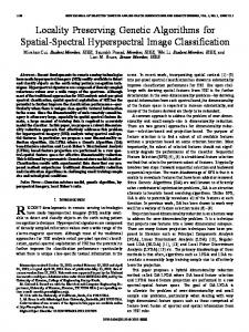
A synthetic two-dimensional aquifer is presented to demonstrate the efficiency and effectiveness of the BMcMC method. Figure 2(A) shows the spatial distribution of the reference 16 × 16 [cells] lnK field generated by LUSIM (Deutsch and Journel, 1998), having a multiGaussian characteristic. The mean and standard deviation of the lnK are set to zero and one [md−1 ], respectively. The spatial correlation structure is specified as an exponential function with a correlation length λx equal to 16 [cells], which means that the field is highly correlated. An obvious pattern of the lnK distribution is that the lower values, mainly located near the left-lower corner, are spread along the north-west direction while the higher values are mostly located around the right-lower corner and the left-upper corner. An assumed steady flow experiment is performed on this aquifer. The left and right boundary conditions are set as a prescribed head with fixed values equal to ten and zero [m], respectively. Both the upper and the lower bounds are set as non-flow. A block-centered finite-difference method is employed to solve the flow problem and the resulting head field is shown in the Figure 2(C). Nine head observations as the conditioning data set of state variables are sampled from the head field as shown in Figure 2(D). Nine lnK observations as hard data to be conditioned are also sampled from the lnK field at the same locations as head data, which are shown in Figure 2(B).

3.2

An inverse-conditioning experiment

The objective of the inverse-conditional simulation is to generate i.i.d realizations inverseconditional to the nine head samples using the proposed BMcMC method. Assume that the flow boundary conditions and the mean and covariance of lnK are correctly observed, i.e. µ = 0, σx2 = 1.0, and λx = λx = λy = 16 [cells]. The relative measurement error of state variables is set as 0.1, i.e. σy2 = 0.1. Figure 3 shows a typical BMcMC realization of lnK and the corresponding head field. Both fields reveal some of main patterns of reference models. Figure 4 shows the most probable estimate which is obtained by averaging over 3000 BMcMC realizations. The estimated lnK distribution shown in Figure 4(A) well matches the distribution of the reference lnK field: the lower values, mainly locating at the left-lower corner, spread along the north-west direction while the higher values locate mainly at the right-lower corner, although the reproduction of the left-upper corner is not that so clear. 8

(A) lnK Field (reference)

(B) lnK Data to be Conditioned

16

16

2.0

2.0

12 1.0

North

1.0

8

0.0

0.0

-1.0

-1.0

4

-2.0

-2.0

0

0 0

East

16

0

(C) Head Field (reference)

8

12

16

(D) Head Data to be Conditioned

16

16

4

10.0

10.0

9.0

9.0

12

8.0

8.0 7.0

7.0

6.0

North

6.0

5.0

8

5.0

4.0

4.0

3.0

3.0 2.0

2.0

4

1.0

1.0 0.0

0.0

0

0 0

East

16

0

4

8

12

16

Figure 2: Conditioning data sets and reference fields: (A) reference lnK field, (B) nine hard data (lnK), (C) reference head field, and (D) nine head data. The unit of hydraulic conductivity and head is in [md−1 ] and [m], respectively.

9

(A) lnK Field (No.1135)

(B) Head Field (No.1135)

16

16

2.0

10.0 9.0 8.0

1.0 7.0

North

North

6.0 0.0

5.0 4.0 3.0

-1.0 2.0 1.0 -2.0

0.0

0

0 0

East

16

0

East

16

Figure 3: A typical BMcMC realization (A) and the simulated head field (B) from (A): The unit of hydraulic conductivity and head is in [md−1 ] and [m], respectively. The precision of such estimate is plotted in Figure 4(B). One can find that the regions close to the non-flow boundaries have the most uncertainties. The mean head field shown in Figure 4(C) reasonably reflects the main characteristics of the reference head field (Figure 2(C)). The distribution of head uncertainty as plotted in Figure 4(D) also demonstrates that the regions near the non-flow boundaries have the most uncertainties. The realizations generated closely follow the prior configuration for model parameters. For example, the experimental mean and variance of the lnK are -0.13 and 0.98, respectively (Figure 5(A)), which approximate to the corresponding prior specifications, i.e. µ = 0 and σx2 = 1, and those of the reference field, i.e. µ = −0.05 and σx2 = 0.84. Figure 5 shows that the lnK distribution obeys on the Gaussian assumption and the squared head mismatch follows the log-Gaussian assumption as implied in Equation (2)-(3). In summary, head observations may contain important information for the identification of conductivity distribution. The BMcMC scheme is effective in performing stochastic simulation inverse-conditioning to head observations.

3.3

Factors that affect the performance of BMcMC

Two important factors are considered in this section to examine their influences on the performance of the BMcMC method: the correlation length (λx ) and whether or not conditioning on the hard data (x|x1 ). Several performance measures considered in this study include the reproduction of reference models, the acceptance rate, and the mixing of Markov chain. Four scenarios of BMcMC simulations with distinct configurations are run on the basis of the same conditioning data set as above. The most probable estimates are plotted in Figure 6. Compared to the larger prior correlation length (Figure 6(A) and (C)), the magnitude of 10

(A) lnK Field (ensemble mean)

(B) lnK Field (ensemble variance)

16

16

1.0

North

North

1.0

0.0

0.5

-1.0

0.0

0

0 0

East

16

0

(C) Head Field (ensemble mean)

East

16

(D) Head Field (ensemble variance)

16

16

1.0

10.0 9.0 8.0 7.0

North

North

6.0 5.0

0.5

4.0 3.0 2.0 1.0 0.0

0.0

0

0 0

East

16

0

East

16

Figure 4: A BMcMC estimate by inverse-conditioning to head observations: the simulated mean lnK field (A) and its variance (B), the simulated mean head field (C) and its variance (D). The unit of hydraulic conductivity and head is in [md−1 ] and [m], respectively.

11

(A) lnK Distribution

(B) Squared Head Misfit # of Data 16x16x3000

0.12

# of Data 3000

mean -0.13 std. dev. 0.98 coef. of var NA

Frequency

0.08

4.52 0.52 -0.14 -0.79 -4.47

maximum upper quartile median lower quartile minimum

0.12 Frequency

maximum upper quartile median lower quartile minimum

mean 1.21 std. dev. 1.48 coef. of var 1.22

0.16

58.79 1.42 1.08 0.80 0.14

0.08

0.04 0.04

0.00

0.00 -3.0

-2.0

-1.0

0.0

1.0

2.0

3.0

0.0

lnK

1.0

2.0

3.0

4.0

Squared Head Misfit

Figure 5: ln K [md−1 ] distribution (A) and squared head [m] misfit (B) lnK is underestimated by the smaller prior correlation length for both the unconditional and the conditional cases as plotted in Figure 6(B) and (D), respectively. The identified mean lnK field for the conditional case does contain the contributions from both the kriging and inverse-conditional estimate. Figure 7 compares the effects of various BMcMC configurations on the performance of Markov chain: (A)-(D) display the sequential plots of four chains with different BMcMC configurations after the chains are convergent; (E) and (F) compare the CUSUM plots of these four chains and their hairiness indices, respectively. The BMcMC parameter configurations are marked in each figures. The mean squared head mismatch in Figure 7(A)-(D) is calculated by averaging the 3000 independent realizations. One can find that the effect of the prior correlation length is minor: in the unconditional case, the correct correlation length (λx = 16) yields a slightly better mean squared head mismatch (as shown in Figure 7(A) and (B)) but a slightly worse mixing of chain (a larger excursion size in Figure 7(E) but better hairiness indices in Figure 7(F)); in the conditional case, the shorter correlation length produces better results (from Figure 7(C) through (F)). However, conditioning to hard data has considerate influence on the performance of Markov chain. The error of mean squared head misfit obviously decreases, for example, by comparing Figure 7(C) to (A), and the chain mixes more rapidly, i.e. a smaller excursion size and a larger hairiness indices. In addition, the acceptance rate is quite sensitive to the prior correlation length and whether or not conditioning on hard data. Table 1 lists 14 scenarios of stochastic simulations and their BMcMC configurations. One can easily find that conditioning to hard data significantly enhances the acceptance rate (e.g. by comparing Scenario 9-14 to Scenario 3-8). The effect of correlation length is quite complicated: for unconditional case, a correct correlation length helps increase the acceptance rate; but for the conditional case, the correct correlation length decreases the acceptance rate.

12

(A) lnK Field (ensemble mean)

(B) lnK Field (ensemble mean)

16

16

1.0

North

North

1.0

0.0

0.0

-1.0

-1.0

0

0 0

East

16

0

(C) lnK Field (ensemble mean)

East

16

(D) lnK Field (ensemble mean) 16

2.0

2.0

1.0

1.0

North

North

16

0.0

0.0

-1.0

-1.0

-2.0

-2.0

0

0 0

East

16

0

East

16

Figure 6: Factors affecting the reproduction of reference models: (A)x|y, λx = 16, (B)x|y, λx = 4, (C)x|x1 , y, λx = 16, and (D)x|x1 , y, λx = 4

13

4

4

(A) Sequential Plot of Squared Head Misfit 2 2 (x|y: σy=0.10,λx=16, =1.21)

3

∆Η2

∆Η2

3

2

2

1

0

(B) Sequential Plot of Squared Head Misfit 2 2 (x|y: σy=0.10,λx=4, =1.39)

1

0

1000

2000

0

3000

0

McMC Iteration

4

4

(C) Sequential Plot of Squared 2Head Misfit 2 (x|x1,y: σy=0.10,λx=16, =1.07)

3000

(D) Sequential Plot of Squared2 Head Misfit 2 (x|x1,y: σy=0.10,λx=4, =1.06)

3

∆Η2

∆Η2

2000

McMC Iteration

3

2

2

1

0

1000

1

0

1000

2000

0

3000

0

McMC Iteration

3000

(F) Sequential Plot of Hairiness Σt (σ2y=0.10)

0.5

x|y: λx=16 x|y: λx=4 x|x1, y: λx=16 x|x1, y: λx=4

60

2000

McMC Iteration

(E) Sequential Plot of CUSUM σt (σ2y=0.10)

120

1000

0.4

Σt

σt

0.3 0

0.2

-60

x|y: λx=16 x|y: λx=4 x|x1, y: λx=16 x|x1, y: λx=4

0.1

-120

0

1000

2000

0

3000

McMC Iteration

0

1000

2000

3000

McMC Iteration

Figure 7: Factors affecting the performance of Markov chain: (A)-(D) show the sequential plots of four chains ((A)x|y, λx = 16, (B)x|y, λx = 4, (C)x|x1 , y, λx = 16, and (D)x|x1 , y, λx = 4); (E) and (F ) display the CUSUM plots of these four chains and their hairiness indices, respectively. 14

Table 1: Summary of stochastic simulations, BMcMC configurations and performance indices Scenario x λx σy2 α(%) h∆y 2 i Σt 1 x|− 16 2 x|x1 16 3 x|y 16 0.10 0.1273 1.21 0.256 4 x|y 16 0.05 0.0175 1.24 0.047 5 x|y 16 0.02 0.0030 2.75 0.101 6 x|y 4 0.10 0.0903 1.39 0.238 7 x|y 4 0.05 0.0106 1.34 0.072 8 x|y 4 0.02 0.0028 2.38 0.108 9 x|x1 , y 16 0.10 0.8381 1.07 0.268 10 x|x1 , y 16 0.05 0.1128 0.63 0.247 11 x|x1 , y 16 0.02 0.0082 0.64 0.049 12 x|x1 , y 4 0.10 1.4622 1.06 0.281 13 x|x1 , y 4 0.05 0.1985 0.65 0.264 14 x|x1 , y 4 0.02 0.0109 0.52 0.059

4

Uncertainty Assessment

On the basis of the synthetic example presented above, the uncertainty reduction obtained by conditioning and inverse-conditioning is assessed quantitatively in terms of several measures. Two types of uncertainties are considered in this section: model uncertainty and response uncertainty. The model uncertainty is important at the spatiotemporal scale: not only because the models generated form the basis for future performance prediction at the existing wells but also because they are helpful for risk evaluation in locating new wells. The response uncertainty directly measures the prediction ability of models at the time scale.

4.1

Model uncertainty

Although the reference model is well defined and observable in this study, we generally do not know what it is ahead in practice. A practical way is to use the ensemble average of simulated outputs instead of the real model. Two parameters are computed as the metrics of performance measure to this end, the ensemble average error (I(x)1 ) and the standard deviation of the ensemble average error (I(x)2 ), which are defined as the L1 -norm and L2 norm between the simulated models and the mean models, respectively, ¯ sim k1 = I(x)1 = kxsim − x

1 nxyz

15

nxyz −1

r −1 X 1 nX |xi,r − x¯i |, n r r=0 i=0

(16)

I(x)22

= kxsim −

¯ sim k22 x

=

nxyz −1

r −1 X 1 nX (xi,r − x¯i )2 , n r r=0 i=0

1 nxyz

(17)

where nr is the number of realizations, nxyz is the number of grid cells, xsim is the vector of ¯ sim is the ensemble average vector of simulated attribute simulated attribute values, and x values. In the synthetic example considered in this study, however, the model uncertainty can be measured by the simulated errors to validate the efficiency of the proposed method since the real model is available (e.g. Deng at al., 1993). In such case, the L1 -norm and L2 -norm between the simulated models and the real models are defined as, I(x)3 = kxsim − xref k1 =

I(x)24

= kxsim −

xref k22

=

nxyz −1

r −1 X 1 nX ref |xsim i,r − xi |, nr r=0 i=0

1 nxyz

(18)

nxyz −1

r −1 X 1 nX ref 2 (xsim i,r − xi ) , n r r=0 i=0

1 nxyz

(19)

respectively. Note that xref is the vector of reference attribute values. Obviously, the smaller I(x)3 and I(x)4 are, the closer to the real model the generated realizations are.

4.2

Uncertainty of model responses

A method to examining the effect of conditioning to head data on the uncertainty reduction of the spatial distribution of hydraulic conductivity is to examine the decrease of the L1 -norm and L2 -norm of the predicted model responses (Hoeksema and Kitanidis, 1984; Kitanidis, 1986). The four metrics for the model responses are defined, I(y)1 = kysim − y¯sim k1 = I(y)22

= kysim −

y¯sim k22

=

I(y)3 = kysim − yref k1 = I(y)24

= kysim −

yref k22

=

nxyz −1

1 nxyz

nxyz

nxyz 1 nxyz

(20)

nxyz −1

1

1

r −1 X 1 nX |yi,r − y¯i |, n r r=0 i=0

r −1 X 1 nX (yi,r − y¯i )2 , n r r=0 i=0

(21)

nxyz −1

r −1 X 1 nX sim |yi,r − yiref |, nr r=0 i=0

(22)

nxyz −1

r −1 X 1 nX sim (yi,r − yiref )2 . nr r=0 i=0

(23)

In essence, I(x)1 , I(x)2 , I(y)1 , and I(y)2 measure the degree of precision that the McMC simulations could render, that is, how narrow the confidence interval of McMC simulations is. 16

I(x)3 , I(x)4 , I(y)3 , and I(y)4 measure the degree of accuracy that the McMC simulations may attain, that is, how they are close to the true model and its response. From the standpoint of estimate and uncertainty, I(x)1 , I(x)3 , I(y)1 , and I(y)3 measure the reliability of the estimated models and their responses while I(x)2 , I(x)4 , I(y)2 , and I(y)4 measure the uncertainty of the estimates and their responses.

4.3

Results

Totally fourteen scenarios of numerical experiments (see Table 1) are carried out to systematically evaluate the uncertainty reduction obtained by conditioning the hydraulic conductivity field on lnK (hard) data and head data. Table 2 summarizes the model uncertainty reduction in terms of four model metrics, I(x)1 , I(x)2 , I(x)3 , and I(x)4 . First, one can observe that the real uncertainties indicated by I(x)1 and I(x)2 are uniformly larger than the estimated uncertainties represented by I(x)3 and I(x)4 . This indicates that the model uncertainty is always underestimated by the BMcMC simulation. However, the latter two metrics can be used as a substitute of the former two for uncertainty assessment since they completely reflect the common rules that the former two reveal. Second, as the measurement errors of state variables decrease, the model accuracy does not increase much.

σy2 0.10 0.10 0.10 0.10 0.05 0.05 0.05 0.05 0.02 0.02 0.02 0.02

Table 2: Mean absolute error and mean variance of ln K x x|x1 x|y x|x1 , y x|y I(x) λx = 16 λx = 16 λx = 16 λx = 16 λx = 4 I(x)1 1.0454 0.8089 0.8686 0.7287 0.9259 I(x)22 1.3072 1.0120 1.0839 0.9216 1.1570 I(x)3 0.7978 0.6205 0.6930 0.4838 0.7525 I(x)24 0.9992 0.7929 0.8690 0.6238 0.9439 I(x)1 1.0454 0.8089 0.8623 0.7174 0.9222 2 I(x)2 1.3072 1.0120 1.0757 0.9072 1.1531 I(x)3 0.7978 0.6205 0.6871 0.4743 0.7517 2 I(x)4 0.9992 0.7929 0.8615 0.6119 0.9437 I(x)1 1.0454 0.8089 0.8766 0.7156 0.9375 2 1.3072 1.0120 1.0954 0.9056 1.1726 I(x)2 I(x)3 0.7978 0.6205 0.7040 0.4718 0.7648 0.9992 0.7929 0.8850 0.6095 0.9602 I(x)24 Ranking 6 2 3 1 5

x|x1 , y λx = 4 0.8684 1.1048 0.7026 0.8977 0.8631 1.0985 0.6961 0.8900 0.8583 1.0924 0.6925 0.8865 4

Third, the bottom line in Table 2 ranks the importance of BMcMC configurations on the model uncertainty reduction. Compared to the unconditional case, conditional simulations do reduce the model uncertainty. The case with a correct specification of model structure, 17

e.g. λx = 16, conditioning to lnK and inverse-conditioning to head data reduces the model uncertainty to the largest extent. Conditioning to lnK reduces the uncertainty more efficiently than inverse-conditioning to head data, which reveals that direct measurements of lnK are more effective for the model parameter estimation than indirect measurements of dependent state variables. However, a correct configuration of the spatial model, e.g. the correlation length λx , plays the most important role in the model uncertainty reduction. Due to the wrong specification of the correlation length, i.e. λx = 4, the conditional and inverse-conditional result only ranks the fourth, while the correct one ranks the first. In summary, the correct configuration for model structure plays a crucial role in model estimation. The direct measurement of parameters plays a more important role than the indirect measurement of dependent state data for the model parameter estimation. Table 3 summarizes the uncertainty reduction of model response in terms of four response metrics, I(y)1 , I(y)2 , I(y)3 , and I(y)4 . First, just as the observation for the model uncertainty, I(y)1 and I(y)2 are generally larger than I(y)3 and I(y)4 , which also shows that the response uncertainty is always underestimated by the BMcMC simulation. Second, as the measurement errors of state variables decrease, the model accuracy does not increase as much. Third, the bottom line in Table 3 ranks the importance of BMcMC configurations on uncertainty reduction of model response. Again, conditional and/or inverse-conditional simulations reduce the response uncertainty. The case that has a correct specification for model structure, conditioning to lnK and inverse-conditioning to head data reduces the response uncertainty to the largest extent. However, different from the model uncertainty, inverseconditioning to head data reduces the uncertainty more efficiently than conditioning to lnK, which indicates that indirect measurements of dependent state variables are more helpful to reduce the response uncertainty than direct measurements of lnK. Moreover, a correct configuration of the spatial covariance plays a less important role in reducing the response uncertainty. In summary, the response uncertainty is more sensitive to the measurements of model response than those of model parameters. It is worth mentioning that, even though the configurations for model parameter are not correct, the realizations generated well reproduce the crucial patterns of reference models (e.g. Figure 6 (B) and (D)) and both the model uncertainty and the response uncertainty are reduced by inverse-conditioning and/or conditioning (Table 2 and Table 3), which proves the robustness of the proposed BMcMC method.

5

Summary

Aiming at preserving spatial structure for inverse stochastic simulation, a blocking Markov chain Monte Carlo method is presented to generate i.i.d realizations which are conditional to hard data and inverse-conditional to state data. The proposal kernel for the construction of Markov chain is an appropriate (blocking) approximation to the target posterior distribution in the Bayesian framework. The generation of candidate realizations is very fast on the basis of the LU-decomposition of the covariance matrix. A numerical experiment on a synthetic 18

Table 3: Mean absolute error and mean variance of predicted head x x|x1 x|y x|x1 , y x|y x|x1 , y σy2 I(y) λx = 16 λx = 16 λx = 16 λx = 16 λx = 4 λx = 4 0.10 I(y)1 0.9220 0.4943 0.3072 0.2725 0.3583 0.3049 2 0.10 I(y)2 1.3217 0.7192 0.4347 0.3815 0.5053 0.4289 0.10 I(y)3 0.6806 0.3836 0.2524 0.2252 0.2834 0.2624 2 0.10 I(y)4 0.9516 0.5525 0.3580 0.3160 0.3992 0.3692 0.05 I(y)1 0.9220 0.4943 0.2946 0.2383 0.3446 0.2771 0.05 I(y)22 1.3217 0.7192 0.4453 0.3363 0.5054 0.3951 0.05 I(y)3 0.6806 0.3836 0.2436 0.1983 0.2825 0.2393 0.05 I(y)24 0.9516 0.5525 0.3749 0.2797 0.4121 0.3400 0.02 I(y)1 0.9220 0.4943 0.3616 0.2317 0.3945 0.2621 2 0.02 I(y)2 1.3217 0.7192 0.5885 0.3425 0.5957 0.3846 0.02 I(y)3 0.6806 0.3836 0.3146 0.1923 0.3265 0.2280 2 0.02 I(y)4 0.9516 0.5525 0.5103 0.2881 0.4838 0.3327 Ranking 6 5 3 1 4 2

aquifer is carried out to demonstrate the efficiency of the proposed method in performing inverse-conditional simulation. The performance of this method is also widely evaluated based on the synthetic aquifer. Numerical experiments show that the degree of heterogeneity of aquifer, e.g. correlation length (λx ), and whether or not conditioning on the hard data (x|x1 ) may play important roles in the results of inverse-conditional simulations and also affect the performance of BMcMC itself. The model uncertainty and the response uncertainty are also assessed. Both types of uncertainties are reduced due to conditioning on hard data and/or inverse-conditioning on state data. However, their influences on the uncertainty reduction may have different weights. As for the effect of the piezometric head (state data) and the hydraulic conductivity (hard data) upon the model uncertainty of lnK, the measurement of lnK plays a major role in reducing such uncertainty compared to the head data. Conditioning to head data, however, does improve the model estimation of lnK compared to conditioning to lnK solely. This conclusion is completely consistent with the result of Dagan (1985). The measurement of head is informative on the large-scale configuration of lnK. As for the effect of the piezometric head and the hydraulic conductivity upon the prediction uncertainty of head distribution, the measurement of head plays a major role in reducing such uncertainty compared to that of lnK. Although the prediction of head is quite insensitive to local lnK values, the joint conditioning to lnK does improve the prediction of head compared to inverse-conditioning to head data solely. The local measurement of lnK does not carry too much information about the spatial trend of lnK. However, the efficiency and applicability of the proposed BMcMC method for conditional 19

and inverse-conditional simulation suffers from several shortcomings. First, the fast generation of proposal kernel is totally based on the LU-decomposition of the covariance matrix which makes it very limited in dealing with the high-resolution cases. Second, the computation of the likelihood is extremely time-consuming since the forward simulation g(x) is CPU expensive. These two bottlenecks limit this method to the extensive application in practice for the conditional and inverse-conditional simulation. In addition, this study only shows the capability of the proposed BMcMC method conditioning on head data. Actually, the BMcMC method has a great flexibility in incorporating various data from different sources, e.g. the concentration data. An improved version of BMcMC method is expected to handle with the high-resolution case for the integration of various data. Acknowledgements A doctoral fellowship and an extra travel grant to the first author by the Universitat Polit`ecnica de Val`encia (UPV), Spain, is gratefully acknowledged.

References [1] Alabert, F., 1987. The practice of fast conditional simulations through the LU decomposition of the covariance matrix, Mathematical Geology, 19(5), 369-386. [2] Brooks, S.P., 1998. Quantitative convergence assessment for Markov chain Monte Carlo via cusums, Statistics and Computing, 8(3), 267-274. [3] Carrera, J., and S.P. Neuman, 1986. Estimation of aquifer parameters under transient and steady state conditions, 1. Maximum likelihood method incorporating prior information, Water Resources Research, 22(2), 199-210. [4] Dagan, G., 1985. Stochastic modeling of groundwater flow by unconditional and conditional probabilities: the inverse problem, Water Resources Research, 21(1), 65-72. [5] Deng, F.W., J.H. Cushman, and J.W. Delleur, 1993. Adaptive estimation of the log fluctuating conductivity from tracer data at the Cape Cod site, Water Resources Research, 29(12), 4011-4018. [6] Deutsch, C.V., and A.G. Journel, 1998. GSLIB: Geostatistical software library and user’s guide, second edition, Oxford University Press, pp369. [7] Davis, M.W., 1987. Production of conditional simulations via the LU triangular decomposition of the covariance matrix, Mathematical Geology, 19(2), 91-98. [8] Geman, S., and D. Geman, 1984. Stochastic relaxation, Gibbs distributions and the Bayesian restoration of images, IEEE transactions on Pattern Analysis and Machine Intelligence, 6(6), 721-741. 20

[9] Gomez-Hernandez, J.J., A. Sahuquillo, and J.E. Capilla, 1997. Stochastic simulation of transmissivity fields conditional to both transmissivity and piezometric data: I. Theory, Journal of Hydrology, 203, 162-174. [10] Hastings, W.K., 1970. Monte Carlo sampling methods using Markov chains and their application, Biometrika, 57(1), 97-109. [11] Hoeksema, R.J., and P.K. Kitanidis, 1984. An application of the geostatistical approach to the inverse problem in two-dimensional groundwater modeling, Water Resources Research, 20(7), 1003-1020. [12] Kitanidis, P.K., 1986. Parameter uncertainty in estimation of spatial functions: Bayesian analysis, Water Resources Research, 22(4), 499-507. [13] Kitanidis, P.K., 1996. On the geostatistical approach to the inverse problem, Advances in Water Resources, 19(6), 333-342. [14] Lin, Z.Y., 1992. On the increments of partial sums of a -mixing sequence, Theoretical Probability and its Applications, 36, 316-326. [15] Liu, J.S., 1996. Metropolized independent sampling with comparisons to rejection sampling and importance sampling, Statistics and Computing, 6(2), 113-119. [16] McLaughlin, D., and L.R. Townley, 1996. A reassessment of the groundwater inverse problem, Water Resources Research, 32(5), 1131-1161. [17] Metropolis, N., A.W. Rosenbluth, M.N. Rosenbluth, A.H. Teller, E. Teller, 1953. Equations of state calculations by fast computing machines, Journal of Chemical Physics, 21(3), 1087-1092. [18] Oliver, D.S., L.B. Cunha, and A.C. Reynolds, 1997. Markov chain Monte Carlo methods for conditioning a log-permeability field to pressure data, Mathematical Geology, 29(1), 61-91. [19] RamaRao, B.S., A.M. LaVenue, G. de Marsily, and M.G. Marietta, 1995. Pilot point methodology for automated calibration of an ensemble of conditionally simulated transmissivity fields: 1. Theory and computational experiments, Water Resources Research, 31(3), 475-493. [20] Robert, C.P., and G. Casella, 1999. Monte Carlo Statistical Methods, Springer-Verlag, New York, pp. 507. [21] Roberts, G.O., and S.K. Sahu, 1997. Updating schemes, correlation structure, blocking and parameterization for the Gibbs sampler, Journal of Royal Statistical Society B, 59(2), 291-317. 21

[22] Yu, B., and P. Mykland, 1998. Looking at Markov samplers through cusum path plots: a simple diagnostic idea, Statistics and Computing, 8(3), 275-286. [23] Zimmerman, D.A., G. de Marsily, C.A. Gotway, M.G. Marietta, C.L. Axness, R.L. Beauheim, R.L. Bras, J. Carrera, G. Dagan, P.B. Davies, D.P. Gallegos, A. Galli, J. Gomez-Hernandez, P. Grindrod, A.L. Gutjahr, P.K. Kitanidis, A.M. Lavenue, D. McLaughlin, S.P. Neuman, B.S. RamaRao, C. Ravenne, and Y. Rubin, 1998. A comparison of seven geostatistically based inverse approaches to estimate transmissivities for modeling advective transport by groundwater flow, Water Resources Research, 34(6), 1373-1413.

6

An LU-decomposition-based Sampler

The BMcMC computation needs a fast sampler to generate a large number of candidate realizations. The joint prior density of a multi-Gaussian random field is, ½ ¾ 1 1 −n − T −1 π(x) = (2π) 2 kCx k 2 exp − (x − µ) Cx (x − µ) , 2 where π(x) denotes the prior pdf of x ⊂ Rn ; n is the length of the vector x; µ ⊂ Rn is the prior mean of the random field; and Cx ⊂ Rn×n is the positive-definite covariance matrix of the vector x. Note that x may be partly observed, say, xobs ⊂ Rm , but seldom fully known, i.e. m < n. In such case, the sample is called a conditional simulation on linear hard data, i.e. x2 |x1 , where, x1 = xobs ⊂ Rm , x = (x1 , x2 )T , and x2 ⊂ Rn−m . The objective is to draw randomly i.i.d realizations from the distribution x ∼ N (µ, Cx ). The LU-decomposition algorithm is quite efficient and effective in generating a large number of realizations as required by the BMcMC computation since the LU-decomposition of the covariance matrix can be done once for all (Davis, 1987; Alabert, 1987). The simulated results are rather more precise and accurate than some of others, e.g. the sequential simulation algorithm.

6.1

Unconditional sampler

Sample Algorithm 1. Unconditional sample x ∼ N (µ, Cx ) , where x, µ ⊂ Rn , and Cx ⊂ Rn×n : (1) Cholesky decompose Cx = LLT , where L ⊂ Rn×n ; (2) Randomly draw z ∼ N (0, 1) ⊂ Rn ; (3) Calculate v = Lz ⊂ Rn ; (4) Generate an unconditional sample x = µ + v. 22

Note that the step 1 is only needed to be done once, which takes most of computational time. More realizations can be obtained by repeating from the step 2 to the step 4. The computational effort lies in the matrix-vector multiplication, i.e. Lz, as in the step 3.

6.2

Conditional sampler

The joint distribution of x = (x1 , x2 )T is, µ ¶ µµ ¶ · ¸¶ x1 µ1 C11 C12 ∼N , , x2 µ2 C21 C22 where x1 ⊂ Rm is the (normalized) conditioning dataset; x2 ⊂ Rn−m is the (normalized) conditional simulated values; C11 ⊂ Rm×m is the data-to-data covariance matrix; T C22 ⊂ R(n−m)×(n−m) is the unknowns-to-unknowns covariance matrix; and C21 = C12 is the (n−m)×m unknowns-to-data covariance matrix, C21 ⊂ R . It can be shown that the expected −1 value of x2 is µ2 + C21 C11 (x1 − µ1 ), which is known as the simple kriging estimate, and the −1 covariance matrix of x2 is C22 − C21 C11 C12 . Therefore, the conditional realizations can be −1 −1 ∗ ∗ ∗ drawn from x2 ∼ N (µ , C ), where µ = µ2 +C21 C11 (x1 −µ1 ) and C ∗ = C22 −C21 C11 C12 . The covariance matrix for all n grid nodes including m conditioning data can be decomposed into the product of a lower triangular matrix and an upper one, · ¸ · ¸ C11 C12 L11 U11 L11 U12 C= = LU = . C21 C22 L21 U11 L21 U12 + L22 U22 Therefore, L11 , L21 , and L22 can be obtained by C11 = L11 U11 , C21 = L21 U11 , and C22 = L21 U12 +L22 U22 , respectively. Note that the matrix multiplication, the matrix minus and the LU-decomposition are involved in the procedure of calculating the lower triangle matrices. A conditional realization x is obtained by the multiplication of L with a column vector z ⊂ Rn , µ ¶ · ¸µ ¶ x 1 − µ1 L11 0 z1 = Lz = , x 2 − µ2 L21 L22 z2 where the sub-vector z1 ⊂ Rm is set as z1 = L−1 11 (x1 − µ1 ) and the sub-vector z2 ⊂ Rn−m consists of the n − m independent standard normal deviates. Therefore, a conditional realization can be obtained by, x2 = µ2 + L21 z1 + L22 z2 = µ2 + L21 L−1 11 (x1 − µ1 ) + L22 z2 . Sample Algorithm 2. Conditional sample x2 |x1 , where the unknowns x2 ⊂ Rn−m and the hard data x1 ⊂ Rm , and x ∼ N (µ, Cx ), in which x = (x1 , x2 )T ⊂ Rn , µ ⊂ Rn , and Cx ⊂ Rn×n : (1) Calculate L11 ⊂ Rm×m from C11 = L11 LT11 ; 23

(2) Calculate L21 ⊂ R(n−m)×m from C21 = L21 LT11 ; (3) Calculate L22 ⊂ R(n−m)×(n−m) from C22 = L21 U12 + L22 LT22 ; n−m (4) Calculate the simple kriging field v1 = L21 L−1 ; 11 (x1 − µ1 ) ⊂ R

(5) Randomly draw z2 ∼ N (0, 1) ⊂ Rn−m ; (6) Calculate v2 = L22 z2 ⊂ Rn−m ; (7) Generate a conditional sample x2 = µ2 + v1 + v2 . Note that the step 1 through the step 4 are only needed to be done once which consumes the largest part of the computational efforts of this algorithm. More realizations can be obtained by repeating from the step 5 to the step 7. The computational effort focuses on the matrix-vector multiplication, i.e. L22 z2 , as in the step 6.

24