PrettyCLP: a Light Java Implementation for Teaching CLP Alessio Stalla1 , Davide Zanucco2 , Agostino Dovier2 , and Viviana Mascardi1 1
DISI - Univ. of Genova,
[email protected],
[email protected] 2 DIMI - Univ. of Udine,
[email protected],
[email protected]
Abstract. Recursion is nowadays taught to students since their first programming days in order to embed it deeply in their brains. However, students’ first impact on Prolog programs execution sometimes weakens their faith in recursive programming thus invalidating our initial efforts. The selection and computation rules implemented by all Prolog systems, although clearly explained in textbooks, are hard to be interiorized by students also due to the poor system debugging primitives. Problems increase in Constraint Logic Programming when unification is replaced by constraint simplification in a suitable constraint domain. In this paper, we extend PrettyProlog, a light-weight Prolog interpreter written in Java capable of system primitives for SLD tree visualization, to deal with Constraint Logic Programming over Finite Domains. The user, in particular, can select the propagation strategies (e.g. arc consistency vs bound consistency) and can view the (usually hidden) details of the constraint propagation stage.
1
Introduction
PrettyProlog was developed two years ago by a team of the University of Genova, for providing concrete answers to demands raised by Prolog novices [14]. Teaching experience demonstrated that one of the hardest concepts for Prolog students is to understand the construction and the visit strategy of the SLD tree. PrettyProlog was developed from scratch, without reusing any existing Prolog implementation, and designed to be simple, modular, and easily expandable. Research on visualization of the execution of Prolog programs has a long history (just to make some examples, [13, 7, 15], many papers collected in [6], and [9]). Nevertheless, nowadays few Prolog implementations offer a Stack Viewer and an SLD tree visualizer as graphical means for debugging. The open-source implementations that provide these facilities are even fewer. Among them, SWIProlog1 offers a debugging window showing current bindings, a diagrammatic trace of the call history, and a highlighted source code listing. No SLD tree visualization is given. On the other hand, many Java implementations of a Prolog 1
http://www.swi-prolog.org/
interpreter exist, starting from W-Prolog2 . Although at a prototypical stage, PrettyProlog presents three features that, to the best of our knowledge, cannot be found together in any other Prolog implementation: 1. it provides Stack and SLD Tree visualizers; 2. it is open source; 3. it is written in Java, and fully compliant with Java ME CDC application framework. The desirable architectural features of PrettyProlog have been exploited in the research activity described in this paper where PrettyProlog has been extended for dealing with Constraint Logic Programming on Finite Domains (briefly, CLP(FD)). As a matter of fact, experience in teaching CLP(FD) evidenced further problems for students, first of all the replacement of unification with constraint solving. The term 1 + 3 does not unify with the term 3 + 1. However, they are both considered as 4 by CLP(FD). Moreover, the constraint propagation stage is parametric on some choices. For instance, bounds consistency and arc consistency return different “results” to the constraint 2X = Y where the domain DX and DY of the variables X and Y are both the intervals 0..3 (DX = {0, 1}, DY = {0, 1, 2} in the former case, DX = {0, 1}, DY = {0, 2} in the latter case). Although different propagation techniques are studied in theory, Prolog interpreters supporting CLP(FD) usually implement only one of them, and students using different systems can be confused. Another source of confusion is introduced by some implementations of the SLD resolution with constraints that manage the ordering of literals in goals in a different way depending on whether they are constraint literals or user-defined literals. Moreover, during constraint’s solution search (if explicitly required by a labeling) an auxiliary tree named prop-labeling tree is created and visited. This tree is sometimes wrongly confused with the SLD tree. The proposed extension of PrettyProlog, called PrettyCLP, has been developed to help the new CLP programmers in a deeper understanding of what happens during the execution of a CLP(FD) program. The basic procedures for constraint propagation have been implemented in Java, either in the case of (hyper) arc consistency or in the case of (hyper) bounds consistency. A labeling built-in has also been developed for the solution’s search using a prop-labeling tree. This paper is organized in the following way: Section 2 recalls the functionalities of PrettyProlog and its implementation; Section 3 provides some background on CLP; Section 4 describes the original contribution of this paper, namely the design and implementation of PrettyCLP. In particular, it discusses PrettyCLP syntax, the supported mechanism for constraint propagation and labeling, and the output renderer. Section 5 analyzes the related work and concludes by outlining some future extensions. 2
http://waitaki.otago.ac.nz/~michael/wp/
2
2 2.1
PrettyProlog Functionalities
PrettyProlog implements a Prolog engine able to deal with basic data types (integer and real numbers, lists, strings), and offering metaprogramming facilities that, combined with the “cut” predicate, make the definition of negation as failure possible. Despite to some simplifications that were made during its design and implementation, sophisticated programs may be implemented with PrettyProlog thanks to these features. The main functionality of PrettyProlog, however, is that it allows the user to visualize how the Stack and the SLD Tree evolve during a computation made by the interpreter to solve a given goal. The SLD tree viewer panel shows the steps the PrettyProlog engine has performed as a tree. Each branch represents the selection of a clause from the theory, which can be selected in the “theory panel”, whereas leaves are either solutions or dead ends, i.e. goals that could not be solved. The substitution that was valid at a given point is shown aside the corresponding node in the tree. Also, the SLD tree shows which frames are removed from the stack as the effect of a cut, by printing them with a different font and icon.
Fig. 1. SLD Viewer.
3
Figure 1 shows the SLD tree of a Prolog program that implements a classical instance of a search problem: that of moving from a city in Romania (Arad, in our case) to Bucharest [11, Chapter 3]. We implemented a depth first search with control of cycles, as well as the auxiliary not and member predicates. Because of space constraints, we do not show here the code of the implemented “DFS with control of cycles” program. It can be found in [14], as well as in most Prolog textbooks. Besides showing what happens both to the stack and to the SLD tree (while it is built), PrettyProlog correctly visualizes the effect of a “cut” on the SLD tree. In the upper part of Figure 1 there are goals written in italic (from not(member(arad, [oradea, zerind, arad])), ... to !, fail, write(....) ). These nodes are cut after the execution of the ! in the first clause defining not, called with member(arad, [oradea, zerind, arad])) as argument. PrettyProlog SLD viewer keeps the cut goals for didactic purposes, but shows them in a different font to emphasize that they no longer belong to the tree. The system predicates supported by PrettyProlog, although limited, include simple predicates for input-output, such as write and nl. The stack viewer shows each frame pushed onto the stack. When the user clicks on a frame, its content is displayed: the goal that still had to be solved at the time the frame was pushed on the stack; the substitution that is the partial solution to such goal at this point; the clause that has been used to obtain the goal; the index from where, on backtracking, the engine will search for the next clause. When the PrettyProlog engine solves a goal step-by-step, the clause used in each resolution step is highlighted in the theory panel. 2.2
Implementation
PrettyProlog is made of several modules, each one corresponding roughly to a Java package. Modules are pretty much organized in a layered fashion, with the lower-level ones providing services to the upper-level ones. Currently implemented modules include: the Data Types Module, the Parser Module, the Engine Module, the GUI Module. – The Data Types Module includes data types that are commonly used throughout many other PrettyProlog modules. From this point of view, the Data Types Module is the lowest-level one. – The Parser Module contains the Parser class and some parser exception classes. This module lies just above the Data Types Module; its task is to read characters from a stream and produce instances of PrettyProlog data types, or throw an exception if something goes wrong. – The GUI Module includes the classes that make up the PrettyProlog GUI, including the viewers for the Stack, Theory, and SLD Tree. – The Engine Module is the main PrettyProlog module. It contains the Engine class as well as many helper classes such as Theory, Goal and Clause. This module contains also two sub-modules: EventListeners , which provides 4
classes and interfaces used to attach listeners to the Engine, the Stack, and the Theory; and Syspreds, which defines the built-in system predicates and gives the programmer the possibility to easily add new ones. The classes that make up the Engine Module are the following: Unifier. This class provides a single public method, unify(Term, Term), that returns a substitution that unifies the two terms passed as arguments, or null if they are not unifiable. This class exists as a separate class for reasons of modularity and extensibility. Clause. A clause is an object made of a Callable (the head) and a body, again a nameless callable. Theory. This class implements a list of clauses, with the usual operations for adding to, removing from, or navigating through the list. Frame. A Frame is a single piece of data that is contained in a stack. Stack. In addition to the usual stack operations, this class can register StackListeners which are notified of every change in the stack’s state. The lack of an explicit representation of the stack in many prolog implementations, and the requirement to have such a data structure for inspecting the behavior of the Prolog engine were the main motivations for building a new interpreter from scratch. Goal. A goal is a list of callables. Engine. The main class of the Engine module.
3
Constraint Logic Programming
We briefly recall here some basic notions of Constraint Logic Programming (CLP). The reader is referred to [10] for a recent survey. We mix syntax and semantics to shorten the presentation. Let us consider a first-order language hΠ, F, Vi, where Π, F, V are the sets of predicate symbols, functional symbols, and variables, respectively. The set Π is partitioned in the two sets ΠC and ΠP (Π = ΠC ∪ ΠP and ΠC ∩ ΠP = ∅). ΠC (ΠP ) is the set of constraints (resp., program defined) predicate symbols. ΠC is assumed to contain the equality symbol “=”. Similarly, F is partitioned into FC and FP . In this paper we focus on CLP on finite domains (CLP(FD)), therefore, we assume that FC contains the binary arithmetic function symbols +, −, ∗, /, mod etc. as well as a constant symbol for any integer number, and ΠC contains ≤, 2) if for all i ∈ {1, . . . , n} and for all di ∈ Di exist d1 ∈ D1 , . . . di−1 ∈ Di−1 , di+1 ∈ Di+1 , . . . , dn ∈ Dn such that [X1 /d1 , . . . , Xn /dn ] is a solution of c. As explained in [5] there are several definitions of bounds consistency in literature. We refer to the one implemented by SICStus Prolog3 , by B Prolog4 , and by SWI Prolog, just to cite a few, and and called interval consistency in [2]. 3 4
http://www.sics.se/isl/sicstuswww/site/ http://www.probp.com/
7
Let us consider a primitive constraint c on the variables X1 , . . . , Xn . c is bounds consistent (hyper bounds consistent if n > 2) if for all i ∈ {1, . . . , n} and for all di ∈ {min Di , max Di } (the two interval bounds), exist d1 ∈ min D1 .. max D1 , . . . , di−1 ∈ min Di−1 .. max Di−1 , di+1 ∈ min Di+1 .. max Di+1 , . . . , dn ∈ min Dn .. max Dn such that [X1 /d1 , . . . , Xn /dn ] is a solution of c. Going back to the example in the Introduction, the constraint 2X = Y where the domains DX = {0, 1}, DY = {0, 1, 2} is bounds consistent but not arc consistent.
4
PrettyCLP
This section introduces PrettyCLP: Section 4.1 reports the concrete syntax of the CLP part of PrettyCLP, Section 4.2 describes the procedures implemented for constraint propagation and labeling, and Section 4.3 shows how the output primitives have been modified and reports some system screenshots. 4.1
Concrete CLP syntax for PrettyCLP
Concretely, the set ΠC contains the constraint predicate symbols #= and #=, #>=, #< are accepted as a syntactic sugar for building negated constraint literals. Standard arithmetic functional symbols are allowed as well. The built-in instruction domain for assigning a finite domain to variables can be used in two ways (lists are usual Prolog lists): – domain(VARS, min, max), where VARS is a list of variables, and the domain is the interval min..max. – domain(VARS, DOMAIN): where VARS is a list of variables, and DOMAIN is a list of integer numbers. The labeling built-in has a unique argument: labeling(VARS), where VARS is a list of variables assigned to a finite domain. 4.2
Constraint Propagation and Labeling
Every finite domain variable is assigned to a domain, namely a set of points that can monotonically decrease during the computation, or increase again due to backtracking. Domains are stored in a vector of integer values (we recall that Java vectors are in fact a dynamic data structures that can be increased and decreased as needed). This is realized by modifying the class Variable within the module Data Types. More in detail, a Java constructor is changed in order to characterize a variable by a symbol. symbol is a PrettyProlog class, and a symbol can be the string naming a variable or a constant or functional symbol of FC . 8
Moreover, the class Domain is defined in the module Engine. This class stores an array (again, a Java dynamic array) with an entry for each of the variables occurring in the derivation and implements the methods for domain manipulation. Among them, we would like to point out the methods: – getDomain(Var X) that returns the (vector storing the) domain of a variable X. – domainVar(Var X, int min, int max) that initializes the domain of the variable X with the interval min..max. – updateDomain(Var X, Vector D) that replaces the current domain of the variable X with the domain array D. This method simplifies propagation and backtracking operations. The parser of Pretty Prolog has been slightly modified to be able to deal with constraint terms and atoms. The class Engine is the core of the computation. Since the SLD resolution is now coupled with constraint solving, we need to act on the class Engine. Unification is called for standard terms, constraint solving for constraint terms. The constructor that creates a new instance has been modified for dealing with the array domains. Then the method ContinueSolving is called. Its role is to either call the Constraint Solver procedure, called SolveConstraint, or the unification procedures already developed in PrettyProlog. The Constraint Solver returns a Boolean value: false can be obtained as effect of constraint propagation; if constraint propagation ends without failing it returns true. Constraint Propagation operates on both arc and bounds consistency. The procedures called by the Constraint Solver are: – Solve that receives as input a constraint and the domains of the variables in it and elaborates it on the basis of its main predicate symbol. When selected, unary constraints are used to reduce the domain of the corresponding variable and removed. Constraints with two or more variables, instead, are dealt with by: • ArcSolveConstraint, implementing arc consistency, and • BoundSolveConstraint, that implements bounds consistency. In these two procedures, one variable per time is selected, then every value in its domain is considered and a support for it is looked for in the domains of the remaining variables (but with a different rule for arc vs bounds). In the case of bounds, of course, a faster algorithm based on the bounds of the domains is employed. – SolveConstraint repeatedly applies the Solve procedures on all the constraints until a fixpoint is reached. – ExprEval computes the various expressions involved in constraints when values are assigned to variables and is used as auxiliary procedure by ArcSolve/ BoundSolveConstraint. The handling of labeling is made by a homonymous method. Variables in the argument list are selected from left to right (heuristics leftmost of other CLP(FD) systems) and smallest domain values are tried first (heuristics up).5 5
It it easy to implement other heuristics here. This will be done as future work.
9
This method also deals with backtracking, handling,choice points, and storing and retrieving intermediate constraint stores. Remark 1. As a final observation for this section, we would like to underline a typical problem in CLP implementations coming from the weak typing of constraint functional symbols and variables. In theory, terms and variables are sorted, in practice this is not true. If the two terms 1 + 3 and 3 + 1 are found within a unification they are assumed to be different even if the arguments are integer numbers and the binary symbol + ∈ FC . On the contrary the constraint 1 + 3 #= 3 + 1 is true. This is also the behavior of our interpreter, but this may lead a student, the target of PrettyCLP, to confusion. Similarly, let us assume to find the constraint atom X #< 3 and the variable X is not yet assigned to a domain. Some Prolog implementations will answer X in -inf..2, thus implicitly assuming a starting domain -inf..+inf for each finite domain variable. We have chosen a more rigid option: if the variable has been not yet associated with a domain, it cannot be used in a constraint atom. An error (a sort of type error) is returned. 4.3
Output rendering
After the parametric propagation procedures and the procedures for the labeling have been implemented, we modified the graphical applet of PrettyProlog for showing the new information. In particular: – buttons for visualizing and erasing domains have been added to the applet window; – the field Constraint can be inspected from the Stack Viewer; – two windows for inspecting Arc Consistency and Bounds Consistency based propagation have been made available to PrettyCLP users. Changes are done in the method TheoryViewer. In Figures 2 and 3 we report the rendering of the two alternative executions to a goal p(X,Y) where the predicate p is defined by the constraint: domain([X],0,2), domain([Y],0,5), Y #= 2 * X. In the current implementation, we decided to leave an unique SLD tree, while different computed answers are returned in the Arc Consistency and Bounds Consistency windows. Since Arc Consistency is more effective in reducing the domains, it can be the case that an inconsistent branch of the SLD tree is found some steps before than using bounds consistency. However, this case is extremely rare. We have preferred to leave the tree obtained using Bounds Consistency (the same computed by Standard Prolog system) only. However, the user can view what would have happened with the other propagation technique looking at the Arc Consistency window. In particular, all domains computed during the computation are included in those computed with Bounds Consistency. Sometimes they are strictly included and it may happen that one domain becomes empty 10
before arriving at the end of the tree. This choice can be changed as future work, namely, we could leave the user to select in advance (with a button) the propagation choice and report the selected computation only. In Figures 4–5 we report the execution of PrettyCLP on a Knapsack problem. The explicit labeling is required for variable W only. The computed solution is shown in the main picture (Fig 4). In the labeling case the differences between Arc and Bounds become evident. An excerpt of the executed constraint propagation is shown in Fig 5.
5
Related Work and Conclusions
Although visualization and tracing of constraint programs do not constitute a new research area, implemented systems that provide dynamic visualization and control functionalities for CLP(FD) are still few. Among the oldest ones we may mention the Oz-Explorer system by C. Schulte [12] which uses the search tree of a constraint problem as its central metaphor, and exploration and visualization of the search tree are user-driven and interactive. Within the community of constraint programming, ILOG debugger6 is a configurable tool with nice graphics capabilities. But, according to our opinion, it is not suitable for beginners (and it is not a CLP visual debugger). Similarly, CPVisu tracer7 is a module of the Java constraint solver on finite domains CHOCO, producing XML files that, once interpreted using CPViz8 , allow to see information on the tree search, the states of constraints and variables at different points of computations, and a configuration file. It is a professional tool (together with CHOCO, which is developed by a large group of people including Francois Laburthe, Narendra Jussien, Xavier Lorca, and other contributors, such as Nicolas Beldiceanu), but its scope is for debugging large programs rather than for learning CP (and, in any case, it does not deal with CLP). In [3], M. Carro and M. V. Hermenegildo address the design and implementation of visual paradigms for observing the execution of constraint logic programs, aiming at debugging, tuning and optimization, and teaching. They describe two tools, VIFID and TRIFID, exemplifying the devised depictions. In the companion paper [4] they describe the APT tool for running constraint logic programs while depicting a (modified) search tree, keeping information about the state of the variables at every moment in the execution. This information can be used to replay the execution at will, both forwards and backwards in time. The searchtree view is used as a framework onto which constraint-level visualizations can be attached. The integration of explanations in the trace structure and some ideas on how to implement the trace structure in a high-end system like SICStus are addressed by [1]. 6 7 8
http://www.cs.cornell.edu/w8/iisi/ilog/cp11/pdf/debugsolver.pdf http://www.emn.fr/z-info/choco-solver/cpvisu-tracer/index.html http://cpviz.sourceforge.net/
11
Fig. 2. PrettyCLP in action: Arc Consistency Propagation
Fig. 3. PrettyCLP in action: Bounds Consistency Propagation
12
Fig. 4. PrettyCLP in action: Knapsack main output
Fig. 5. PrettyCLP in action: Knapsack, propagation details
13
More recently, F. Fages, S. Soliman, and R. Coolen developed CLPGUI [8], a generic graphical user interface for visualizing and controlling the execution of constraint logic programs. CLPGUI is based on a client-server architecture for connecting a CLP process to a Java-based GUI process, and integrates a nonintrusive tracing and control method based on annotations in the CLP program. Arbitrary constraints and goals can be posted incrementally from the GUI in an interactive manner, and arbitrary states can be recomputed. Several generic 2D and 3D viewers of the variables and of the search tree are supported. Although definitely simpler than some of the above systems as far as the visualization of variables is concerned, PrettyCLP shows the original feature of allowing the user to select the propagation strategies (e.g. arc consistency vs bound consistency), which – to the best of our knowledge – is not supported by any other tool. As part of our close future activities we are planning to incorporate some global constraints, such as the alldifferent one, into PrettyCLP. Propagation procedures of global constraints allow to sensibly prune the search tree. This has effects on the size and on the form of the SLD tree too. Therefore, we will add buttons to enable/disable global consistency vs simple consistency so as to select one or the other search tree. Because of our teaching mission, from which the development of both PrettyProlog and PrettyCLP stemmed, we are currently facing the problem of guiding the student in his/her CLP learning activity. To this aim, we are designing a set of benchmarks for supporting self-evaluation and for helping students in identifying those aspects of CLP design and programming that they still need to better understand. This benchmark will heavily ground upon PrettyCLP as the tool that the students will be suggested to use in order to appreciate CLP not only on the stage, but also behind the scene. All the material relevant to PrettyProlog and PrettyCLP can be found at http://code.google.com/p/prettyprolog/. Acknowledgments This work is partially supported by INdAM-GNCS 2010, INdAM-GNCS 2011, and PRIN 20089M932N. We would like to thank Maurizio Martelli for the precious discussions during the design and implementation of the PrettyProlog visualizer.
References ˚gren, M., Szeredi, T., Beldiceanu, N., and Carlsson, M. Tracing and 1. A explaining execution of clp(fd) programs. In WLPE (2002), pp. 1–16. 2. Carlsson, M., Ottosson, G., and Carlson, B. An open-ended finite domain constraint solver. In Proc. Programming Languages: Implementations, Logics, and Programs (1997), vol. 1292 of LNCS, Springer, pp. 191–206.
14
3. Carro, M., and Hermenegildo, M. V. Tools for constraint visualisation: The vifid/trifid tool. In Analysis and Visualization Tools for Constraint Programming (2000), P. Deransart, M. V. Hermenegildo, and J. Maluszynski, Eds., vol. 1870 of Lecture Notes in Computer Science, Springer, pp. 253–272. 4. Carro, M., and Hermenegildo, M. V. Tools for search-tree visualisation: The apt tool. In Analysis and Visualization Tools for Constraint Programming (2000), P. Deransart, M. V. Hermenegildo, and J. Maluszynski, Eds., vol. 1870 of Lecture Notes in Computer Science, Springer, pp. 237–252. 5. Choi, C. W., Harvey, W., Lee, J. H. M., and Stuckey, P. J. Finite domain bounds consistency revisited. In Australian Conference on Artificial Intelligence (2006), vol. 4304 of LNCS, Springer, pp. 49–58. ´, M., Emde, A.-M., Kusalik, T., and Levy, J., Eds. Logic Program6. Ducasse ming Environments, ICLP’90 Preconference Workshop. 1990. ECRC Technical Report IR-LP-31-25. 7. Eisenstadt, M., and Brayshaw, M. A fine-grained account of Prolog execution for teaching and debugging. Instructional Science 19, 4/5 (1990), 407–436. 8. Fages, F., Soliman, S., and Coolen, R. Clpgui: A generic graphical user interface for constraint logic programming. Constraints 9, 4 (2004), 241–262. 9. Gavanelli, M. SLDNF-Draw: a visualisation tool of prolog operational semantics. In CILC’07, Messina (June 2007). 10. Gavanelli, M., and Rossi, F. Constraint logic programming. In A 25-Year Perspective on Logic Programming (2010), vol. 6125 of LNCS, pp. 64–86. 11. Russell, S., and Norvig, P. Artificial Intelligence: A Modern Approach, Second Edition. Prentice Hall, 2003. 12. Schulte, C. Using the oz explorer for the development of constraint programs. In LPE (1997), pp. 55–56. 13. Shinomi, H. Graphical representation and execution animation for Prolog programs. In MIV (1989), IEEE Computer Society, pp. 181–186. 14. Stalla, A., Mascardi, V., and Martelli, M. PrettyProlog: A Java Interpreter and Visualizer of Prolog Programs. In CILC’09, Ferrara (June 2009). System available at http://code.google.com/p/prettyprolog/. 15. Tamir, D. E., Ananthakrishnan, R., and Kandel, A. A visual debugger for pure Prolog. Inf. Sci. Appl. 3, 2 (1995), 127–147.
15