Primal-Dual Affine-Scaling Algorithms Fail for Semidefinite ...

PRIMAL-DUAL AFFINE-SCALING ALGORITHMS FAIL FOR SEMIDEFINITE PROGRAMMING MASAKAZU MURAMATSU AND ROBERT J. VANDERBEI

A BSTRACT. In this paper, we give an example of a semidefinite programming problem in which primal-dual affine-scaling algorithms using the HRVW/KSH/M, MT, and AHO directions fail. We prove that each of these algorithm can generate a sequence converging to a non-optimal solution, and that, for the AHO direction, even its associated continuous trajectory can converge to a non-optimal point. In contrast with these directions, we show that the primal-dual affine-scaling algorithm using the NT direction for the same semidefinite programming problem always generates a sequence converging to the optimal solution. Both primal and dual problems have interior feasible solutions, unique optimal solutions which satisfy strict complementarity, and are nondegenerate everywhere.

————

1. I NTRODUCTION We consider the standard form semidefinite programming (SDP) problem: minimize subject to

C•X Ai • X = bi ,

maximize subject to

bt u P Z+ m i=1 u i Ai = C,

i = 1, . . . , m,

X  0,

(1)

and its dual: Z  0,

(2)

where C, X, Ai belong to the space S (n) of n × n real symmetric matrices, P the operator • denotes the standard inner product in S (n), i.e., C • X := tr(C X ) = i, j Ci j X i j , and X  0 means that X is positive semidefinite. SDP bears a remarkable resemblance to LP. In fact, it is known that several interiorpoint methods for LP and their polynomial convergence analysis can be naturally extended to SDP (see Alizadeh [1], Jarre [15], Nesterov and Nemirovskii [28, 29], Vandenberghe and Boyd [38]). However, in extending primal-dual interior-point methods from LP to SDP, certain choices have to be made and the resulting search direction depends on these Date. March 4, 1998. 1991 Mathematics Subject Classification. Primary 60E05, Secondary 60C05. Key words and phrases. Semidefinite Programming, Primal-dual Interior-Point Method, Affine-Scaling Algorithm, Global Convergence Analysis. research partially supported by the NSF through grant CCR94-03789. 1

2

MASAKAZU MURAMATSU AND ROBERT J. VANDERBEI

choices. As a result, there can be several search directions for SDP corresponding to a single search direction for LP. This paper deals with primal-dual interior-point algorithms for SDP based on the following four search directions: (i) HRVW/KSH/M direction, (ii) MT direction, (iii) AHO direction, (iv) NT direction. We study a specific simple SDP problem, and for this problem carefully investigate the behavior of the sequence generated by the interior-point methods using these four directions to show how the convergence property of the algorithm varies depending on the choice of direction. There are two popular classes of interior-point methods: affine-scaling algorithm and path-following algorithm. Path-following algorithm is characterized by a parametric relaxation of the following optimality conditions for SDP: Ai • X Z+

m X

= bi ,

i = 1, . . . , m,

(3)

u i Ai

= C,

(4)

XZ

= µI,

(5)

i=1

X  0, Z  0, where µ > 0 is a barrier parameter. In such algorithm, it is necessary to specify a specific choice of µ at any iteration. The particulars vary from paper to paper, and we therefore omit them here. When µ ≡ 0 the corresponding method is called affine-scaling algorithm. Most of the existing SDP literature considers path-following algorithm. In this paper, we restrict our attention to affine-scaling algorithm. The affine-scaling algorithm was originally proposed for LP by Dikin [8], and independently rediscovered by Barnes [5], Vanderbei, Meketon and Freedman [39] and others, after Karmarkar [16] proposed the first polynomial-time interior-point method. Though polynomial-time complexity has not been proved yet for this algorithm, global convergence using so-called long steps was proved by Tsuchiya and Muramatsu [37]. This algorithm is often called the primal (or dual) affine-scaling algorithm because the algorithm is based on the primal (or dual) problem only. There is also a notion of primal-dual affine-scaling algorithm. In fact, for LP, there are two different types of primal-dual affine-scaling algorithm proposed to date; one by Monteiro, Adler and Resende [23], and the other by Jansen, Roos, and Terlaky [14]. The latter is sometimes called the Dikin-type primal-dual affinescaling algorithm. Both of these papers provide a proof of polynomial-time convergence for the respective algorithm, though the complexity of the former algorithm is much worse than the latter. All of the affine-scaling algorithms just described can be naturally extended to SDP. Faybusovich [9, 10] dealt with the SDP extension of the primal affine-scaling algorithm. Global convergence of the associated continuous trajectory was proved by Goldfarb and Scheinberg [12]. However, Muramatsu [27] gave an example for which the algorithm fails to converge to an optimal solution for any step size, showing that the primal affinescaling algorithm for SDP does not have the same global convergence property that one has for LP. For both primal-dual affine-scaling algorithms, de Klerk, Roos and Terlaky [7] proved polynomial-time convergence. However, as was mentioned before, there exist

PRIMAL-DUAL AFFINE-SCALING ALGORITHMS FAIL FOR SEMIDEFINITE PROGRAMMING

3

several different search directions in primal-dual interior-point methods for SDP, and each of the primal-dual affine-scaling algorithms studied by de Klerk, Roos and Terlaky was based on a certain specific choice of search direction. Below we discuss in detail how the various search directions arise. The primal-dual affine-scaling direction proposed by Monteiro, Adler and Resende [23] is the Newton direction for the set of optimality conditions, i.e., primal feasibility, dual feasibility and complementarity. For SDP, the optimality conditions are (3), (4) and X Z = 0.

(6)

A direct application of Newton’s method produces the following equations for 1X , 1u and 1Z (throughout this paper, we assume that the current point is primal and dual feasible):

1Z +

Ai • 1X

= 0,

1u i Ai

= 0,

(8)

= −X Z .

(9)

m X

i = 1, . . . , m,

(7)

i=1

X 1Z + 1X Z

However, due to (9), the solution of this system does not give a symmetric solution in general (actually 1Z must be symmetric by (8) but 1X is generally not symmetric). To date, several ways have been proposed to overcome this difficulty, each producing different directions in general. In this paper, we study a specific simple SDP problem, and for this problem carefully investigate the behavior of the sequence generated by the primal-dual affine-scaling algorithms using these four directions to show how the convergence property of the algorithm varies depending on the choice of direction. Now we describe the four directions we deal with in this paper. Note that the papers mentioned below deal exclusively with path-following algorithms, for which the corresponding affine-scaling algorithms can be derived by setting µ = 0. 1.1. The HRVW/KSH/M Direction. This direction is derived by using (7)–(9) as is, and then taking the symmetric part of the resulting 1X . This method to make a symmetric direction was independently proposed by Helmberg, Rendl, Vanderbei and Wolkowicz [13], Kojima, Shindoh and Hara [18], and Monteiro [21]. Polynomial-time convergence was proved for the path-following algorithms using this direction. For related work, see also the papers of Lin and Saigal [19], Potra and Sheng [32], and Zhang [40]. The HRVW/KSH/M direction is currently very popular for practical implementation because of its computational simplicity. Almost all SDP solvers have an option to use this direction, and some serious solvers (for example, Borchers [6] and Fujisawa and Kojima [11]) use this direction only. 1.2. The MT Direction. Monteiro and Tsuchiya [24] apply Newton’s method to the system obtained from (3)–(6) by replacing (6) with X 1/2 Z X 1/2 = 0. The resulting direction is guaranteed to be symmetric. It is the solution of (7), (8) and V Z X 1/2 + X 1/2 Z V + X 1/21Z X 1/2 VX

1/2

+X

1/2

V

= −X 1/2 Z X 1/2,

(10)

= 1X

(11)

4

MASAKAZU MURAMATSU AND ROBERT J. VANDERBEI

where V ∈ S (n) is an auxiliary variable. They proved polynomial-time convergence of the path-following algorithm using this direction. Recently, Monteiro and Zanjacomo [25] discussed a computational aspects of this direction, and gave some numerical experiments. 1.3. The AHO Direction. Alizadeh, Haeberly, and Overton [2] proposed symmetrizing equation (6) by rewriting it as X Z + Z X = 0,

(12)

and then applying Newton’s method to (3), (4) and (12). The resulting direction is a solution of (7), (8) and X 1Z + 1X Z + Z 1X + 1Z X = −(X Z + Z X ).

(13)

Several convergence properties including polynomial-time convergence are known for the path-following algorithm using the AHO direction. See for example the work of Kojima, Shida and Shindoh [17], Monteiro [22], and Tseng [36]. The AHO direction however, is not necessarily well-defined on the feasible region as observed by Shida, Shindoh and Kojima [33]; the linear system (7), (8), and (13) can be inconsistent for some problems. In fact, a specific example was given by Todd, Toh and T¨ut¨unc¨u [35]. On the other hand, Alizadeh, Haeberly, and Overton [4] report that the path-following algorithm using the AHO direction has empirically better convergence properties than the one using the HRVW/KSH/M direction. 1.4. The NT Direction. Nesterov and Todd [30, 31] proposed primal-dual algorithms for more general convex programming than SDP, which includes SDP as a special case. Their search direction naturally produces a symmetric direction. The direction is the solution of (7), (8) and 1X + D1Z D = −X,

(14)

D Z D = X.

(15)

where D ∈ S (n) is a unique solution of

Polynomial-time convergence of the corresponding path-following algorithm was proved in their original paper [30]. Also, see the works of Monteiro and Zhang [26], Luo, Sturm and Zhang [20], and Sturm and Zhang [34] for some convergence properties of the algorithms using the NT direction. The primal-dual affine-scaling algorithm studied by de Klerk, Roos and Terlaky [7] was based on this direction. As for numerical computation, Todd, Toh and T¨ut¨unc¨u [35] reported that the path-following algorithm using the NT direction is more robust than algorithms based on the HRVW/KSH/M and AHO directions. 1.5. Notation and Organization. The rest of this paper is organized as follows. In Section 2, we introduce the specific SDP problem we wish to study. Section 3, deals with the HRVW/KSH/M direction. We consider the long-step primaldual affine-scaling algorithm. One iteration of the long-step algorithm using search direction (1X, 1u, 1Z ) is as follows: X+ u+ Z+

= X + λα1X, ˆ = u + λα1u, ˆ = Z + λα1Z ˆ ,

where αˆ is defined by αˆ := min(α P , α D ),

(16)

PRIMAL-DUAL AFFINE-SCALING ALGORITHMS FAIL FOR SEMIDEFINITE PROGRAMMING

5

where αP

:= sup { α | X + α1X  0 } ,

αD

:= sup { α | Z + α1Z  0 } ,

and λ is a fixed constant less than 1. We prove that, for any fixed λ, there exists a region of initial points such that the long-step primal-dual affine-scaling algorithm using the HRVW/KSH/M direction converges to a non-optimal point. In Section 4, we prove the same statement as above for the MT direction by showing that the MT direction is identical to the HRVW/KSH/M direction for our example. In Section 5, we deal with the AHO direction. We consider the continuous trajectory which is a solution of the following autonomous differential equation: X˙ t u˙ t Z˙ t

= 1X (X t , u t , Z t ), = 1u(X t , u t , Z t ), = 1Z (X t , u t , Z t ).

(17) (18) (19)

We prove that the continuous trajectory of the AHO direction can converge to a nonoptimal point. In Section 6, we show that the long-step primal-dual affine-scaling algorithm using the NT direction generates a sequence converging to the optimal solution for any choice of λ. Note that this result does not mean the global convergence property of the algorithm, but a robust convergence property for the specific problem, for which the other three algorithms can fail to get its optimal solution. Section 7 provides some concluding remarks. Note that each section is fairly independent of the others and we use the same symbol (1X, 1u, 1Z ) for different directions; e.g., 1X in Section 3 refers to the HRVW/KSH/M direction, while in Section 5, it’s the AHO direction. 2. T HE SDP

EXAMPLE

The primal-dual pair of SDP problem we deal with in this paper is as follows:    1 0   •X  minimize  0 1  hPi 0 1   • X = 2, X  0,  subject to 1 0   maximize 2u     hDi 0 1 1 0 = , Z  0,  subject to Z + u 1 0 0 1

(20)

(21)

where X, Z ∈ S (2) and u ∈ R. The equality condition of the primal (20) says that the off-diagonal elements of X must be 1 for X to be feasible. Thus, putting   x 1 X= , (22) 1 y and noting that X  0 ⇔ x ≥ 0, y ≥ 0, x y ≥ 1, we see that problem (20) is equivalent to minimize subject to

x+y x ≥ 0,

whose optimal solution is (x, y) = (1, 1).

y ≥ 0,

x y ≥ 1,

(23)

6

MASAKAZU MURAMATSU AND ROBERT J. VANDERBEI

Similarly, from the equality condition of the dual (21), we see that Z can be written as follows:   1 −u Z= , (24) −u 1 and that the dual is equivalent to the following linear program: maximize subject to

2u −1 ≤ u ≤ 1,

(25)

whose optimal solution is obviously u = 1. Since we assume that the current point is primal and dual feasible in this paper, we see from (22) and (24) that each of the search directions has the following form:     1x 0 0 −1u 1X = , 1Z = . (26) 0 1y −1u 0 In the following, we put

F := { (x, y, u) | x y ≥ 1,

x > 0,

y > 0,

−1 ≤ u ≤ 1 } .

We see that X and Z with (22) and (24) are feasible if and only if (x, y, u) ∈ F , thus F is called primal-dual feasible region. We also define the interior of the feasible region:

F o := { (x, y, u) | x y > 1, x > 0, y > 0, −1 < u < 1 } . Obviously, if (x, y, u) ∈ F o , then the corresponding X and Z are feasible and positive definite. It is easy to see that (x ∗ , y ∗ , u ∗ ) = (1, 1, 1) is the unique optimal solutions of (23) and (25), hence     1 1 1 −1 ∗ ∗ ∗ (X , u , Z ) = , 1, 1 1 −1 1 is the unique optimal solutions of (20) and (21). It can also be easily seen that the optimal values of (20) and (21) coincide, that the optimal solutions satisfy strict complementarity, and that the problems are nondegenerate (see Muramatsu [27]; for degeneracy in SDP, see Alizadeh, Haeberly, and Overton [3]). In fact, this example problem was first proposed in Muramatsu [27] to prove that the primal affine-scaling algorithm fails. 3. T HE HRVW/KSH/M DIRECTION In this section, we consider the long-step primal-dual affine-scaling algorithm using the HRVW/KSH/M direction. To calculate the HRVW/KSH/M direction (1X, 1u, 1Z ) at a feasible point (X, u, Z ), we first solve the following system:   0 1 d = 0, • 1X (27) 1 0   0 1 1Z + 1u = 0, (28) 1 0 d Z = −X Z . X 1Z + 1X (29) d and 1Z have the following form: From (27) and (28), we see that 1X     1x 1w 0 −1u d= 1X , 1Z = . −1w 1y −1u 0

PRIMAL-DUAL AFFINE-SCALING ALGORITHMS FAIL FOR SEMIDEFINITE PROGRAMMING

7

d is Note that since we apply the HRVW/KSH/M-type method, we do not assume that 1X d symmetric here. Then we symmetrize 1X : 1X

d + 1X d t )/2 = (1X    1 1x 1w 1x = + −1w 1y 1w 2   1x 0 = . 0 1y

−1w 1y

 (30)

Therefore, 1X is independent of 1w. The third equation, (29), can be written componentwise as: −1u −y1u −x1u −1u

−u1w −1w +1w +u1w

+1x −u1x

−u1y +1y

= = = =

u − x, uy − 1, ux − 1, u − y.

Solving these linear equalities, we have 1u

=

1x

=

1y

=

2(1 − u 2 ) , x + y + 2u 2 − x y − x2 , x + y + 2u 2 − x y − y2 . x + y + 2u

(31) (32) (33)

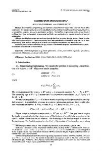
There is also an equation for 1w but we don’t write it since it disappears after symmetrization. Figure 1 shows the vector field (1x, 1y) on the primal feasible region with u = −0.5. In fact, since (1x, 1y) is independent of u after normalization, u can be arbitrary. From this figure, we can see that when x y = 1, (1x, 1y) is tangential to the boundary of the primal feasible region, and that its length is not 0 unless the current point is optimal. In the following, we will see that the primal discrete sequence (x, y) can be trapped in the curved boundary, while u remains negative. Letting the step length α(x, ˆ y, u) absorb the common factor, we can write one iteration of the primal-dual affine-scaling algorithm in terms of (x, y, u) as follows: x+

=

x + λα(x, ˆ y, u)(2 − x y − x 2 ),

(34)

+

=

y + λα(x, ˆ y, u)(2 − x y − y ),

(35)

y

u+

2

= u + 2λα(x, ˆ y, u)(1 − u 2 ),

(36)

where λ is a fixed fraction less than 1 and α(x, ˆ y, u) is defined by (16). Here, we emphasize the fact that α, ˆ which is originally a function of (X, u, Z ), can be regarded as a function of (x, y, u) due to the correspondence (22) and (24). In fact, we identify (x, y, u) and (X, u, Z ) in the following. Now we consider the set

G := { (x, y, u) ∈ F

| u ≤ 0,

1 < x y ≤ 3/2,

x + y ≥ 3 },

(37)

and investigate the property of the iteration sequence starting in this region. In fact, our aim in this section is to prove the following theorem:

8

MASAKAZU MURAMATSU AND ROBERT J. VANDERBEI

5

4.5

4

3.5

3

y 2.5

2

1.5

1

u = −0.5

0.5

0

0

0.5

1

1.5

x

F IGURE 1. Vector Field of the HRVW/KSH/M method Theorem 1. Let for any 2/3 ≤ η < 1,

Gη := { (x, y, u) ∈ G | x ≤ 1 − η } .

If, for the HRVW/KSH/M primal-dual affine-scaling algorithm (34), (35) and (36), we choose the initial point (x 0 , y 0 , u 0) ∈ G to satisfy: ! q 0 λ −u x 0 y 0 − 1 ≤ √ min , 1 − η − x0 , (38) 2 2 2 then the limit point is contained in the closure of Gη .

Since the closure of Gη does not contain the optimal solution, this theorem implies that the sequence converges to a non-optimal point. Note also that the condition (38) can be satisfied for all λ and η. In fact, fixing x 0 < 1−η and u 0 < 0, we can reduce the left hand side arbitrarily by choosing y 0 close to 1/x 0 . We first show that αˆ = α P on G . Lemma 2. If (x, y, u) ∈ G , then α(x, ˆ y, u) is a positive solution of − R(x, y)α 2 − 2(x + y)α + 1 = 0,

(39)

PRIMAL-DUAL AFFINE-SCALING ALGORITHMS FAIL FOR SEMIDEFINITE PROGRAMMING

9

where R(x, y) = on G .

(2 − x y)(x + y)2 − 4 1 ≥ >0 xy − 1 2(x y − 1)

(40)

Proof. Noting that 2(1 − u 2 ) > 0 on the interior feasible region, we have n o 1−u 1 1 = > α D = sup α u + 2α(1 − u 2) ≤ 1 = 2 2(1 − u ) 2(1 + u) 2 on G . For the primal problem (20), since x + > 0 and y + > 0 hold when x + y + ≥ 1, α P is the solution of x + y + = 1, namely, (x − α P (2 − x(x + y))) (y − α P (2 − y(x + y))) = 1. Expanding this quadratic equation and dividing by x y − 1, we have − R(x, y)α 2P − 2(x + y)α P + 1 = 0.

(41)

Now we have (40) as R(x, y) =

(2 − x y)(x + y)2 − 4 9/2 − 4 1 ≥ = >0 xy − 1 xy − 1 2(x y − 1)

on G . Since the coefficient of α 2P and the constant of (41) have the opposite signs, this quadratic equation has one positive solution and one negative, and α P is the positive solution. From (41), it follows that −2(x + y)α P + 1 = R(x, y)α 2P > 0, from which we have 1 1 ≤ ≤ αD . 2(x + y) 2 Therefore, we have αˆ = α P if (x, y) ∈ G , which is the solution of (41). αP
1 is obvious due to the choice of the step-size. Also x l+1 ≤ 1 − η ≤ 1/3 implies yl+1 ≥ 1/x l+1 ≥ 3, from which we have x l+1 +yl+1 ≥ 3. Therefore, (x l+1 , yl+1 , ul+1) ∈ Gη , which completes the proof. Remark: By replacing 3/2 with 1 +  and 3 with 2 + 2 in the definition (37) of G , the same analysis provides an initial point arbitrary close to the primal optimal solution but for which convergence is to a non-optimal point.

4. T HE MT

DIRECTION

We will show in this section that the MT direction applied with the primal and dual interchanged is identical to the HRVW/KSH/M direction for our primal-dual pair of SDP problems (20) and (21). As is well-known, we can transform the standard form SDP prob¯ h Pi ¯ of SDP lem to the dual form and vice versa to get the following primal-dual pair h Di, problems:

¯ h Di

    minimize

   subject to  maximize    ¯ h Pi subject to   



0  1 1 0

 1 •Z 0  0 • Z = 1, 0



0 0 0 1

 • Z = 1,

Z  0,

−x − y      1 0 0 0 0 1 X −x −y = , 0 1 1 0 0 0 X  0,

(42)

(43)

¯ and h Di ¯ are which is equivalent to hDi and hPi. In fact, the feasible solutions for h Pi again given by (22) and (24) where (x, y, u) ∈ F . According to (7), (8), (10) and (11), the MT direction (1X, 1x, 1y, 1Z ) for this

12

MASAKAZU MURAMATSU AND ROBERT J. VANDERBEI

primal-dual pair at a feasible solution (X, x, y, Z ) is the solution of   1 0 • 1Z = 0, 0 0   0 0 • 1Z = 0, 0 1     1 0 0 0 1X − 1x − 1y = 0, 0 0 0 1 V X Z 1/2 + Z 1/2 X V + Z 1/21X Z 1/2 VZ

1/2

+Z

1/2

V

(44) (45) (46)

= −Z 1/2 X Z 1/2

(47)

= 1Z ,

(48)

where V ∈ S (2), or equivalently, (26) and (47) and (48). The following lemma shows that the MT direction is the same as the HRVW/KSH/M direction in our problem. Lemma 6. For (X, Z ) satisfying (22) and (24) with (x, y, u) ∈ F o , the system (47), (48) d H , 1X H , 1u H , 1Z H ) be the and (26) has a unique solution (1X M , 1Z M , V M ). Let (1X solution of (26), (29), and (30) for the same (X, Z ). Then we have 1X M = 1X H and 1Z M = 1Z H . Proof. From (29) and (30), it is easy to see that 1X H is a unique solution of (X 1Z Z −1 + Z −11Z X )/2 + 1X = −X.

(49)

We prove the lemma by showing that (47) and (48) are equivalent to (49) in our case. In view of (24), we can write   cos θ sin θ , Z 1/2 = sin θ cos θ where θ satisfies cos θ > 0 and 2 cos θ sin θ = −u. Putting   p q V = , q r we have

 V Z 1/2 =

p cos θ + q sin θ q cos θ + r sin θ

p sin θ + q cos θ q sin θ + r cos θ

 .

Due to (48) and (26), the diagonal components of V Z 1/2 must be 0, i.e., p cos θ + q sin θ q sin θ + r cos θ Therefore, we have p = r, which implies that V Now we have

= 0, = 0. Z 1/2

is symmetric.

V Z 1/2 = Z 1/2 V = 1Z /2, from which V = Z −1/21Z /2 = 1Z Z −1/2/2 follow. Substituting these relations into (47), we have (Z −1/21Z X Z 1/2 + Z 1/2 X 1Z Z −1/2)/2 + Z 1/21X Z 1/2 = −Z 1/2 X Z 1/2. Obviously, (1X M , 1Z M ) is a solution of this system. Multiplying this equation by Z −1/2 from the right and left, we have (49). Since the solution of (26) and (49) is unique, the MT direction is unique and identical to the HRVW/KSH/M direction.

PRIMAL-DUAL AFFINE-SCALING ALGORITHMS FAIL FOR SEMIDEFINITE PROGRAMMING

13

The following theorem is immediate by Lemma 6. Theorem 7. Let for any 2/3 ≤ η < 1,

Gη := { (x, y, u) ∈ G | x ≤ 1 − η } .

For the long-step primal-dual affine-scaling algorithm using the MT direction, if, given a step-size parameter λ, we choose the initial point (x 0 , y 0 , u 0) ∈ G to satisfy: ! q 0 λ −u 0 x 0 y 0 − 1 ≤ √ min ,1− η − x , 2 2 2 then the limit point is contained in the closure of Gη . 5. T HE AHO

DIRECTION

We deal with the continuous trajectories of the AHO directions on our problem in this section. Let us denote the AHO direction by (1X, 1u, 1Z ). The system for the direction is (27), (28), and (13), or equivalently, (26) and (13). The third equation, (13), can be written componentwise as follows: −21u −(x + y)1u −21u

+21x −u1x

−u1y +21y

= 2(u − x), = ux + uy − 2, = 2(u − y).

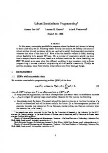
Solving these linear equalities, we have 2(1 − u 2 ) , (50) x + y + 2u 2 − x y − x 2 − u(x − y) 1x = , (51) x + y + 2u 2 − x y − y 2 − u(y − x) 1y = . (52) x + y + 2u Figure 2 shows the vector field (1x, 1y) on the primal feasible region with u = −0.5 and u = 0.5. In contrast with the HRVW/KSH/M direction case, the vector field drastically changes depending on u. Namely, when u = −0.5 and (x, y) is near the boundary of the primal feasible region, the direction is not nearly tangential to the boundary, aiming at somewhere outside of the feasible region. On the other hand when u = 0.5, the direction aims inside. The former observation leads to the convergence of the continuous trajectories of the AHO direction to a non-optimal point (Theorem 9). We deal with the trajectory (17), (18) and (19) in the space of (x, y, u) by using the oneto-one correspondence (22) and (24). Furthermore, since the trajectory is not changed if we multiply each right-hand side by a common positive factor, we can multiply by x + y + 2u which is greater than 0, to get 1u

=

x˙t

= 2 − x t yt − x t2 − u t (x t − yt ),

(53)

y˙t

= 2 − x t yt −

(54)

u˙ t

− u 2t ).

= 2(1

yt2

− u t (yt − x t ),

(55)

The equation (55) can be easily solved as follows: ut =

(1 + u 0 )e4t − (1 − u 0 ) , (1 + u 0 )e4t + (1 − u 0 )

(56)

14

MASAKAZU MURAMATSU AND ROBERT J. VANDERBEI

5

5

4.5

4.5

4

4

3.5

3.5

3

3

y 2.5

y 2.5

2

2

1.5

1.5

1

1

u = −0.5

0.5

0

0

u = 0.5

0.5

0.5

1

0

1.5

0

0.5

x

1

1.5

x

F IGURE 2. Vector Fields of the AHO method

where u 0 is the initial value of u t . The following properties of the vector field can easily be observed. Lemma 8. We have x t y˙t + yt x˙t

= u t (x t − yt )2 − 2(x t yt − 1)(x t + yt )

(57)

x t y˙t − yt x˙t

≤ u t (x t − yt ) = (x t − yt )(2 + u t (x t + yt )).

(58) (59)

2

Proof. We omit subscript t in this proof for simplicity. The former equation can be seen as: x y˙ + y x˙

= = = = ≤

x(2 − x y − y 2 − uy + ux) + y(2 − x y − x 2 − ux + uy) 2(x + y) − 2x y 2 − 2x 2 y − 2ux y + ux 2 + uy 2 2(x + y) − 2x y(x + y) + u(x − y)2 u(x − y)2 − 2(x y − 1)(x + y) u(x − y)2 .

PRIMAL-DUAL AFFINE-SCALING ALGORITHMS FAIL FOR SEMIDEFINITE PROGRAMMING

15

The latter equation can be seen as: x y˙ − y x˙

= x(2 − x y − y 2 − uy + ux) − y(2 − x y − x 2 − ux + uy) = 2x − 2y + ux 2 − uy 2 = (x − y)(2 + u(x + y)).

Now we restrict our attention to the set

H := { (x, y, u) ∈ F

| u ≤ −1/2,

y ≥ 16x } .

We then introduce the following change of variables: √ r = x y, y 1 θ = log . 2 x The inverse mapping is: x y

(60)

(61) (62)

= re−θ , = reθ .

Putting 8(x, y, u) := (r, θ, u), we can easily see that 8(H) = { (r, θ, u) | −1 ≤ u ≤ −1/2,

r ≥ 1,

θ ≥ log 4 } .

Now consider the trajectory in the new coordinate system: (rt , θt , u t ) := 8(x t , yt , u t )

(63)

starting from (r0 , θ0 , u 0 ) ∈ 8(H), and define

tˆ := sup { t > 0 | (rt , θt , u t ) ∈ 8(F ) } t¯ := sup { t > 0 | (rt , θt , u t ) ∈ 8(H) } .

ˆ u), ¯ u) We use (xˆ , yˆ , u), ˆ (ˆr , θ, ˆ (x, ¯ y¯ , u), ¯ (¯r , θ, ¯ for (x tˆ , ytˆ, u tˆ ), (rtˆ , θtˆ , u tˆ), (x t¯ , yt¯, u t¯ ), (rt¯ , θt¯ , u t¯), respectively, for notational simplicity. We will prove the following theorem in this section: Theorem 9. Let the initial point (x 0 , y0 , u 0) be in H and let (r0 , θ0 , u 0 ) = 8(x 0 , y0, u 0 ) denote the corresponding point in 8(H). If r02 − 1 < log

1 − u0 , 3(1 + u 0 )

then (x tˆ , ytˆ, u tˆ) ∈ H whereas (x ∗ , y ∗ , u ∗ ) 6∈ H.

The following lemma elucidates the behavior of the continuous trajectories on 8(H) Lemma 10. For 0 ≤ t ≤ t¯, we have rt2 θt

≤ r02 − 4t, ≤ θ0 .

(64) (65)

16

MASAKAZU MURAMATSU AND ROBERT J. VANDERBEI

Proof. It follows from (61) and (62) that r˙t

=

θ˙t

=

x t y˙t + yt x˙t 2rt x t y˙t − yt x˙t 2rt2

,

(66)

.

(67)

We have from (66) that d 2 (r ) = x t y˙t + y x˙t dt t ≤ u t (x t − yt )2 < −4

(Use (58)) (Since y − x > 3 and u ≤ 1/2 on H).

Therefore, we have rt2 − r02 < −4t. The second assertion of the lemma can be easily derived from (59) and (67), since x −y < 0 and 2 + u(x + y) ≤ 2 − (x + y)/2 < 0 on H. Now we prove the theorem. Proof of Theorem 9. Obviously, if r¯ = 1, θ¯ > log 4, and u¯ < −1/2, then the solution cannot be extended in the feasible region any more, i.e., tˆ = t¯. Since θ¯ > θ0 ≥ log 4 follows from (65), we will show that r¯ = 1 and u¯ < −1/2 in the following. Since rt ≥ 1 on 8(H), we have from (64) that t must satisfy t≤

r02 − 1 4

as far as (rt , θt , u t ) ∈ 8(H). In other words, we have t¯ ≤

r02 − 1 4


0, which implies αˆ k → 0. On the other hand, if k=1 k k k x + y − 2u → 0, then, since the optimal solution is unique, the sequence (x k , y k , u k ) converges to the optimal solution (1, 1, 1). We use these relations in the following extensively. Next lemma shows that the sequence (x k , y k , u k ) converges, and the search direction is bounded along the sequence. Lemma 13. We have (x k , y k , u k ) → (x ∞ , y ∞ , u ∞ ), and (1x k , 1y k , 1u k ) is bounded. Proof. From (77), 1u k > 0 follows. Since {u k } is an increasing sequence and bounded by 1, the limit u ∞ exists.

PRIMAL-DUAL AFFINE-SCALING ALGORITHMS FAIL FOR SEMIDEFINITE PROGRAMMING

19

We have from Lemma 12 that x k + y k ≤ x 0 + y 0 − 2u 0 + 2u k ≤ x 0 + y 0 − 2u 0 + 2, which implies that (x k , y k ) is bounded, since x k > 0 and y k > 0. By definition (78), we have φ ≥ x yρ + 1 ≥ ρ + 1 ≥ 1. Therefore, since (x k , y k , u k ) is bounded, we have |1x k | = (φ k )−1 ρ k (1 − (x k )2 ) + 2(u k − x k ) − (1 − (u k )2 )/ρ k q ρ k 1 − (x k )2 k k ≤ + 2 − x + (x k y k − 1)(1 − (u k )2 ) u 1 + (ρ k )2 q ≤ 1 − (x k )2 /2 + 2 u k − x k + (x k y k − 1)(1 − (u k )2 ) ≤

M

for some positive constant M. We see in the same way that 1y k is bounded, and, from (79), that 1u k is also bounded. If x k + y k − 2u k → 0, obviously the sequence converges to the optimal solution. Therefore, we deal with the case that x k + y k − 2u k → δˆ > 0. Then Lemma 12 implies that there exists some δ > 0 such that ∞ Y

(1 − λαˆ k ) ≥ δ.

k=0

Taking logarithm of the both sides, we have log δ ≤

∞ X

log(1 − λαˆ k ) ≤ −λ

k=0

∞ X

αˆ k .

k=0

Using this inequality, we have l X

|x k+1 − x k | ≤

k=0

l X

λαˆ k |1x k | ≤ −M log δ < ∞

k=0

for all l, which implies that {x k } is a Cauchy sequence. Thus {x k } converges. The convergence of {y k } can be shown in the same way. Using the lemma above, we prove that the dual iterates converges to its optimal. Lemma 14. We have u k → 1. Proof. Let us assume that u ∞ < 1. Since (x ∞ , y ∞ , u ∞ ) cannot be an interior point, we have x k y k → 1. If αˆ k = α kD occurs infinitely many times, then obviously u k → 1, which contradicts the assumption. Thus we can assume that α kP = αˆ k for sufficiently large k and that α kP → 0.

20

MASAKAZU MURAMATSU AND ROBERT J. VANDERBEI

On the other hand, we have α kP

= sup { α | X + α1X  0 } n o = sup α D −1 X D −1 + α D −11X D −1  0 = sup { α | Z + α(−Z − 1Z )  0 }     1−α −(1 − α)u + α1u = sup α 0 −(1 − α)u + α1u 1−α n o = sup α α ≤ 1, (1 − α)2 − ((1 − α)u − α1u)2 ≥ 0 .

Therefore, α kP satisfies (1 − α kP )2 − ((1 − α kP )u k − α kP 1u k )2 = 0.

(80)

Since 1u k is bounded, we have α kP 1u k → 0, which implies that the left hand side of (80) converges to 1 − (u ∞ )2 > 0, while the right hand side is 0. This is a contradiction, and we have u ∞ = 1. Now we know that u k → 1, and (x k , y k ) is converging. We will prove (x k , y k ) → (1, 1) in the following. To show this, we first show that the limit point is on the boundary of the primal feasible region. Lemma 15. We have x ∞ y ∞ = 1. Proof. Assume that x ∞ y ∞ = 1 + δ > 1. In this case, we have ρ k → 0 and φ k → 2 from definitions (71) and (78), and also αˆ k → 0 from Lemma 12. Since α kD

= =

1 − uk (1 − u k )φ k = k 2 k 2 k 1u (ρ ) (σ ) φ k (x k y k − 1)   p (1 + u k ) x k + y k − 2u k + 2 (1 − (u k )2 )(x k y k − 1)

→ δ/(x ∞ + y ∞ − 2) > 0, we see that α kP = αˆ k for sufficiently large k and that α kP → 0. For α kP , we have α kP

= sup { α | X + α1X  0 }   k   x + α1x k 1 = sup α 0 1 y k + α1y k n o = sup α (x k + α1x k )(y k + α1y k ) ≥ 1 n o = sup α x k y k − 1 + α(x k 1y k + y k 1x k ) + α 21x k 1y k ≥ 0 .

Therefore, αˆ kP satisfies 1x k 1y k (α kP )2 + (x k 1y k + y k 1x k )α kP + x k y k − 1 = 0.

(81)

However, since (x , y ) and (1x , 1y ) are bounded, the left hand side of (81) goes to x ∞ y ∞ − 1 = δ > 0, while the right hand side is 0. This is a contradiction, and we have x ∞ y ∞ = 1. k

k

k

k

The following relation can be seen by a straightforward calculation.

PRIMAL-DUAL AFFINE-SCALING ALGORITHMS FAIL FOR SEMIDEFINITE PROGRAMMING

21

Lemma 16. We have (x1y + y1x)φ = 2u(x + y − 2u) − δ¯(x, y, u), ¯ where δ(x, y, u) → 0 when x y → 1 and u → 1. Proof. We have x1y + y1x    q = φ −1 x ρ(1 − y 2 ) + 2(u − y) − (1 − u 2 )(x y − 1)   q +y ρ(1 − x 2 ) + 2(u − x) − (1 − u 2 )(x y − 1)   q = φ −1 ρ(x + y)(1 − x y) + 2u(x + y) − 4x y − (x + y) (1 − u 2 )(x y − 1)  = φ −1 2u(x + y − 2u) − 4(1 − u 2) − 4(x y − 1)  q −2(x + y) (1 − u 2 )(x y − 1) . Therefore, putting

q δ¯(x, y, u) := −4(1 − u 2 ) − 4(x y − 1) − 2(x + y) (1 − u 2 )(x y − 1),

we have the lemma. Now we are ready to prove that the optimality of (x ∞ , y ∞ ). Obviously, this lemma together with Lemma 17 proves Theorem 11. Lemma 17. We have (x k , y k ) → (1, 1). Proof. It can be seen that x k+1 y k+1 − 1 x k yk − 1

(x k + λαˆ k 1x k )(y k + λαˆ k 1y k ) − 1 x k yk − 1 λαˆ k (x k 1y k + y k 1x k ) + λ2(αˆ k )2 1x k 1y k = 1+ x k yk − 1
k k k k λαˆ φ (x 1y + y k 1x k ) + λαˆ k φ k 1x k 1y k = 1+ . φ k (x k y k − 1) =

(82)

We claim that φ k 1x k 1y k is bounded. Assume by contradiction, φ k 1x k 1y k is not bounded. Then we can take a diverging subsequence, i.e., there exists a subsequence L ⊂ {0, 1, 2, . . . } such that limk∈L φ k |1x k 1y k | → ∞. Since 1x k and 1y k are bounded, we have limk∈L φ k → ∞, and from the definition of φ k , limk∈L ρ k → ∞, too. Therefore this is a contradiction because, for k ∈ L,

(ρ k + u k )2 − (ρ k x k + 1)2 (ρ k + u k )2 − (ρ k y k + 1)2 k k k φ 1x 1y = (ρ k )2 φ k

(1 + u k /ρ k )2 − (x k + 1/ρ k )2 (1 + u k /ρ k )2 − (y k + 1/ρ k )2 = (y k + 1/ρ k )(x + 1/ρ k ) + (1 + u k /ρ k )2 ∞ → (1 − x )(1 − y ∞ )/2.

22

MASAKAZU MURAMATSU AND ROBERT J. VANDERBEI

Assume that (x k , y k ) 6→ (1, 1). Then Lemma 12 implies that αˆ k → 0. From Lemmas 14, 15, and 16, we have that (x k 1y k + y k 1x k )φ k ≥ x ∞ + y ∞ − 2 > 0

(83)

for sufficiently large k, while, since φ k 1x k 1y k is bounded and αˆ k → 0, αˆ k φ k 1x k 1y k → 0. Therefore, (x k 1y k + y k 1x k )φ k + λαˆ k φ k 1x k 1y k > 0 holds for sufficiently large k. This and (82) imply that x k+1 y k+1 − 1 > x k y k − 1 i.e., x k y k − 1 is increasing for sufficiently large k. This contradicts the fact that x k y k → 1. Therefore, we have (x k , y k ) → (1, 1). 7. C ONCLUDING R EMARKS The practical success of interior-point methods for LP relies heavily on the ability to take the long steps, i.e., stepping a fixed fraction of the way to the boundary for the next iterate. Even when convergence has not been proved, it is necessary in practice to take such a long step. For LP, these long steps are very successful, and every implementation uses bold step-length parameters. These bold choices of step-length parameters are supported by the robustness of the primal-dual affine-scaling algorithm (not the Dikin-type variant). It is known that the continuous trajectories associated with the primal-dual affine-scaling algorithm converge to the optimal solution, and there is no evidence so far that the long-step primal-dual affinescaling algorithm fails to find the optimal solution. However in SDP, the situation is different; even a continuous trajectory can converge to a non-optimal point. The results of this paper suggest that, for finding the optimal solution, such bold steps as are taken in the LP case should not be taken at least for the HRVW/KSH/M, MT and AHO directions; otherwise, jamming may occur. It seems that the algorithm corresponding to the NT direction is more robust than those corresponding to the other directions. The same observation was reported by Todd, Toh and T¨ut¨unc¨u [35]. ACKNOWLEDGEMENTS We thank Professor Michael Overton of New York University for showing us the bad local behavior of the HRVW/KSH/M method, which motivated us to do this research. We also thank Dr. Masayuki Shida of Kanagawa University for many stimulating discussions which inspired us to develop the results for the AHO direction, and kindly pointing out that the MT direction is identical to the HRVW/KSH/M direction in our example. R EFERENCES [1] F. Alizadeh. Interior point methods in semidefinite programming with application to combinatorial optimization. SIAM Journal on Optimization, 5:13–51, 1995. [2] F. Alizadeh, J. P. A. Haeberly, and M. L. Overton. Primal-dual interior-point methods for semidefinite programming. Technical report, 1994. [3] F. Alizadeh, J. P. A. Haeberly, and M. L. Overton. Complementarity and nondegeneracy in semidefinite programming. Technical report, 1995. [4] F. Alizadeh, J. P. A. Haeberly, and M. L. Overton. Primal-dual inteior-point methods for semidefinite programming: Convergence rates, stability and numerical results. Technical report, 1995.

PRIMAL-DUAL AFFINE-SCALING ALGORITHMS FAIL FOR SEMIDEFINITE PROGRAMMING

23

[5] E.R. Barnes. A variation on Karmarkar’s algorithm for solving linear programming problems. Mathematical Programming, 36:174–182, 1986. [6] B. Borchers. CSDP, a C library for semidefinite programming. Technical report, 1997. [7] E. de Klerk, C. Roos, and T. Terlaky. Polynomial primal-dual affine scaling algorithms in semidefinite programming. Technical Report 96-42, Delft University of Technology, 1996. [8] I.I. Dikin. Iterative solution of problems of linear and quadratic programming. Doklady Akademii Nauk SSSR, 174:747–748, 1967. (Translated in: Soviet Mathematics Doklady 8(1967)674-675.). [9] L. Faybusovich. Dikin’s algorithm for matrix linear programming problems. In J. Henry and J. Pavon, editors, Lecture notes in control and information sciences 197, pages 237–247. Springer–Verlag, 1994. [10] L. Faybusovich. On a matrix generalization of affine-scaling vector fields. SIAM Journal on Matrix Analysis and Application, 16(3):886–897, 1995. [11] K. Fujisawa and M. Kojima. SDPA (semidefinite programming algorithm) user’s manual. Technical Report B-308, Tokyo Institute of Technology, 1995. [12] D. Goldfarb and K. Scheinberg. Interior point trajectories in semidefinite programming. Technical report, Dept. of IEOR, Columbia Univsersity, New York, NY, USA, 1996. [13] C. Helmberg, F. Rendl, R.J. Vanderbei, and H. Wolkowicz. An interior point method for semidefinite programming. SIAM Journal on Optimization, 6:342–361, 1996. [14] B. Jansen, C. Roos, and T. Terlaky. A polynomial primal-dual dikin-type algorithm for linear programming. Technical Report 93-36, Faculty of Technical Mathematics and Computer Science, Delft University of Technology, Delft, The Netherlands, 1993. [15] F. Jarre. An interior-point method for minimizing the maximum eigenvalue of a linear combination of matrices. SIAM Journal on Control and Optimization, 31:1360–1377, 1993. [16] N. K. Karmarkar. A new polynomial time algorithm for linear programming. Combinatorica, 4:373–395, 1984. [17] M. Kojima, M. Shida, and S. Shindoh. A predictor-correctoe interior-point algorithm for the semidefinite linear complementarity problem using Alizadeh-Haeberly-Overton search direction. Technical report, Dept. of Mathematical and Computing Sciences, Tokyo Institute of Technology 2-12-1 Oh-Okayama, Meguro-ku, Tokyo 152, Japan, 1996. [18] M. Kojima, S. Shindoh, and S. Hara. Interior point methods for the monotone semidefinite linear complementarity problem in symmetric matrices. SIAM Journal on Optimization, 7(1):86–125, 1997. [19] C-J. Lin and R. Saigal. A predictor-corrector method for semi-definite programming. Technical report, Dept. of Industrial and Operations Engineering, The University of Michigan, Ann Arbor, Michigan 48109-2177, 1995. [20] Z-Q. Luo, J. F. Sturm, and S. Zhang. Superlinear convergence of a symmetric primal-dual path-following algorithms for semidefinite programming. Technical Report 9607/A, Econometric Institute, Erasmus University, Rotterdam, The Netherlands, 1996. [21] R. D. C. Monteiro. Primal-dual path-following algorithms for semidefinite programming. Technical report, School of Industrial and System Engineering, Georgia Tech, Atlanta, GA30332, 1995. (To appear in SIAM Journal on Optimization). [22] R. D. C. Monteiro. Polynomial convergence of primal-dual algorithms for semidefinite programming based on Monteriro and Zhang family of directions. Technical report, School of Industrial and System Engineering, Georgia Tech, Atlanta, GA30332, 1996. (To appear in SIAM Journal on Optimization). [23] R. D. C. Monteiro, I. Adler, and M. G. C. Resende. A polynomial-time primal-dual affine scaling algorithm for linear and convex quadratic programming and its power series extension. Math. of Operations Research, 15:191–214, 1990. [24] R. D. C. Monteiro and T. Tsuchiya. Polynomial convergence of a new family of primal-dual algorithms for semidefinite programming. Technical report, Georgia Institute of Technology, Atlanta, Georgia, USA, 1996. [25] R. D. C. Monteiro and P. Zanjacomo. Implementation of primal-dual methods for semidefinite programming based on monteiro and tsuchiya newton directions and their variants. Technical report, Georgia Institute of Technology, Atlanta, Georgia, USA, 1997. [26] R. D. C. Monteiro and Y. Zhang. A unified analysis for a class of path-following primal-dual interior-point algorithms for semidefinite programming. Technical report, 1996. [27] M. Muramatsu. Affine scaling algorithm fails for semidefinite programming. Technical Report 16, Department of Mechanical Engineering, Sophia University, 1996. [28] Y. E. Nesterov and A. S. Nemirovskii. Optimization over positive semidefinite matrices: Mathematical background and user’s manual. Technical report, Central Economic & Mathematical Institute, USSR Acad. Sci. Moscow, USSR, 1990.

24

MASAKAZU MURAMATSU AND ROBERT J. VANDERBEI

[29] Y. E. Nesterov and A. S. Nemirovskii. Interior Point Polynomial Methods in Convex Programming : Theory and Algorithms. SIAM Publications, Philadelphia, 1993. [30] Y. E. Nesterov and M. J. Todd. Primal-dual interior-point methods for self-scaled cones. Technical Report 1125, School of Operations Research and Industrial Engineering, Cornell University, Ithaca, New York, 14853-3801, 1995. [31] Y. E. Nesterov and M. J. Todd. Self-scaled barriers and interior-point methods for convex programming. Technical Report 1091, School of Operations Research and Industrial Engineering, Cornell University, Ithaca, New York, 14853-3801, 1995. [32] F. A. Potra and R. Sheng. A superlinearly convergent primal-dual infeasible-interior-point algorithm for semidefinite programming. Technical Report 78, Department of Mathematics, The University of Iowa, 1995. [33] M. Shida, S. Shindoh, and M. Kojima. Existence of search directions in interior-point algorithms for the sdp and the monotone SDLCP. Technical report, Dept. of Mathematical and Computing Sciences, Tokyo Institute of Technology 2-12-1 Oh-Okayama, Meguro-ku, Tokyo 152, Japan, 1996. [34] J. F. Sturm and S. Zhang. Symmetric primal-dual path-following algorithms for semidefinite programming. Technical Report 9554/A, Ecometric Institute, Erasmus University Rotterdam, The Netherlands, 1995. [35] M. J. Todd, K. C. Toh, and R. H. T¨ut¨unc¨u. On the Nesterov-Todd direction in semidefinite programming. Technical report, School of Operations Research and Industrial Engineering, Cornell University, 1996. [36] P. Tseng. Analysis of infeasible path-following methods using the Alizadeh-Haeberly-Overton direction for the monotone semidefinite lcp. Technical report, Department of Mathematics, University of Washington, Seattle, Washington 98195, U.S.A., 1996. [37] T. Tsuchiya and M. Muramatsu. Global convergence of a long-step affine scaling algorithm for degenerate linear programming problems. SIAM Journal on Optimization, 5(3):525–551, 1995. [38] L. Vandenberghe and S. Boyd. Primal-dual potential reduction method for problems involving matrix inequalities. Mathematical Programming, 69:205–236, 1995. [39] R. J. Vanderbei, M. S. Meketon, and B. F. Freedman. A modification of Karmarkar’s linear programming algorithm. Algorithmica, 1:395–407, 1986. [40] Y. Zhang. On extending primal-dual interior-point algorithms from linear programming to semidefinite programming. Technical Report TR95-20, Dept. of Math/Stat, University of Maryland, Baltimore County, Baltimore, Maryland, USA, 1995. M ASAKAZU M URAMATSU , P RINCETON U NIVERSITY , P RINCETON , NJ 08544 ROBERT J. VANDERBEI , P RINCETON U NIVERSITY , P RINCETON, NJ 08544