Primer on Multiple Regression Models for Diagnostic Imaging Research

Radiology

Statistical Concepts Series Ilana F. Gareen, PhD Constantine Gatsonis, PhD

Index term: Statistical analysis Published online 10.1148/radiol.2292030324 Radiology 2003; 229:305–310 Abbreviations: FTE ⫽ full-time equivalent ICU ⫽ intensive care unit OR ⫽ odds ratio 1

From the Center for Statistical Sciences, Brown University, Box G-H, 167 Angell St, Providence, RI 02912. Received February 19, 2003; revision requested March 25; revision received May 9; accepted May 20. Supported in part by National Cancer Institute grant CA79778. Address correspondence to I.F.G. (e-mail: igareen@stat .brown.edu).

©

RSNA, 2003

Primer on Multiple Regression Models for Diagnostic Imaging Research1 This article provides an introduction to multiple regression analysis and its application in diagnostic imaging research. We begin by examining why multiple regression models are needed in the evaluation of diagnostic imaging technologies. We then examine the broad categories of available models, notably multiple linear regression models for continuous outcomes and logistic regression models for binary outcomes. The purpose of this article is to elucidate the scientific logic, meaning, and interpretation of multiple regression models by using examples from the diagnostic imaging literature. ©

RSNA, 2003

Readers of the diagnostic imaging literature increasingly encounter articles with the results of multiple regression analyses. Typically, these analyses are performed to examine the relation of an outcome and several explanatory factors for the purpose of quantifying the effect of the explanatory factors on the outcome and/or predicting the outcome. For example, multiple regression modeling is used to study which combinations of imaging features are important predictors of the presence of disease. In this article and in the statistics literature, the explanatory variables are also referred to as covariates or independent variables, and the outcome variable is also referred to as the response or dependent variable. If the outcome is represented by a continuous variable, such as cost of care, then linear regression is often used. If the outcome is a dichotomous variable, such as presence or absence of disease, then logistic regression is commonly used. These modeling techniques provide an important tool in medical research. They enhance our ability to disentangle the nature of the relation between multiple factors that affect a single outcome. In this article, we examine why investigators choose to use multiple regression methods and how analyses with these methods should be interpreted. We use examples from the radiology literature as illustrations and focus on the meaning and interpretation of these models rather than on the methods and software used for building them.

WHAT IS REGRESSION ANALYSIS? Regression analysis provides a quantitative approach to the assessment of the relation between two or more variables, one of which is considered the dependent or response variable, and the others are considered the independent or explanatory variables (also called “covariates”). The purpose of the analysis may be to estimate the effect of a covariate or to predict the value of the response on the basis of the values of the covariates. In both cases, a regression model is developed to predict the value of the response. The way in which a model is built depends on the specific research question and the nature of the data. Each regression model incorporates assumptions regarding the nature of the data. If these assumptions are incorrect, the model may be invalid, and the interpretation of the data that is based on that model may be incorrect. The process of fitting such a model involves the specification of a shape or curve for the expected value of the response and the examination of how closely the data fit this specified shape. For example, the simple linear regression model assumes a straight-line relation between the single independent variable and the expected value of the dependent variable. The slope and intercept of this straight line are estimated from the data. The fitted model can then be used to estimate the effect of the independent variable and can also be used to predict future values of the dependent variable, which correspond to specific values of the independent variable. 305

Radiology

WHY ARE MULTIPLE REGRESSION MODELS USED IN DIAGNOSTIC IMAGING? Multiple Factors of Interest Multiple regression analyses may be used by investigators to examine the impact of multiple factors (independent variables) on a single outcome of interest (dependent variable). Sunshine and Burkhardt (1), for example, assembled survey data from 87 radiology groups on practice patterns. The authors used these data to examine the relation between the number of procedures each radiologist performed per year (dependent variable) and several independent variables, including academic status of the group, annual hours worked by each full-time radiologist, group size, and the proportion of “high-productivity” procedures (Table 1). High-productivity procedures are defined by the authors as those that require more mental effort, stress, physical effort, and training than do other types of procedures. Such procedures include CT, MR, and interventional or angiographic procedures. On the basis of the results in Table 1, it appears that workload, as measured by the dependent variable, is significantly lighter in academic groups than that in non-academic groups and decreases marginally with increasing group size. In this model, it appears that workload is not associated with the other two factors, namely group size and proportion of high-productivity procedures. The authors also report that this regression model explains only a modest amount of the variability in the dependent variable and “did not yield very accurate results.” We return to the interpretation of Table 1 later in this article.

Adjustment for Potential Confounding Multiple regression techniques may also be used to adjust analyses for potential confounding factors so that the influence of these extraneous factors is quantified and removed from the evaluation of the association of interest. Extraneous or confounding factors are those that are associated with both the exposure and the outcome of interest but are not consequences of the exposure. Consider, for example, a study to compare two diagnostic procedures (independent variable) on the basis of their impact on a patient outcome (death within a fixed follow-up period in this example). A factor such as 306

䡠

Radiology

䡠

November 2003

TABLE 1 Results of Multiple Linear Regression Analysis to Examine the Number of Annual Procedures per FTE Radiologist in Diagnostic Radiology Groups Variable

Coefficient (␤)

Standard Error*

P Value

Intercept (␤0) Academic status (X 1 ) Annual hours per FTE (X 2 ) Group size (FTE) (X 3 ) Proportion of high productivity procedures (X 4 ) †

10,403 ⫺2,238 0.43 ⫺59.7

2,154 1,123 1.11 32.5

.001 .05 .70 .07

⫺4,782

11,975

.69

Note.—Adapted and reprinted, with permission, from reference 1. * Standard error of the estimated coefficient. † High-productivity procedures included computed tomography (CT) and magnetic resonance (MR) imaging, and interventional or angiographic procedures that required more mental effort, stress, physical effort, and training than did other types of procedures.

patient age may play a role in decisions about which procedure will be performed but may also be related to the outcome. In this case, age would be a potential confounder. Clearly, confounding is a major consideration in observational studies as contrasted with randomized clinical trials, because in the former, participants are not randomly assigned to one imaging modality or another. Goodman et al (2) compared results in patients evaluated for suspected pulmonary embolism with helical CT with those evaluated with ventilation-perfusion scintigraphy to determine whether there is a difference in the number of pulmonary embolisms and deaths in the 90 days following the diagnostic imaging evaluation. The population of patients evaluated with CT was more likely to have been referred from the intensive care unit (ICU) (and, hence, more likely to have severe co-morbid disease conditions), was older, and was at increased risk of pulmonary embolism due to patient immobilization and patient malignancy than were those evaluated with ventilation-perfusion scintigraphy. To adjust for these potential confounders, the authors included them as independent variables in a logistic regression analysis and evaluated the association between imaging methods and death within 90. As a result of this adjustment, the magnitude of the estimated effect of imaging on mortality, as measured by means of the OR, changed from 3.42 to 2.54. We will return to this point later in the discussion of logistic regression.

Prediction Regression models are also used to predict the value of a response variable using the explanatory variables. For example, to develop optimal imaging strategies for

patients after trauma, Blackmore et al used clinical data from trauma patients seen in the emergency room to predict the risk of cervical spine fracture (3). The authors evaluated 20 potential clinical predictors of cervical spine injury. Their final prediction model includes four of these factors: the presence of focal neurologic deficit, presence of severe head injury, cause of injury, and patient age. These independent variables predict cervical spine fracture with a high degree of accuracy (area under the receiver operating characteristic curve ⫽ 0.87) (3).

GENERAL FORM OF REGRESSION MODELS Regression models with multiple independent variables have been constructed for a variety of types of response variables, including continuous and discrete variables. A large class of such models, and the models used most commonly in the medical literature, are the so-called generalized linear models (4). In these models, a linear relation is postulated to exist between the independent variables and the expected value of the dependent variable (or some transformed value of that expected value, such as the logarithm). The observed value of the dependent variable (response) is then the sum of its expected value and an error term. Multiple regression models for continuous, binary, and other discrete dependent variables are discussed in the following sections.

MODELING OF CONTINUOUS OUTCOME DATA First, let us consider the situation in which a continuous dependent variable Gareen and Gatsonis

Radiology

and a single independent variable are available. Such would be the case, for example, if in the practice pattern data discussed earlier, only the number of annual procedures per radiologist as the dependent variable and the radiology group size as the independent variable were considered. An earlier article in this series (5) introduced the concept of a simple linear regression model in which a linear relation is assumed between the mean of the response and the independent variable. This model is represented as Yi ⫽ ␤0 ⫹ ␤1X1i ⫹ ei, where Yi is the term representing the value of the dependent variable for the ith case, X1i represents the value of the independent random variable, ␤0 represents the intercept, ␤1 represents the slope of the linear relation between the mean of the dependent and the independent variables, and ei denotes the random error term, which has a mean of zero. The expected value of the dependent variable is then equal to ␤0 ⫹ ␤1X1i, and the error term is what is left unexplained by the model. When several independent variables are considered, such as in the analysis of the practice pattern data, multiple regression models are used. For example, assume that in addition to X1, independent variables X2, . . . , Xp are to be included in the analysis. A linear multiple regression model would then be written as Yi ⫽ ␤0 ⫹ ␤1 X1i ⫹ ␤2 X2i ⫹ · · · ⫹ ␤p Xpi ⫹ ei . The parameters ␤0, ␤1, . . . , ␤p from this equation are referred to as the regression coefficients. To interpret the coefficients, again consider first the simple linear regression model. In this model, the parameter ␤0 represents the intercept, that is, the expected value of the dependent variable when the value of the independent variable is set to zero. The parameter ␤1 represents the slope of the regression line and measures the average change in the dependent variable Y that corresponds to an increase of one unit in the independent variable X1. In multiple regression, the relation between the dependent variable Y and the independent variables X1, . . . , Xp is somewhat more complex. The intercept ␤0 represents the mean value of the response when all of the independent variables are set to zero (that is, X1 ⫽ 0, X2 ⫽ 0, . . . , Xp ⫽ 0). The slopes of the independent variables in the multiple linear regression model are interpreted in the following way. The slope ␤j of the jth independent variable measures the change in the deVolume 229

䡠

Number 2

pendent variable that corresponds to an increase of one unit in Xj, if all other independent variables are held fixed (that is, the values of the other covariates do not change). For example, the results of a multiple linear regression analysis of the practice pattern data reported by Sunshine and Burkhardt (1) are shown in Table 1. From this survey of 87 radiology groups, the dependent variable Y is the number of procedures performed annually per full-time equivalent (FTE) radiologist. X1 is a dichotomous variable and an indicator of academic status (coded 1 if the group is academic or 0 if the group is non-academic). The remaining variables can be treated as approximately continuous. X2 is the number of annual hours worked by each FTE radiologist, X3 is the practice group size, and X4 is the percentage of procedures that are high productivity. Suppressing the notation for cases, this model is written as Y ⫽ ␤ 0 ⫹ ␤ 1X 1 ⫹ ␤ 2X 2 ⫹ ␤ 3X 3 ⫹ ␤ 4X 4. The terms can be substituted into this model such that it is represented as the following equation: Y ⫽ ␤0 ⫹ ␤1 (academic status) ⫹ ␤2 (annual hours per FTE) ⫹ ␤3 (group size) ⫹ ␤4 (percentage high-productivity procedures). The estimated coefficient of X1, the indicator of academic status in the regression model, is ⫺2,238 (Table 1). Because X1 takes the values of 1 (academic group) or 0 (non-academic group), this coefficient estimate implies that, if all other independent variables remain fixed, academic groups would, on an annual basis, be expected to have 2,238 procedures per FTE radiologist less than those performed in non-academic groups (the number decreases because the coefficient is a negative number). The interpretation of coefficients for continuous independent variables is similar. For example, the model estimates that, if all other independent variables were fixed, an increase of one unit in group size would correspond to an average decrease of 59.7 in the number of procedures performed annually by each FTE radiologist in a group practice. Thus, if all other independent variables remained fixed, and practice size increased by five, the number of procedures per FTE radiologist would be expected to decrease by 5 ⫻ 59.7 ⫽ 298.5, and so on. One caveat in the interpretation of coefficients is that it is not always possible to give them a direct physical interpretation. In this example, the intercept term in the model does not have a direct in-

terpretation because it corresponds to a setting of all the independent variables to zero, which would be impossible to do. It may also be argued that it is not possible to fix some of the independent variables, such as annual hours per FTE radiologist, while allowing others, such as practice size, to vary. In Table 1, the standard error for each coefficient provides a measure of the degree of statistical uncertainty about the estimate. The fitting of models to data with a lot of scatter and small sample sizes can lead to large standard errors for the estimated coefficients. The standard error can be used to construct a confidence interval (CI) for the coefficient. The P values in Table 1 correspond to tests of the null hypothesis that a particular coefficient is equal to zero (that is, the hypothesis of “no association” between the particular independent variable and the dependent variable).

MODELING OF DICHOTOMOUS OUTCOMES Logistic regression is commonly used to analyze dichotomous outcomes (dependent variable). The independent variables in these models may be continuous, categoric, or a combination of the two. For simplicity, let us assume that the dichotomous dependent variable is coded as 0 or 1. For example, a dichotomous outcome of interest is whether each patient is dead or alive at the end of the study observation period: Y ⫽ 1 if a patient died during the follow-up interval or Y ⫽ 0 if a patient was alive at the end of the follow-up interval. In the logistic model, the expected value of the response Y is equal to the probability that Y ⫽ 1, that is, the probability that an event (such as death) occurs. The form of the model, however, is more complex than that in the linear model for continuous responses. In particular, the logit of the expected value, rather than the expected value of Y, is assumed to be a linear function of the covariates. If p denotes the probability that an event will occur, the logit of p is defined as the logarithm of the odds, that is, logit p ⫽ log[p/(1 ⫺ p)]. Formally, the logistic model with multiple independent variables is written as logit p 共Y ⫽ 1兲 ⫽ ␤0 ⫹ ␤1 X1 ⫹ · · · ⫹ ␤p Xp , or, equivalently, as 关 p共Y ⫽ 1兲兴 ⫽

e ␤0⫹␤1X1⫹· · ·⫹␤pXp 1 ⫹ e ␤0⫹␤1X1⫹· · ·⫹␤pXp

Primer on Multiple Regression Models

.

䡠

307

Radiology

In the logistic model, ␤j measures the change in log-odds for Y ⫽ 1 that corresponds to an increase of one unit in Xj, if all of the other independent variables remain fixed. In contrast to the linear model for continuous responses, the corresponding change in actual odds is multiplicative. Hence, exp(␤j) measures the odds ratio (OR) that corresponds to an increase of one unit in Xj. The OR is a frequently used measure of association in the epidemiology literature and is a common way of expressing the logistic regression results (6). The OR measures the odds of an outcome in the index group compared with the odds of the same outcome in the comparison group. For example, in the study of Goodman et al (2), Y indicates whether the patient is dead (Y ⫽ 1) or alive (Y ⫽ 0) 3 months after admission for pulmonary embolism work-up. The primary independent variable of interest, diagnostic method, would be represented by X1. Potential confounders (covariates) would be represented by X2, . . . , Xp. In Table 2, X2 is an indicator that the patient was referred from an ICU, X3 is an indicator that the patient was older than 67 years, X4 is an indicator of immobilization, and X5 is an indicator of malignancy. Substitution of these covariates into this model would result in the following representation: logit P(Y ⫽ 1) ⫽ ␤0 ⫹ ␤1 (underwent CT: yes/no) ⫹ ␤2 (ICU referral: yes/no) ⫹ ␤3 (age older than 67 years: yes/no) ⫹ ␤4 (immobilization: yes/no) ⫹ ␤5 (malignancy: yes/no). For X1, the indicator of whether or not helical CT was performed, the estimate of the coefficient was 0.93. Therefore, the estimated odds of death among patients who were evaluated with helical CT compared with that among those who were evaluated with lung scintigraphy was exp(0.93) ⫽ 2.54. That is, if all other independent variables were fixed, the odds of death within 90 days for patients who underwent CT to diagnose pulmonary embolism were 2.54 times as high as the odds for patients who underwent lung scintigraphy to diagnose pulmonary embolism. Note that this value represents an OR that was “adjusted” for the presence of potential confounders. The “unadjusted” estimate (computed from data presented in reference 2) was 3.42. Because we cannot know the counterfactual occurrence (the number of patients evaluated with CT who would have died had they been evaluated with ventilationperfusion scintigraphy), we cannot say whether the adjustment was successful, and the OR is unbiased. That there is 308

䡠

Radiology

䡠

November 2003

TABLE 2 Results of Multiple Logistic Regression Analysis to Examine Death within 90 Days of Evaluation for Pulmonary Embolism Variable Underwent CT (X 1 ) Referral from intensive care unit (X 2 ) Age older than 67 years (X 3 ) Immobilization (X 4 ) Malignancy (X 5 )

Regression Coefficient (␤)

SD

Odds Ratio

95% CI

P Value

0.93

0.32

2.54

1.36, 4.80

.004

1.78 0.75 1.26 0.87

0.32 0.34 0.39 0.34

5.93 2.12 3.52 2.39

3.09, 1.12, 1.59, 1.21,

.001 .024 .002 .012

11.0 4.14 7.58 4.63

Note.—Adapted and reprinted, with permission, from reference 2.

some difference between the unadjusted OR (3.42) and the adjusted OR (2.54) provides an indication that the potential confounders controlled for in the analysis may have been confounding the association between imaging modality and death within 90 days. However, a strong association remains between imaging method and risk of death. A CI for the OR can be obtained (6). In the example, the 95% CI for the OR is (1.36, 4.80). The authors (2) report that “the patients in the CT imaging group had more than twice the odds of dying within 90 days as those in the [ventilation-perfusion] scintigraphy group.” They also noted that “the prevalence of clinically apparent pulmonary embolism after a negative helical CT scan was low (1.0%) and minimally different from that after a normal ventilation-perfusion scan (0%)” (2). Part of this association may be due to residual confounding in the analysis. In particular, it is likely that there was confounding by indication in this sample. That is, patients with a higher likelihood of dying from pulmonary embolism were referred selectively for CT. Other more sophisticated statistical techniques may be needed to adjust for this type of confounding (7). In multiple logistic regression models, the intercept ␤0 measures the baseline log-odds for Y ⫽ 1, that is, the log-odds for Y ⫽ 1 for cases in which all independent variables have a value of zero. In the pulmonary embolism example, this would correspond to the subset of patients with all independent variables set to “no,” that is, patients who did not undergo CT, were not referred from the ICU, were 67 years old or younger, were not immobilized, and did not have a malignancy. Note that if all covariates are centered by means of subtraction of the average population value, then ␤0 measures the logodds for Y ⫽ 1 for an “average” case.

POLYNOMIAL TERMS The models discussed earlier assumed a linear relation between the independent variables and the expected value of the dependent variable. If the relation is thought to follow a non-linear form, alternative models can be considered that involve transformations of the dependent and/or independent variables. Herein, we discuss transformations of the independent variables. In a simple model with a continuous dependent variable and a continuous independent variable, if the slope of the relation appears to change with the value of the independent variable X, then a polynomial in X may be used instead of a straight line. With the example from Sunshine and Burkhardt (Table 1), if the association between the average number of procedures per radiologist and group size was not linear but seemed to be parabolic in nature, with extremes in each tail, then inclusion of a term X32 might more fully describe the observed data. The addition of higher-order (ie, X3, X4) terms may also enhance model fit (8). In addition to polynomial functions, models with other non-linear functions of the independent variables are available (8).

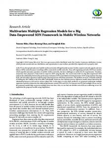
MODEL INTERPRETATION: INTERACTIONS In both linear and logistic regression, the association between the dependent variable and one of the independent variables may vary across values of another independent variable. To graphically depict this concept, the example from the Sunshine and Burkhardt article (1) is used. The relation between the number of procedures per FTE radiologist and group size for academic and nonacademic groups with no interaction terms is shown in the Figure, part a. Note that Gareen and Gatsonis

Radiology Examples of fitted regression lines of the relation between the number of procedures per FTE radiologist and group size for academic and nonacademic groups, based on the analyses presented by Sunshine and Burkhadrt (1), show (a) no statistical interaction and (b) statistical interaction.

TABLE 3 Results of Multiple Regression Analysis to Examine Coronary Restenosis Variable*

Odds Ratio

95% CI

P Value

Intercept coefficient (␤0) ⫽ 0.12 Stent use (X 1 ) Lesion length (X 2 ) PMLD (X 3 ) Previous CABG (X 4 ) Diabetes mellitus (X 5 ) Stent use ⴱ PMLD (X 6 )*

... 0.83 1.05 0.53 0.69 1.33 0.34

... 0.72, 0.97 1.04, 1.06 0.46, 0.61 0.53, 0.9 1.16, 1.54 0.31, 0.39

... .0193 ⬍.001 ⬍.001 .006 ⬍.001 .002

Source.—Reference 9. Note.—Table presents results from a multiple logistic regression analysis to examine coronary restenosis as a function of medical treatment and other selected patient characteristics. CABG ⫽ coronary artery bypass graft, PMLD ⫽ post-procedural maximum lumen diameter. * In this term, the ⴱ indicates that this is an interaction term in which stent use is multiplied by PMLD.

(diabetes mellitus) ⫹ ␤6 (stent use ⴱ PMLD). The presence of a significant interaction suggests that the effect of X1 depends on the actual level of X3 and conversely. For example, the OR for the maximal diameter size would be exp(␤3 ⫹ ␤6X1). Thus, for patients who did not receive a stent, an increase of one unit in the maximal diameter would multiply the odds of restenosis by exp(␤3). However, for patients who received a stent, the odds of restenosis would be multiplied by exp(␤3 ⫹ ␤6). Hence, in the presence of interactions, the main effects cannot be interpreted by themselves (4,6,7).

OTHER FORMS OF MULTIPLE REGRESSION MODELING the two lines, which correspond to academic and nonacademic group status, are parallel. Now, suppose that the authors want to examine whether, in fact, the two lines are parallel or not. In other words, they want to know whether the relation between the number of procedures and group size depends on academic group status. To examine this question, the authors would consider a model with an interaction term between academic group status and group size. The Figure, part b, shows how statistical interaction with another variable (academic status) might influence the relation between the number of procedures and group size. Another example is drawn from the article by Mercado et al (9). In this article, the authors examine whether placement of a stent influences the association between post-procedural minimal lumen diameter and restenosis (Table 3). Questions of this Volume 229

䡠

Number 2

type can be addressed by including appropriate “interaction” terms in the regression model. In the restenosis data, a model with an interaction between post-procedural lumen diameter and stent use can be written as follows: logit p共Y ⫽ 1兲 ⫽ ␤0 ⫹ ␤1 X1 ⫹ ␤2 X2 ⫹ ␤3 X3 ⫹ ␤4 X4 ⫹ ␤5 X5 ⫹ ␤6 X1 ⴱ X3 , where Y ⫽ 1 if restenosis occurs and 0 otherwise, X1 ⫽ stent use, X2 ⫽ lesion length, X3 ⫽ post-procedural maximum lumen diameter (PMLD), X4 ⫽ previous coronary artery bypass graft (CABG), and X5 ⫽ diabetes mellitus. X1 ⴱ X3 is a (multiplicative) interaction term between X1 and X3, in which ⴱ indicates that X1 is multiplied by X3. With the addition of the interaction term, the model would be represented as follows: logit P(Y ⫽ 1) ⫽ ␤0 ⫹ ␤1 (stent use) ⫹ ␤2 (lesion length) ⫹ ␤3 (PMLD) ⫹ ␤4 (previous CABG) ⫹ ␤5

Dependent variables that are neither continuous nor dichotomous may also be analyzed by means of specialized multiple regression techniques. Most commonly seen in the radiology literature are ordinal categoric outcomes. For example, in receiver operating characteristic studies, the radiologist’s degree of suspicion about the presence of an abnormality is often elicited on the five-point ordinal categoric scale, in which 1 ⫽ definitely no abnormality present, 2 ⫽ probably no abnormality present, 3 ⫽ equivocal, 4 ⫽ probably abnormality present, and 5 ⫽ definitely abnormality present. Ordinal regression models are available for the study of ordinal categoric outcomes. Such models can be used to fit receiver operating characteristic curves and to estimate the effect of covariates such as patient, physician, or other factors. Examples and further discussion of ordinal Primer on Multiple Regression Models

䡠

309

Radiology

regression are available in articles by Tosteson and Begg (10) and Toledano and Gatsonis (11).

RECENTERING AND RESCALING OF VARIABLES As noted earlier, in some cases an independent variable cannot possibly take the value of 0, thus making it difficult to interpret the intercept of a regression model. For example, gestational age and age at menarche cannot be meaningfully set to zero. This difficulty can be addressed by subtracting some value from the independent variable before it is used in the model. In practice, the average value of the independent variable is often used, and the “centered” form of the variable now represents the deviation from that average. When independent variables are centered at their averages, the intercept represents the expected response for an “average” case, that is, a case in which all independent variables have been set to their average values. The rescaling of variables may also enhance the interpretability of the model. Often the units in which data are presented are not those of clinical interest. By rescaling variables, each unit of increase may represent either a more clinically understandable or a more meaningful difference. For example, if gestational age is measured in days, then it may be rescaled by dividing the value for each observation by seven, which yields gestational age measured in weeks. In this case, ␤1, the regression coefficient, would then represent the difference in risk per unit increase in gestational age in weeks rather than in days.

pendent variables to include in a model is based on both subject matter and formal statistical considerations. Generally, certain independent variables will be included in the model even if they are not significantly associated with the response because they are known a priori to be related to both the exposure and the outcome of interest or to be potential confounders of the association of interest. Additional independent variables of interest are then evaluated for their contribution to an explanation of the observed variation. Models are sometimes built in a forward “stepwise” fashion in which new independent variables are added in a systematic manner, with additional terms being entered only if their contribution to the model is above a certain threshold. Alternatively, “backward elimination” may be used, starting with all potential independent variables of interest and then sequentially deleting covariates if their contribution to the model is below a fixed threshold. The validity and utility of stepwise procedures for model selection is a matter of debate and disagreement in the statistics literature (6). In addition to the selection of pertinent independent variables for inclusion in the model, it is essential to ensure that the form of the model is appropriate. A variety of regression diagnostics are available to help the analyst determine the adequacy of the postulated form of the model. Such diagnostics generally focus on examination of the residuals, which are defined as the difference between the observed and the predicted values of the response. The analyst then examines the residuals to detect the presence of patterns that suggest poor model fit (4,8).

CONCLUSION MODEL SELECTION A detailed discussion of model selection is beyond the scope of this article. We note, however, that selection of the inde-

310

䡠

Radiology

䡠

November 2003

Multiple regression models offer great utility to radiologists. These models assist radiologists in the examination of multifactorial etiologies, adjustment for multi-

ple confounding factors, and development of predictions of future outcomes. These models are adaptable to continuous, dichotomous, and other types of data, and their use may enhance the radiologist’s understanding of complex imaging utilization and clinical issues. References 1. Sunshine JH, Burkhardt JH. Radiology groups’ workload in relative value units and factors affecting it. Radiology 2000: 214:815– 822. 2. Goodman LR, Lipchik RJ, Kuzo RS, Liu Y, McAuliffe TL, O’Brien DJ. Subsequent pulmonary embolism: risk after a negative helical CT pulmonary angiogram— prosepctive comparison with scintigraphy. Radiology 2000; 215:535–542. 3. Blackmore CC, Emerson S, Mann F, Koepsell T. Cervical spine imaging in patients with trauma: determination of fracture risk to optimize use. Radiology 1999; 211:759 –765. 4. Kleinbaum DG, Kupper LL, Muller KE, Nizam A. Applied regression analysis and other multivariable methods. 3rd ed. Boston, Mass: Duxbury, 1998. 5. Zou KH, Tuncali K, Silverman SG. Correlation and simple linear regression. Radiology 2003; 227:617– 628. 6. Hosmer DW, Lemeshow S. Applied logistic regression. New York, NY: Wiley, 1989. 7. D’Agostino RB Jr. Propensity score methods for bias reduction in the comparison of a treatment to a non-randomized control group. Stat Med 1998; 17:2265–2281. 8. Neter J, Kutner M, Nachtscheim C, Wasserman W. Applied linear statistical models. 4th ed. Chicago, Ill: Irwin/McGrawHill, 1996. 9. Mercado N, Boersma E, Wijns W, et al. Clinical and quantitative coronary angiographic predictors of coronary restenosis: a comparative analysis from the balloonto-stent era. J Am Coll Cardiol 2001; 38: 645– 652. 10. Tosteson AN, Begg CB. A general regression methodology for ROC curve estimation. Med Decision Making 1988; 8:204 – 215. 11. Toledano A, Gatsonis C. Ordinal regression methodology for ROC curves derived from correlated data. Stat Med 1995 15:1807–1826.

Gareen and Gatsonis