Priority Algorithms for the Subset-Sum Problem - CiteSeerX

Priority Algorithms for the Subset-Sum Problem Yuli Ye and Allan Borodin Department of Computer Science University of Toronto Toronto, ON, Canada M5S 3G4 {y3ye,bor}@cs.toronto.edu

Abstract. Greedy algorithms are simple, but their relative power is not well understood. The priority framework [6] captures a key notion of “greediness” in the sense that it processes (in some locally optimal manner) one data item at a time, depending on and only on the current knowledge of the input. This algorithmic model provides a tool to assess the computational power and limitations of greedy algorithms, especially in terms of their approximability. In this paper, we study priority algorithm approximation ratios for the Subset-Sum Problem, focusing on the power of revocable decisions, for which the accepted data items can be later rejected to maintain the feasibility of the solution. We first provide a tight bound of α ≈ 0.657 for irrevocable priority algorithms. We then show that the approximation ratio of fixed order revocable priority algorithms is between β ≈ 0.780 and γ ≈ 0.852, and the ratio of adaptive order revocable priority algorithms is between 0.8 and δ ≈ 0.893.

1

Introduction

Greedy algorithms are of great interest because of their simplicity and efficiency. In many cases they produce reasonable (and sometimes optimal) solutions. Surprisingly, it is not obvious how to formalize the concept of a greedy algorithm and given such a formalism how to determine its power and limitations with regard to natural combinatorial optimization problems. Borodin, Nielson and Rackoff [6] suggested the priority model which provides a rigorous framework to analyze greedy-like algorithms. In this framework, they define fixed order and adaptive (order) priority algorithms, both of which capture a key notion of greedy algorithms in the sense that they process one data item at a time. For fixed order priority, the ordering function used to evaluate the priority of a data item is fixed before execution of the algorithm, while for adaptive priority, the ordering function can change during every iteration of the algorithm. By restricting algorithms to this framework, approximability results and limitations1 1

We note that similar to the study of online competitive analysis, negative priority results are in some sense incomparable with hardness of approximation results as there are no explicit complexity considerations as to how a priority algorithm can choose its next item and how it decides what to do with that item. Negative results are derived from the structure of the algorithm.

2

for many problems have been obtained; for example, scheduling problems [6, 21], facility location and set cover [1], job interval selection2 (JISP and WJISP) [15], and various graph problems [7, 10]. The original priority framework specified that decisions (being made for the current input item) are irrevocable. Even within this restrictive framework, the gap between the best known algorithm and provable negative remains significant for most problems. Following [5, 11], Horn [15] extended the priority framework to allow revocable acceptances when considering packing problems; that is, input items could be accepted and then later rejected3 , the only restriction being that a feasible solution is maintained at the end of each iteration. The revocable (decision) priority model is intuitively more powerful and almost as conceptually simple as the irrevocable model and it is perhaps surprising that it is not a more commonly used type of algorithm. Erlebach and Spieksma [11] and independently Bar-Noy et al. [5] provide a simple revocable priority approximation algorithm for the WJISP problem, and Horn [15] formalizes this model and provides an approximation upper bound4 of ≈ 1/(1.17) for the special case of the weighted interval scheduling problem. Moore’s [20] “greedy algorithm” for the throughput maximization P unweighted ¯j in Graham’s scheduling notation) problem without release times (i.e. 1|| j U solves the problem optimally, and it can also be viewed as a fixed order revocable priority algorithm. So the notion of revocable decisions has been used in the previous research, but it has not yet received much attention. The Subset-Sum Problem (SSP) is one of the most fundamental NP-complete problems [13], and perhaps the simplest of its kind. Approximation algorithms for SSP have been studied extensively in the literature. The first FPTAS (for the more general knapsack problem) is due to Ibarra and Kim [16], and the best current approximation algorithm is due to Kellerer et al. [18], having time and space complexity O(min{ nε , n+ ε12 log 1ε }) and O(n+ 1ε ) respectively. Greedy-like approximation algorithms have also been studied for SSP; an algorithm called greedy but using multiple passes, has approximation ratio 0.75, see [19]. In this paper, we study priority algorithms for SSP. Although in some sense one may consider SSP to be a “solved problem”, the problem still presents an interesting challenge for the study of greedy algorithms. We believe the ideas employed for SSP will be applicable to the study of simple algorithms for other (say scheduling) problems which are not well understood, such as the throughput maximization problem (with release times) and some of its more tractable subcases. In particular, can we derive priority approximation algorithms for throughput P max¯j )? imization when all jobs have a fixed processing time (i.e. 1|rj , pj = p| j wj U (We note that Horn’s [15] 1/(1.17) bound also applies to this problem.) Bap2

3 4

In the job interval selection problem (JISP), we are given a set of jobs with unit profit and each job consists of a set of intervals. The objective is to maximize the total profit of scheduled jobs without conflicting intervals such that there is at most one interval per job. WJISP is the weighted version of JISP. Once a data item is rejected, it cannot become part of the solution in the future. As we are considering maximization problems in this paper, all approximation ratios will be ≤ 1 so that negative results become upper bounds on the ratio.

3

tiste [4] optimally solves this special case of throughput maximization using a dynamic programming algorithm with time complexity O(n7 ). (See also Chuzhoy et al. [9] and Chrobak et al. [8] for additional throughput maximization results.) In spite of the conceptual simplicity of the SSP problem and the priority framework, there is still a great deal of flexibility in how one can design algorithms, both in terms of the ordering and in terms of which items to accept and (for the revocable model) which items to discard in order to fit in a new item. We give a tight bound of α ≈ 0.657 for irrevocable priority algorithms showing that in this case adaptive ordering does not help. For fixed order revocable algorithms, we can show that the best approximation ratio is between β ≈ 0.780 and γ ≈ 0.852; for adaptive revocable priority algorithms, the best approximation ratio is between 0.8 and δ ≈ 0.893. In some sense, one should not be surprised at the flexibility within the priority model. Indeed, even for the much more restricted class of online algorithms (where an adversary dictates the ordering), there can be (at first) non-intuitive algorithms. As an example, we remark that for Graham’s [14] classic makespan problem for identical machines, there is still an open problem as to the optimal online approximation ratio (i.e. competitive ratio). Here, one improves upon the natural greedy algorithm by not always making a greedy choice but instead saving some space for future potentially large items. (For the current best competitive ratio 1.9201, see Fleisher and Wahl [12] following a series of results 1 improving on Graham’s 2 − m bound for the greedy algorithm on m machines.) In the related and unrelated machine models, the natural greedy algorithm is not O(1) competitive and the best known competitive algorithms for these models are not at all obvious (see Aspnes, et al. [3]).

2

Definitions and Notation

We use bold font letters to denote sets of data items. For a given set R of data items, we use |R| to denote its cardinality and kRk, its total weight. For a data item u, we use u to represent the singleton set {u} and 2u, the multi-set {u, u}; we also use u to represent the weight of u since it is the only attribute. The term u here is an overloaded term, but the meaning will become clear in the actual context. For set operations, we use ⊕ to denote set addition, and use ⊖ to denote set subtraction. 2.1

The Subset-Sum Problem

Given a set of n data items with positive weights and a capacity c, the maximization version of SSP is to find a subset such that the corresponding total weight is maximized without exceeding the capacity c. Without loss of generality, we make two assumptions. First of all, the weights are all scaled to their relative values to the capacity; hence we can use 1 instead of c for the capacity. Secondly, we assume each data item has weight ∈ (0, 1]. An instance σ of SSP is a set I = {u1 , u2 , . . . , un } of n data items, where the set I is the input

4

set, and u1 , u2 , . . . , un are the data items. A feasible solution of σ is a subset B of I such that kBk ≤ 1. An optimal solution of σ is a feasible solution with maximum weight. We can formulate SSP as a solution of the following integer programming: maximize

n X

ui xi

(1)

subject to

i=1 n X

ui xi ≤ 1,

(2)

i=1

where xi ∈ {0, 1} and i ∈ [1, n]. Let A be an algorithm for SSP, for a given instance σ, we denote A(σ) the solution achieved by A and OPT(σ), the optimal solution, then the approximation ratio of A on σ is denoted by ρ(A, σ) =

kA(σ)k . kOPT(σ)k

Let Σ be the set of all instances of SSP, then the approximation ratio of A over Σ is denoted by ρ(A) = inf ρ(A, σ). σ∈Σ

In a particular analysis, the algorithm and the problem instance are usually fixed. For convenience, we often use ALG, OPT and ρ to denote the algorithm’s solution, the optimal solution and the approximation ratio respectively. 2.2

Priority Model

We base our terminology and model on that of [6], and start with the class of fixed order irrevocable priority algorithms for SSP. For a given instance, a fixed order irrevocable priority algorithm maintains a feasible solution B throughout the algorithm. The structure of the algorithm5 is as follows: Fixed Order Irrevocable Priority Ordering: Determine a total ordering of all possible data items while I is not empty next := index of the data item in I that comes first in the ordering Decision: Decide whether or not to add unext to B, and then remove unext from I end while 5

We formalize the allowable (fixed) orderings by saying that the algorithm specifies a total ordering on all possible input items. The items that constitute the actual input set I will then inherit this ordering. That is, the priority model insists that the ordering satisfies Arrow’s Independence of Irrelevant Attributes (IIA) Axiom[2]. For adaptive orderings the algorithm can construct a new IIA ordering based on all the items that it has already seen as well as those items it can deduce are not in the input set.

5

An adaptive irrevocable priority algorithm is similar to a fixed order one, but instead of looking at a data item according to some pre-determined ordering, the algorithm is allowed to reorder the remaining data items in I at each iteration. This gives the algorithm an advantage since now it can take into account the information that has been revealed so far to determine which is the best data item to consider next. The structure of an adaptive irrevocable priority algorithm is described as follows: Adaptive Irrevocable Priority while I is not empty Ordering: Determine a total ordering of all possible (remaining) data items next := index of the data item in I that comes first in the ordering Decision: Decide whether or not to add unext to B, and then remove unext from I end while The above defined priority algorithms are “irrevocable” in the sense that once a data item is admitted to the solution it cannot be removed. We can extend our notion of “fixed order” and “adaptive” to the class of revocable priority algorithms, where revocable decisions on accepted data items are allowed. Accordingly, those algorithms are called fixed order revocable and adaptive revocable priority algorithms respectively. The extension6 to revocable acceptances provides additional power; for example, as shown in [17], online irrevocable algorithms for SSP cannot achieve any constant bound approximation ratio, while online √ ≈ 0.618. revocable algorithms can achieve a tight approximation ratio of 5−1 2 2.3

Adversarial Strategy

We utilize an adversary in proving approximation bounds. For a given priority algorithm, we run the adversary against the algorithm in the following scheme. At the beginning of the algorithm, the adversary first presents a set of data items to the algorithm, possibly with some data items having the same weight. Furthermore, our adversary promises that the actual input is contained in this set7 . Since weight is the only input parameter, the algorithm give the same priority to all items having the same weight 8 . At each step, the adversary asks the algorithm to select one data item in the remaining set and make a decision on that data item. Once the algorithm makes a decision on the selected item, the adversary then has the power to remove any number of data items in the remaining set; this repeats until the remaining set is empty, which then terminates the algorithm. 6 7

8

This extension applies to priority algorithms for packing problems. This assumption is optional. The approximation bounds clearly hold for a stronger adversary. Technically we can use an item number identifier to further distinguish items, but by providing sufficiently many copies of an item the adversary can effectively achieve what the statement claims.

6

For convenience, we often use a diagram to illustrate an adversarial strategy. A diagram of an adversarial strategy is an acyclic directed graph, where each node represents a possible state of the strategy, and each arc indicates a possible transition. Each state of the strategy contains two boxes. The first box indicates the current solution maintained by the algorithm, the second box indicates the remaining set of data items maintained by the adversary. A state can be either terminal or non-terminal. A state is terminal if and only if it is a sink, in the sense that the adversary no longer need perform any additional action; we indicate a terminal state using bold boxes. Each transition also contains two lines of actions. The first line indicates the action taken by the algorithm and the second line indicates the action taken by the adversary. Sometimes the algorithm may need to reject certain data items in order to accept a new one, so an action may contain multiple operations which occur at the same time; we use ⊘ to indicate no action. Note that to calculate a bound for the approximation ratio of an algorithm, it is sufficient to consider the approximation ratios achieved in all terminal states. We will see such diagrams in Sect. 4.

3

General Simplifications

We first provide two simplifications for general priority algorithms, both of which are based on the approximation ratio, say θ, we want to achieve. 3.1

Implicit Terminal Conditions

Since we are interested in approximation algorithms, we can terminate an algorithm at any time if the approximation ratio of θ is achieved. This condition is called a terminal condition. – For a fixed irrevocable priority algorithm, the terminal condition is satisfied, if at the beginning of some step of the algorithm, u is the next data item to be examined, B′ = (B ⊕ u) and θ ≤ kB′ k ≤ 1. – For an adaptive irrevocable priority algorithm, the terminal condition is satisfied, if at the beginning of some step of the algorithm, there exists some u ∈ I and B′ = (B ⊕ u) such that θ ≤ kB′ k ≤ 1. In this case, u is the next data item, and the approximation ratio can be achieved. – For a fixed revocable priority algorithm, the terminal condition is satisfied, if at the beginning of some step of the algorithm, u is the next data item to be examined, and there exists B′ ⊆ (B ⊕ u) such that θ ≤ kB′ k ≤ 1. – For an adaptive revocable priority algorithm, the terminal condition is satisfied, if at the beginning of some step of the algorithm, there exists some u ∈ I and B′ ⊆ (B ⊕ u) such that θ ≤ kB′ k ≤ 1. In this case, u is the next data item, and the approximation ratio can be achieved. It is clear that in all four cases, the algorithm can take B′ as the final solution and immediately terminate. For any algorithm given in this paper, we will not explicitly state the check of the terminal condition; we assume that the algorithm

7

tests the condition whenever it considers the next data item, and will terminate if the condition is satisfied. Note that here we do not impose any time bound for checking the terminal condition in the general model. But for all the algorithms studied in this paper, the extra check for the terminal condition does not increase much for the time complexity as the input against such test is highly restricted, and the running time is bounded by a constant. 3.2

Exclusion of Small and Extra Large Data Items

For the approximation ratio θ, a data item u is said to be in class S and X if 0 < u ≤ 1 − θ and θ ≤ u ≤ 1 respectively. A data item is small if it is in S, and extra large if it is in X; a data item is relevant if it is neither small nor extra large. It turns out it is sufficient to consider only relevant data items as we will explain in this section. Let Σ ′ be the set of instances of SSP whose input contains only relevant data items, and let A′ be a priority algorithm over Σ ′ ; we call A′ a restricted algorithm. For a given instance σ ∈ Σ with input I, we let σ ′ ∈ Σ ′ be the instance with input I ⊖ S ⊖ X. An algorithm A over Σ is a completion9 of A′ with respect to θ, if for any instance σ, either ρ(A, σ) ≥ θ or A(σ) ⊖ S = A′ (σ ′ ) and A(σ) ∩ S = S ∩ I. In other words, it is either A achieves approximation ratio at least θ or A admits all the data items admitted by A′ plus all the small data items. Proposition 1. Let A be a completion of A′ . If A′ achieves approximation ratio θ over Σ ′ , then A achieves approximation ratio θ over Σ. Proof. Suppose that A′ achieves approximation ratio θ over Σ ′ , but A achieves an approximation ratio less than θ over Σ, then for a given instance σ, A(σ)⊖S = A′ (σ ′ ) and A(σ) ∩ S = S ∩ I. Hence, we have kOPT(σ) ∩ Sk ≤ kS ∩ Ik = kA(σ) ∩ Sk. Therefore, the approximation ratio of A on σ is given by ρ(A, σ) =

kA(σ)k kA(σ) ∩ Sk + kA(σ) ⊖ Sk kA(σ) ⊖ Sk = ≥ . kOPT(σ)k kOPT(σ) ∩ Sk + kOPT(σ) ⊖ Sk kOPT(σ) ⊖ Sk

On the other hand, since the algorithm A′ achieves approximation ratio of θ on σ ′ , we have kA′ (σ ′ )k ≥ θ. ρ(A′ , σ ′ ) = kOPT(σ ′ )k Since A′ (σ ′ ) = A(σ) ⊖ S, and kOPT(σ ′ )k ≥ kOPT(σ) ⊖ Sk. Therefore, ρ(A, σ) ≥

kA′ (σ ′ )k kA(σ) ⊖ Sk ≥ ≥ θ. kOPT(σ) ⊖ Sk kOPT(σ ′ )k

Therefore, the algorithm A achieves approximation ratio of θ, which is a contradiction. ⊓ ⊔ 9

This is only defined on valid algorithms, i.e., both solutions of A and A′ have to be feasible.

8

Proposition 1 shows that if we have a restricted algorithm which achieves approximation ratio θ over Σ ′ and it has a completion, then the completion achieves approximation ratio θ over Σ. For a given class C of priority algorithms, a completion is C-preserving if both algorithms are in C. Proposition 2. Let C be the class of [fixed | adaptive] [irrevocable | revocable] priority algorithms, then there exists a C-preserving completion from a restricted algorithm in C. Proof. Given a restricted algorithm A′ in C, the algorithm A is constructed from A′ with three phases: – Phase 1: if there is an extra large data item then take that data item as the final solution, and terminate the algorithm; otherwise go to Phase 2. – Phase 2: run the algorithm A′ on σ ′ , and then go to Phase 3. – Phase 3: greedily fill the solution with small data items until either an overflow or the exhaustion of small data items; terminate the algorithm. It is clear that the above construction preserves the class of fixed irrevocable priority algorithms, which is the most restricted class among the four combinations. Therefore, such construction is C-preserving. There are three possible ways for algorithm A to terminate. If the algorithm A terminates in Phase 1, then it clearly achieves approximation ratio of θ; otherwise, it terminates in Phase 3. There are two cases. If the termination is caused by an overflow of a small data item, then the total weight of the solution is ≥ θ, hence the target approximation ratio is also achieved. If the termination is caused by the exhaustion of small data items, then there exists no extra large data item and the solution admits all the small data items. Furthermore, the relevant data items kept in the solution by A on σ are the same as those in the solution by A′ on σ ′ . In all three cases, the definition of completion is satisfied. Therefore the algorithm A is a C-preserving completion of A′ . ⊓ ⊔ Corollary 1. Let C be the class of [fixed | adaptive] [irrevocable | revocable] priority algorithms, then there exists a θ-approximation algorithm in C if and only if there exists a θ-approximation restricted algorithm in C. Proof. This follows immediately by Proposition 1 and 2.

⊓ ⊔

Proposition 3. Let C be the class of [non-increasing10 | non-decreasing] order revocable priority algorithms, then there exists a C-preserving completion from a restricted algorithm in C. Proof. Given a restricted algorithm A′ in C, the algorithm A is constructed from A′ as follows: – If encounters an extra large item, then the terminal condition is satisfied. 10

Non-increasing means items are ordered so that u1 ≥ u2 . . . ≥ un ; non-decreasing means the opposite.

9

– If encounters a relevant data item, then it acts the same as A′ unless the terminal condition is satisfied. – If encounters a small data item, then that data item always stays in the solution until the end of the algorithm or the terminal condition is satisfied. It is clear that the above construction preserves the class of [non-increasing | nondecreasing] order revocable priority algorithms. Therefore, it is C-preserving. There are two possible ways for algorithm A to terminate. If the termination of the algorithm is caused by a satisfaction of the terminal condition, then it clearly achieves approximation ratio of θ; otherwise, there exists no extra large data item and the solution admits all the small data items. Furthermore, the relevant data items kept in the solution by A on σ are the same as those in the solution by A′ on σ ′ . In both cases, the definition of completion is satisfied. Therefore the algorithm A is a C-preserving completion of A′ . ⊓ ⊔ Corollary 2. Let C be the class of [non-increasing | non-decreasing] order revocable priority algorithms, then there exists a θ-approximation algorithm in C if and only if there exists a θ-approximation restricted algorithm in C. Proof. This follows immediately by Proposition 1 and 3.

⊓ ⊔

Note that all the algorithms studied in this paper are covered by either Corollary 1 or 2, we can now safely assume the original input contains only relevant data items.

4

Priority Algorithms and Approximation Bounds

We first define four constants that will be used for our results. Let α, β, γ and δ be the real roots (respectively) of the equations 2x3 + x2 − 1 = 0, 2x2 + x− 2 = 0, 10x2 − 5x − 3 = 0 and 6x2 − 2x − 3 = 0 between 0 and 1. The corresponding values are shown in Table 1. Table 1. Corresponding values. name α β γ δ value ≈ 0.657 ≈ 0.780 ≈ 0.852 ≈ 0.893

We now give a tight bound for irrevocable priority algorithms. It is interesting that there is no approximability difference between fixed order and adaptive irrevocable priority algorithms. Theorem 1. There is a fixed order irrevocable priority algorithm for SSP with approximation ratio α, and every irrevocable priority algorithm for SSP has approximation ratio at most α.

10

The case for revocable priority algorithms is more interesting. The ability to make revocable acceptances gives the algorithm a certain flexibility to regret. The data items admitted into the solution are never “safe” until the termination of the algorithm. Therefore, if there is enough room, it never hurts to accept a data item no matter how “bad” it is, as we can always reject it later at any time and with no cost. For the rest of the paper, we assume our algorithms will take advantage of this property. Besides this, the algorithm also assumes that the current set of accepted items B operates in one of the following four modes: 1. Queue Mode: In this mode, accepted items are discarded in the FIFO order to accommodate the new data item u. 2. Queue_1 Mode: In this mode, the first accepted item is never discarded, the remainder data items are discarded in the FIFO order to accommodate the new data item u. 3. Stack Mode: In this mode, accepted items are discarded in the FILO order to accommodate the new data item u. 4. Optimum Mode: In this mode, accepted items are discarded to maximize kBk; the new data item u may also be discarded for this purpose. We use Bmode to represent the operational mode of B. The algorithm can switch among these four modes during the processing of data items; we do not explicitly mention in the algorithm what data items are being discarded since it is welldefined under its operational mode. Note that all the lower bounds in this paper are independent of operational modes of B. We start with fixed order revocable priority algorithms. For fixed order, two nature ordering are non-increasing order and non-decreasing order. We give two tight bounds for both cases. Theorem 2. There is a non-increasing order revocable priority algorithm for SSP that has approximation ratio α, and every such algorithm has approximation ratio at most α. (Note that the simple ordering here is different from the fixed order irrevocable algorithm of Theorem 1.) Theorem 3. There is a non-decreasing order revocable priority algorithm for SSP that has approximation ratio β, and every such algorithm has approximation ratio at most β. The improvement using non-decreasing order is perhaps counter-intuitive 11 as one might think it is more flexible to fill in with small items at the end. Next, we give a approximation bound for any fixed order revocable priority algorithm; this exhibits the first approximation gap we are unable to close. The technique used in the proof is based on a chain of possible item priorities. It turns out, in order to achieve certain approximation ratio, some data items must be placed before some other data items. This order relation is transitive and therefore, has to be acyclic. 11

As another example, in the identical machines makespan problem, it is provably advantageous to consider the largest items first.

11

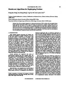
Theorem 4. No fixed order revocable priority algorithm of SSP can achieve approximation ratio better than γ. 1 Proof. Let u1 = 0.2, u2 = 12 γ − 10 ≈ 0.326, u3 = 0.5, and u4 = 0.8. For a data item u, we denote by rank(u) its priority. There are four cases:

1. If rank(u4 ) > rank(u3 ), then the adversarial strategy is shown in Fig. 1.

u3

u4

⊕u3 , ⊖u4 ⊖u3

s1

2 u3

u4

⊕u3 , ⊖u3 ⊘

u3 s2

Fig. 1. Adversarial strategy for rank(u4 ) > rank(u3 ).

If the algorithm terminates via state s1 , then ρ=

u3 kALGk < γ. = kOPTk u4

If the algorithm terminates via state s2 , then ρ=

kALGk u4 = u4 < γ. ≤ kOPTk 2u3

2. If rank(u3 ) > rank(u2 ), then the adversarial strategy is shown in Fig. 2.

2 u2

⊕u2 , ⊖u3 ⊖u2

s1

u3 u2

2 u2

⊕u2 , ⊖u2 ⊘

u3 u2 u2 s2

Fig. 2. Adversarial strategy for rank(u3 ) > rank(u2 ).

If the algorithm terminates via state s1 , then ρ=

kALGk 2u2 = = kOPTk u2 + u3

1 2

γ − 15 + 21 γ −

1 10

=

10γ − 2 < γ. 5γ + 4

If the algorithm terminates via state s2 , then ρ=

kALGk u2 + u3 = ≤ kOPTk 3u2

1 2

1 + 21 γ − 10 5γ + 4 < γ. = 3 3 15γ −3 γ − 2 10

12

2u2

u1

4 u1

⊕u1 , ⊖u2 ⊖3 u1

⊕u1 , ⊖u1 ⊘

2u2

s1 u2

3 u1

u1

⊕u1 , ⊖u2 ⊖2 u1

2 u2

⊕u1 , ⊖u1 ⊘

2u1

u1

2u1

⊕u1 , ⊖u2 ⊖u1

s2

2 u2

⊕u1 , ⊖u1 ⊘

u1 u1

Fig. 3. Adversarial strategy for rank(u2 ) > rank(u1 ).

3. If rank(u2 ) > rank(u1 ), then the adversarial strategy is shown in Fig. 3. If the algorithm terminates via state s1 , then ρ=

2u1 + u2 kALGk = ≤ kOPTk u1 + 2u2

2 5

1 + 21 γ − 10 1 1 = 5 +γ− 5

1 2γ

+ γ

3 10

=

5γ + 3 ≤ γ. 10γ

If the algorithm terminates via state s2 , then ρ=

1 u1 + 2u2 1 kALGk = u1 + 2u2 = + γ − = γ. ≤ kOPTk 5u1 5 5

4. If rank(u1 ) > rank(u2 ) > rank(u3 ) > rank(u4 ), then the adversarial strategy is shown in Fig. 4.

u1 u3

⊕u3 , ⊖u2 ⊖u4

s1

u1 u2 u3 u4

⊕u3 , ⊖u1 ⊘

u2 u3 u4 s2

Fig. 4. Adversarial strategy for rank(u1 ) > rank(u2 ) > rank(u3 ) > rank(u4 ).

If the algorithm terminates via state s1 , then ρ=

u1 + u3 kALGk = = kOPTk u2 + u3

1 5 1 2γ

−

+

1 2

1 10

+

1 2

=

7 < γ. 5γ + 4

If the algorithm terminates via state s2 , then ρ=

kALGk 1 u2 + u3 1 1 = u2 + u3 = γ − ≤ + < γ. kOPTk u1 + u4 2 10 2

As a conclusion, no fixed order revocable priority algorithm of SSP can achieve approximation ratio better than γ. This completes the proof. ⊓ ⊔ Finally, we study adaptive revocable priority algorithms. This is the strongest class of algorithms studied in this paper and arguably represents the ultimate

13

approximation power of greedy algorithms (for packing problems). We show that no such algorithm can achieve an approximation ratio better than δ, and then we develop a relatively subtle algorithm having approximation ratio 0.8 in Theorem 6, thus leaving another gap in what is provably the best approximation ratio possible. Theorem 5. No adaptive revocable priority algorithm of SSP can achieve approximation ratio better than δ. Proof. Let u1 = 13 δ ≈ 0.298 and u2 = 0.5. For a given algorithm, we utilize the following adversary strategy shown in Fig. 5. If the algorithm terminates via

3u1 2u2

⊕u2 ⊖u2

⊕u1 ⊘ u1

2u1 2u2

u1 2 u2

⊕u2 , ⊖u2 ⊘ s1

2u1

u1 u2

u1 u2 ⊕u1 ⊘

3u1

2u1

⊕u2 , ⊖u1 ⊕u1 , ⊖u1 ⊘ ⊖u2

2 u2

s3 u1 u2 u1

⊕u2 , ⊖2u1 ⊖u2 s4 u1 u2

⊕u1 ⊘

⊕u2 ⊖u2

⊕u1 ⊘ 2 u1

3u1

u2

s5

⊕u1 , ⊖u2 ⊖u1

2u1

⊕u2 , ⊖u2 ⊘ s2

3u1

u2

Fig. 5. Adversarial strategy for adaptive revocable priority algorithms.

state s1 or s2 , then ρ=

3u1 kALGk = 3u1 = δ. ≤ kOPTk 2u2

If the algorithm terminates via state s3 or s4 , then ρ=

kALGk u1 + u2 = ≤ kOPTk 3u1

1 3δ

+ δ

1 2

=

2δ + 3 ≤ δ. 6δ

=

4δ < δ. 2δ + 3

If the algorithm terminates via state s5 , then ρ=

2u1 kALGk = = kOPTk u1 + u2

2 3δ 1 3δ

+

1 2

In all three cases, the adversary forces the algorithm to have approximation ratio no better than δ; this completes the proof. ⊓ ⊔

14

We now show an adaptive revocable priority algorithm which achieves approximation ratio 0.8 . The method of developping such an algorithm, or in more general all the algorithms in this paper, is to simutanously study adversaries and algorithms for the same problem; by examining closely the boundary points of a lower bound, it often enhences our understanding of underlying difficulties and in most cases gains us valuable insights as of how to design good algorithms. The example in the lower bound proof suggests that the most “troublesome” items are those near 0.3. This makes sense since if a data item is bigger than 0.4, then we can almost always consider it at a relatively late time since for any solution less than 0.8, we can have at most one such item. Therefore the primary focus is given to data items in the range of (0.2, 0.4). Our algorithm uses an ordering of data items which is determined by its distance to 0.3, i.e., the closer a data item to 0.3, the higher its priority is, breaking tie arbitrarily. Note that this ordering does not make the algorithm fixed order priority, as this ordering may be interrupted if at any point of time a terminal condition is satisfied. The algorithm is described below. Algorithm ADAPTIVE 1: Order data items determined by its distance to 0.3; 2: B := ∅; 3: if the first data item is in (0.2, 0.35) then 4: Bmode := Queue; 5: else 6: Bmode := Queue_1; 7: end if 8: while I contains a data item ∈ (0.2, 0.4] do 9: let u be the next data item in I; 10: I := I ⊖ u; 11: accept u; 12: end while 13: if B contains exactly three data items and all are ∈ (0.2, 0.3] then 14: Bmode := Stack; 15: else 16: Bmode := Optimum; 17: end if 18: while I contains a data item ∈ (0.4, 0.8) do 19: let u be the next data item in I; 20: I := I ⊖ u; 21: accept u; 22: end while Theorem 6. Algorithm

ADAPTIVE

achieves approximation ratio 0.8 for SSP.

It is seemingly a small step from a 0.78 algorithm to a 0.8 algorithm, but the latter algorithm requires a substantially more refined approach and detalied analysis. The merit, we believe, in studying such a class of “simple algorithms”

15

is that the simplicity of the structure suggests algorithmic ideas and allows a careful analysis of such algorithms. Limiting ourselves to simple algorithmic forms and exploiting the flexibility within such forms may very well give us a better understanding of the structure of a given problem and a better chance to derive new algorithms.

5

Conclusion

We analyze different types of priority algorithms for SSP leaving open two approximability gaps, one for fixed order and one for adaptive revocable priority algorithms. It is interesting that such gaps and non-trivial algorithms exist for such a simple class of algorithms and such a basic problem as SSP. We optimistically believe that surprisingly good algorithms can be designed within the revocable priority framework for problems which are currently not well understood. In particular, we believe it is worth considering revocable priority algorithms for the time constrained scheduling problem TCSP and the related job interval scheduling problem JISP (see Bar Noy et al. [5], Chuzhoy et al. [9] and Erlebach and Spieksma [11]).

References 1. Angelopoulos, S. and Borodin, A.: On the power of priority algorithms for facility location and set cover. Algorithmica 40 (2004) 271–291 2. Arrow, K.: Social Choice and Individual Values. Wiley (1951) 3. Aspnes, J., Azar, Y., Fiat, A., Plotkin, S. and Waarts, O.: On-line routing of virtual circuits with applications to load balancing and machine scheduling. Journal of the ACM 44 (1997) 486–504 4. Baptiste, P.: Polynomial time algorithms for minimizing the weighted number of late jobs on a single machine with equal processing times. Journal of Scheduling 2 (1999) 245–252 5. Bar-Noy, A., Guha, S., Naor, J. and Schieber, B.: Approximating throughput in real-time scheduling. SIAM Journal of Computing 31 (2001) 331–352 6. Borodin, A., Nielsen, M., and Rackoff C.: (Incremental) priority algorithms. Algorithmica 37 (2003) 295–326 7. Borodin, A., Boyar, J., and Larsen K.: Priority algorithms for graph optimization problems. Lecture Notes in Computer Science 3351 (2005) 126–139 8. Chrobak, M., Durr, C., Jawor, W., Kowalik, L. and Kurowski, M. A note on scheduling equal-length jobs to maximize throughput. Journal of Scheduling 9 (2006) 71–73 9. Chuzhoy, J., Ostrovsky, R. and Rabani, Y.: Approximation algorithms for the job interval scheduling problem and related scheduling problems. In Proceedings of 42nd Annual IEEE Symposium of Foundations of Computer Science (2001) 348–356 10. Davis, S. and Impagliazzo, R.: Models of greedy algorithms for graph problems. In Proceedings of the 15th Annual ACM-SIAM Symposium on Discrete Algorithms (2004) 381–390 11. Erlebach, T. and Spieksma, F.: Interval selection: Applications, algorithms, and lower bounds. Journal of Algorithms 46 (2003) 27–53

16 12. Fleischer, R. and Wahl, M.: On-line scheduling revisited. Journal of Scheduling 3 (2000) 343–353 13. Garey, M. and Johnson, D.: Computers and Intractability: A Guide to the Theory of NP-completeness. Freeman (1979) 14. Graham, R.: Bounds for certain multiprocessor anomalies. Bell System Technical Journal 45 (1966) 1563–1581 15. Horn, S.: One-pass algorithms with revocable acceptances for job interval selection. Master’s thesis, University of Toronto (2004) 16. Ibarra, O. and Kim, C.: Fast approximation algorithms for the knapsack and sum of subset problem. Journal of the ACM 22 (1975) 463–468 17. Iwama, K. and Taketomi, S.: Removable online knapsack problems. Lecture Notes in Computer Science 2380 (2002) 293–305 18. Kellerer, H., Mansini, R., Pferschy, U. and Speranza, M.: An efficient fully polynomial approximation scheme for the subset-sum problem. Journal of Computer and System Science 66 (2003) 349–370 19. Martello, S. and Toth, P.: Knapsack Problems: Algorithms and Computer Implementations. John Wiley and Sons (1990) 20. Moore, J.: An n-job, one machine sequencing algorithm algorithm for minimizing the number of late jobs. Management Science 15 (1968) 102–109 21. Regev, O.: Priority algorithms for makespan minimization in the subset model. Information Processing Letters 84 (2002) 153–157

17

A

Proof of Theorem 1

Lemma 1. No adaptive irrevocable priority algorithm of SSP can achieve approximation ratio better than α. Proof. We show that for any irrevocable priority algorithm and every small ǫ > 0, ρ < α + ǫ. Let u1 = α ≈ 0.657, u3 = α2 ≈ 0.432,

u2 = 2α3 + α2 ǫ ≈ 0.568, u4 = α2 − α2 ǫ ≈ 0.432;

then for any algorithm, the adversary presents one copy of u1 , u2 , u4 and two copies of u3 to the algorithm. Let u be the data item with highest priority among these four types, then if the algorithm discards u on its first decision, then the adversary can remove the rest of the data items and force infinite approximation ratio. We therefore assume that the algorithm always takes the first data item into its solution, then depending on which is the first data item the algorithm selects, there are four cases: 1. If u = u1 , then the adversary removes two copies of u3 ; since u1 + u2 > 1 and u1 + u4 > 1, the algorithm can take neither of the two, hence kALGk = u1 . On the other hand, u2 + u4 = 1, hence kOPTk = u2 + u4 . Therefore, the approximation ratio is ρ=

α u1 kALGk = = α. = 3 kOPTk u2 + u4 2α + α2

2. If u = u2 , then the adversary removes one copy of u1 and one copy of u4 ; since u2 + u3 > 1, the algorithm can take neither of the two, hence kALGk = u2 . On the other hand, u2 < 2u3 < 1, hence kOPTk = 2u3 . Therefore, the approximation ratio is ρ=

kALGk 2α3 + α2 ǫ ǫ u2 = =α+ . = 2 kOPTk 2u3 2α 2

3. If u = u3 , then the adversary removes one copy of u2 , u3 and u4 ; since u1 + u3 > 1, the algorithm cannot take u1 , hence kALGk = u3 . On the other hand, u3 < u1 < 1, hence kOPTk = u1 . Therefore, the approximation ratio is α2 u3 kALGk = = = α. ρ= kOPTk u1 α 4. If u = u4 , then the adversary removes two copies of u3 ; since u1 + u4 > 1, the algorithm cannot take u1 , hence kALGk = u4 . On the other hand, u4 < u1 < 1, hence kOPTk = u1 . Therefore, the approximation ratio is ρ=

α2 − α2 ǫ kALGk u4 α2 = = < = α. kOPTk u1 α α

18

⊓ ⊔

Therefore, in all cases, ρ < α + ǫ; this completes the proof.

We now give a fixed irrevocable priority algorithm that achieves approximation of α. As justified earlier in Section 3, we only consider relevant data items for the input set; we partition all possible relevant data items into two sets: M and L. A data item u is said to be in class M and L if 1 − α < u ≤ α2 and α2 < u < α respectively; see Fig. 6. We specify the ordering of data items for the fixed

0.343 0.432 1−α

0 S

0.657

2

α M

α L

1 X

Fig. 6. Classification for the fixed irrevocable priority algorithm.

irrevocable priority algorithm: it first orders data items in L non-decreasingly, and then data items in M non-decreasingly. The algorithm, which is described below, uses this ordering to achieve the approximation ratio α.

Algorithm 1 1: 2: 3: 4: 5: 6: 7: 8: 9:

Order data items in L non-decreasingly and then M non-decreasingly; B := ∅; for i := 1 to n do let ui be the next data item in I; I := I ⊖ ui ; if kBk + ui ≤ 1 then B := B ⊕ ui ; end if end for

Lemma 2. There is a fixed order irrevocable priority algorithm, which uses the above ordering, for SSP with approximation ratio α. Proof. It is sufficient to show that Alg. 1 achieves this approximation ratio. Note that if ALG contains more than one data item, the kALGk > 23 > α; hence the algorithm achieves approximation ratio α. Suppose now ALG contains only one data item uj . If uj ∈ M, then |L ∩ I| = 0 and |M ∩ I| = 1. Therefore, we have kOPTk = kALGk = uj ; the algorithm achieves approximation ratio 1. Suppose now uj ∈ L, we then consider data items in OPT. Note that OPT can contain at most two data items; there are five cases:

19

1. If OPT contains exactly one data item ur ∈ M, then |L ∩ I| = 0 and hence uj ∈ M. Since uj ∈ L, this is a contradiction; this case is impossible. 2. If OPT contains exactly one data item ur ∈ L, then the approximation ratio is kALGk α2 uj ρ= > = = α. kOPTk ur α 3. If OPT contains two data items ur , us ∈ M with ur ≤ us , then we have uj + us > 1. Therefore, the approximation ratio is ρ=

1 − us 1 − α2 2α3 kALGk uj > > = = α. = 2 kOPTk ur + us ur + us 2α 2α2

4. If OPT contains two data items ur , us with ur ∈ M and us ∈ L, then ALG should have contained the smallest data item in M ∩ I and the smallest data item in L ∩ I, or the smallest two data items in L ∩ I, and hence a contradiction; this case is impossible. 5. If OPT contains two data items ur , us ∈ L with ur ≤ us , then ALG should have contained the smallest two data items in L ∩ I, and hence a contradiction; this case is impossible. Therefore, Alg. 1 achieves the approximation ratio α.

⊓ ⊔

Theorem 1 is immediate by Lemmas 1 and 2.

B

Proof of Theorem 2

Lemma 3. No non-increasing order revocable priority algorithm of SSP can achieve approximation ratio better than α. Proof. We show that for any non-increasing order revocable priority algorithm and every small ǫ > 0, ρ < α + ǫ. Let u1 = α ≈ 0.657, u3 = α2 ≈ 0.432,

u2 = 2α3 + α2 ǫ ≈ 0.568, u4 = α2 − α2 ǫ ≈ 0.432;

we utilize the following adversarial strategy shown in Fig. 7. If the algorithm terminates via state s1 , then kALGk ≤ u1 . Since u2 + u4 = 2α3 + α2 = 1, we have kOPTk = u2 + u4 . Therefore, the approximation ratio is ρ=

kALGk α u1 = = α. ≤ 3 kOPTk u2 + u4 2α + α2

If the algorithm terminates via state s2 , then kALGk ≤ u2 and kOPTk = 2u3 . Therefore, the approximation ratio is ρ=

kALGk 2α3 + α2 ǫ 1 u2 = = α + ǫ. ≤ 2 kOPTk 2u3 2α 2

20

u1 u2 2 u3 u4 ⊕u1 ⊘ u1

s1 : u1

u2 2u3 u4 ⊕u2 , ⊖u2 ⊖2 u3

u2 ⊕u2 , ⊖u1 ⊖u4 ⊕u3 , ⊖u3 ⊘

u4

s2 : u2

u3

2 u3

⊕u3 , ⊖u2 ⊖u3 s3 : u3

Fig. 7. Adversarial strategy for fixed non-increasing order.

If the algorithm terminates via state s3 , then kALGk = u3 and kOPTk = u1 . Therefore, the approximation ratio is ρ=

kALGk α2 u3 = = = α. kOPTk u1 α

In all three cases, the adversary forces the algorithm to have approximation ratio ρ < α + ǫ; this completes the proof. ⊓ ⊔ We now give a non-increasing order revocable priority algorithm that achieves the approximation ratio α. We use the same partition as shown in Fig. 6; the algorithm is described below.

Algorithm 2 1: 2: 3: 4: 5: 6: 7: 8: 9: 10: 11: 12: 13: 14:

Order data items non-increasingly; B := ∅; Bmode := Queue; for i := 1 to n do let ui be the next data item in I; I := I ⊖ ui ; if kBk + ui ≤ 1 then accept ui ; else if ui ∈ L then accept ui ; else reject ui ; end if end for

21

Lemma 4. There is a non-increasing order revocable priority algorithm of SSP with approximation ratio α. Proof. It is sufficient to show that Alg. 2 achieves this approximation ratio. We prove this by induction on i. At the end of the ith iteration of the for loop, we let ALGi and OPTi be the algorithm’s solution and the optimal solution respectively; these are solutions with respect to the first i data items {u1 , . . . , ui }. We also let ρi to be the current approximation ratio, ρi =

kALGi k . kOPTi k

It is clear that at the end of the first iteration, the algorithm has approximation ratio ρ1 = 1 > α. Suppose there is no early termination and the α-approximation is maintained for the first k − 1 iterations, i.e., kALGi k < α and ρi ≥ α for all i < k; we examine the case for i = k, k ≥ 2. Note that |ALGi | = 1 for all i < k, for otherwise kALGi k ≥ α. The algorithm examines data items in non-increasing order; for data items in L, it always accepts the current one into the solution, no matter whether or not the data item fits; for data items in M, it always rejects the current one if it does not fit. In that sense, it tends to keep the smallest data item in L∩I and the largest data item in M∩I. There are only three possibilities for uk during the k th iteration; it must fall into one of the lines 6, 8 and 10: 1. Line 6: then the algorithm accepts uk into the solution without discarding any accepted data item in the solution. Hence we have |ALGi | = 2, the terminal condition is satisfied. Therefore, the algorithm terminates and achieves approximation ratio α. 2. Line 8: then at the end of (k − 1)th iteration, ALGk−1 contains only uk−1 . Since the terminal condition is not satisfied during the k th iteration, we have uk−1 + uk > 1. Therefore, the algorithm accepts uk into the solution by discarding uk−1 . Note that uk and uk−1 are the two smallest data items examined so far and uk−1 + uk > 1, hence OPTk contains exactly one data item, say ur , in L. Therefore, the approximation ratio is ρk =

α2 uk kALGk k ≥ = = α. kOPTk k ur α

3. Line 10: then uk ∈ M and the algorithm rejects uk , therefore ALGk = th ALGk−1 . Furthermore, at the end of (k − 1) iteration, ALGk−1 contains exactly one data item. Observe that it cannot be a data item in M; for otherwise, the terminal condition is satisfied. Therefore, ALGk−1 contains exactly one data item, say uj , in L. Since the terminal condition is not satisfied during the k th iteration, we have uk + uj > 1; therefore, kALGk k = kALGk−1 k = uj > 1 − uk ≥ 1 − α2 = 2α3 . Note that for all the data items examined so far, uk is the smallest in M, uj is the smallest in L, and uk + uj > 1, hence OPTk can either contain

22

one data item in L or two data items in M; in both cases kOPTk k < 2α2 . Therefore, the approximation ratio is ρk =

2α3 kALGk k = α. > kOPTk k 2α2

We now have shown that in all three cases, the algorithm maintains the approximation ratio ρi ≥ α for i = k; this completes the induction. Therefore, Alg. 2 achieves approximation ratio α. ⊓ ⊔ Theorem 2 is immediate by Lemmas 3 and 4.

C

Proof of Theorem 3

Lemma 5. No non-decreasing order revocable priority algorithm of SSP can achieve approximation ratio better than β. Proof. We show that for any non-decreasing order revocable priority algorithm and every small ǫ > 0, ρ < β + ǫ. Let u1 = 1 − β ≈ 0.220, u2 = 21 β + 41 ǫ ≈ 0.390, u3 = β ≈ 0.780; we utilize the following adversarial strategy shown in Fig. 8.

u1 2u2 u3 ⊕u1 ⊘ u1

2 u2

u3

⊕u2 ⊘

s1 : u1 u2

u1 u2 u2 u3 ⊕u2 , ⊖u2 ⊖u3

⊕u2 , ⊖u1 ⊘ s2 : 2u2

u3

Fig. 8. Adversarial strategy for fixed non-decreasing order.

If the algorithm terminates via state s1 , then kALGk = u1 +u2 and kOPTk = 2u2 . Note that u1 + u2 = 1 − 12 β + 41 ǫ = β 2 + 14 ǫ. Therefore, the approximation ratio is β 2 + 41 ǫ 1 − 21 β + 14 ǫ kALGk u1 + u2 = < β. ρ= = = kOPTk 2u2 β + 12 ǫ β + 21 ǫ

23

If the algorithm terminates via state s2 , then kALGk ≤ 2u2 . Since u1 + u3 = 2 = 1, we have kOPTk = u1 + u3 . Therefore, the approximation ratio is ρ=

kALGk 1 2u2 = β + ǫ. ≤ kOPTk u1 + u3 2

In both cases, the adversary forces the algorithm to have approximation ratio ρ < β + ǫ; this completes the proof. ⊓ ⊔ We now give a non-decreasing order revocable priority algorithm that achieves the approximation ratio β. For all possible relevant data items, we partition them into two sets: M and L. A data item u is said to be in class M and L if 1 − β < u ≤ 21 β and 12 β < u < β respectively; see Fig. 9.

0.220 1−β

0 S

0.390

0.780 β

1 2β

M

L

1 X

Fig. 9. Classification for non-decreasing order.

The algorithm achieves this ratio is surprisingly simple; it basically set Bmode to Stack mode, and accepts each data item in turn; see Alg. 3.

Algorithm 3 1: 2: 3: 4: 5: 6: 7: 8:

Order data items non-decreasingly; B := ∅; Bmode := Stack; for i := 1 to n do let ui be the next data item in I; I := I ⊖ ui ; accept ui ; end for

Lemma 6. There is a non-decreasing order revocable priority algorithm of SSP with approximation ratio β.

24

Proof. It is sufficient to show that Alg. 3 achieves this approximation ratio. We prove this by induction on i. At the end of the ith iteration of the for loop, we let ALGi and OPTi be the algorithm’s solution and the optimal solution respectively; and let ρi be the current approximation ratio. It is clear that at the end of the first iteration, the algorithm has approximation ratio ρ1 = 1 > β. Suppose there is no early termination and the approximation ratio ρi ≥ β is maintained for all i < k, we examine the case for i = k. There are two possibilities. The first case is that kBk+uk ≤ 1, then the algorithm accepts uk into the solution without discarding any accepted data item in the solution. Hence we have kOPTk k ≤ kOPTk−1 k+uk ; for otherwise, we can take OPTk ⊖ uk as OPTk−1 , which leads to a contradiction. Therefore, the approximation ratio is ρk =

kALGk−1 k kALGk−1 k + uk kALGk k ≥ ≥ = ρk−1 ≥ β. kOPTk k kOPTk−1 k + uk kOPTk−1 k

This leaves the case when kBk + uk > 1. Note that the algorithm examines data items in non-decreasing order; u1 is the smallest data item in I and u2 is the second smallest. These two data items are at the bottom of the stack, hence tend to stay in the stack unless we see a data item with sufficient large weight: – Observation 1: if at certain stage of the algorithm, after accepting uk , there is only one data item uk 6= u1 in the stack, then we have u1 + uk > 1; see Fig. 10.

uk−1 .. .

⊕

uk

=

uk

u1

Fig. 10. Stack with one data item.

– Observation 2: if at certain stage of the algorithm, after accepting uk , there are only two data items in the stack and the top of the stack is uk 6= u2 , then we have u1 + u2 + uk > 1; see Fig. 11.

The above two inequalities are useful in our analysis. Now we consider data items in OPTk ; there are six cases:

25

uk−1 .. .

uk

u2 u1

⊕

uk

= u1

Fig. 11. Stack with two data items.

1. If |OPTk | = 1, then OPTk = {uk }. Since the algorithm always accepts the current data item, we have uk ∈ ALGk , and hence ALGk = OPTk . Therefore, the approximation ratio is ρk =

kALGk k = 1. kOPTk k

2. If OPTk contains exactly two data items ur , us ∈ M with ur ≤ us , then we have both u1 and u2 in M ; we now consider data items in ALGk . (a) If |ALGk | = 1, then ALGk = {uk }; by Observation 1, we have u1 + uk > 1. Since ur + us ≤ β, we have 1 − u1 ≥ 1 − 21 β = β 2 . Therefore, the approximation ratio is ρk =

1 − u1 β2 uk kALGk k > ≥ = = β. kOPTk k ur + us ur + us β

(b) If |ALGk | = 2, then

ALGk

= {u1 , uk }; by Observation 2, we have u1 + u2 + uk > 1.

Since ur + us ≤ β, we have 1 − u2 ≥ 1 − 12 β = β 2 . Therefore, the approximation ratio is ρk =

kALGk k 1 − u2 β2 u1 + uk > ≥ = = β. kOPTk k ur + us ur + us β

(c) If |ALGk | ≥ 3, then {u1 , u2 , uk } ∈ ALG. Note that u1 + u2 > 2 − 2β. Therefore, the approximation ratio is ρk =

kALGk k 2 − 2β + us u1 + u2 + uk > 1, > 1 ≥ kOPTk k ur + us 2 β + us

which is a contradiction; this case is impossible. 3. If OPTk contains exactly two data items ur ∈ M and us ∈ L, then we have u1 in M ; we now consider data items in ALGk .

26

(a) If |ALGk | = 1, then

ALGk

= {uk }; by Observation 1, we have u1 + uk > 1.

(3)

Note that u1 + us ≤ ur + us ≤ 1. When the algorithm considers us , u1 is already in the solution. Since the terminal condition is not satisfied, we have u1 + us < β.

(4)

Combining (3) and (4), we have uk > 1 − β + us . Therefore, ρk = (b) If |ALGk | = 2, then ρk =

kALGk k 1 − β + us uk > 1 = > β. kOPTk k ur + us 2 β + us ALGk

= {u1 , uk }. Therefore

kALGk k 1 − β + us u1 + uk > β. > 1 = kOPTk k ur + us 2 β + us

(c) If |ALGk | ≥ 3, then {u1 , u2 , uk } ∈ ALG. Note that u1 + u2 > 2 − 2β. Therefore, the approximation ratio is ρk =

kALGk k 2 − 2β + us u1 + u2 + uk > 1, > 1 ≥ kOPTk k ur + us 2 β + us

which is a contradiction; this case is impossible. 4. If OPTk contains exactly two data items ur , us ∈ L with ur ≤ us , then we have β ≤ ur + ur+1 ≤ ur + us ≤ 1. When the algorithm considers ur+1 , ur is already in the solution; hence the terminal condition is satisfied. 5. If OPTk contains exactly three data items ur , us , ut ∈ M with ur ≤ us ≤ ut , then we have both u1 and u2 in M ; we now consider data items in ALGk . (a) If |ALGk | = 1, then ALGk = {uk }; by Observation 1, we have u1 + uk > 1.

(5)

Note that u1 + ur + us ≤ u1 + us + us+1 ≤ ur + us + ut ≤ 1. When the algorithm considers us+1 , u1 and us are already in the solution. Since the terminal condition is not satisfied, we have u1 + us + us+1 < β. Therefore, u1 + ur + us < β.

(6)

Combining (5) and (6), we have uk > 1 − β + ur + us . Since both ur and us are in M, we have ur + us > 2 − 2β > 21 β. Therefore, ρk =

kALGk k 1 − β + (ur + us ) uk > 1 = > β. kOPTk k ur + us + ut 2 β + (ur + us )

27

(b) If |ALGk | = 2, then

ALGk

= {u1 , uk }; by Observation 2, we have u1 + u2 + uk > 1.

(7)

– If r = 1, then u2 + ur + us ≤ u1 + u2 + us+1 ≤ ur + us + ut ≤ 1. When the algorithm considers us+1 , u1 and u2 are already in the solution. Since the terminal condition is not satisfied, we have u1 +u2 +us+1 < β. Therefore, u2 + ur + us < β.

(8)

– If r > 1, then u2 + ur + us ≤ u2 + us + us+1 ≤ ur + us + ut ≤ 1. When the algorithm considers us+1 , u2 and us are already in the solution. Since the terminal condition is not satisfied, we have u2 +us +us+1 < β. Therefore, the inequality (8) is also satisfied. Therefore, in both cases we have (8). Combining (7) and (8), we have u1 + uk > 1 − β + ur + us . Since both ur and us are in M, we have ur + us > 2 − 2β > 21 β. Therefore, ρk =

kALGk k 1 − β + (ur + us ) u1 + uk > 1 = > β. kOPTk k ur + us + ut 2 β + (ur + us )

(c) If |ALGk | ≥ 3, then {u1 , u2 , uk } ⊆ ALG. Note that u1 + ur + us ≤ u1 + us + us+1 ≤ ur + us + ut ≤ 1. When the algorithm considers us+1 , u1 and us are already in the solution. Since the terminal condition is not satisfied, we have u1 + us + us+1 < β. Therefore, u1 + ur + us < β.

(9)

Then we have ur + us < β − u1 < β − (1 − β) = 2β − 1. Note that u1 + u2 > 2 − 2β. Therefore, ρk =

2 − 2β + ut u1 + u2 + uk kALGk k > > β. ≥ kOPTk k ur + us + ut 2β − 1 + ut

6. If OPTk contains exactly three data items ur , us ∈ M and ut ∈ L with ur ≤ us , then we have 1 β < 2 − 2β + β < u1 + u2 + ut ≤ ur + us + ut ≤ 1. 2 When the algorithm considers ut , u1 and u2 are already in the solution; hence the terminal condition is satisfied. We now have shown that in all six cases, the algorithm maintains the approximation ratio ρi ≥ β for i = k; this completes the induction. Therefore, Alg. 3 achieves approximation ratio β. ⊓ ⊔ Theorem 3 is immediate by Lemmas 5 and 6.

28 Table 2. Corresponding symbols. class (0.2, 0.4] (0.4, 0.8) (0.2, 0.3] (0.3, 0.4] symbol ♦  ▽ △

D

Proof of Theorem 6

For notational convenience, we use the following symbols to denote data items in different classes; see Table 2. The algorithm can be divided into two stages. In the first stage (while loop) data items of type ♦ are processed; in the second stage (while loop) data items of type  are processed. For a given instance, we now assume that the algorithm ADAPTIVE achieves approximation ratio less than 0.8 and try to derive a contradiction. First, we let S = u1 , u2 , . . . , un be the input sequence of data items according to the algorithm’s ordering, and let S1 = u1 , u2 , . . . , um and S2 = um+1 , um+2 , . . . , un be the input sequences of data items for the first stage and second stage respectively. Lemma 7. Let u be the next data item to be examined and B′ = (B ⊕ u). If B′ contains three data items ui , uj , uk , with i < j < k, then (ui , uj , uk ) cannot be any of the following types: (▽, ▽, △), (△, △, ▽),

(▽, △, ▽), (△, ▽, △);

Proof. This is immediate as the total weight of those triples are in [0.8, 1]. Since at each step, the algorithm adaptively checks for a terminal condition, it can detect those triples and terminate early. ⊓ ⊔ Lemma 8. The input sequence S is of one of the following sequence types: 1. 2. 3. 4.

▽, ▽, ▽, . . . , ▽, ▽, ▽; △, ▽, ▽, . . . , ▽, ▽, ▽; △, △, △, . . . , △, △, △; ▽, △, △, . . . , △, △, △;

assuming S1 = u1 , . . . , um and each type has m data items. Proof. This clearly holds if S1 contains at most two data items. Suppose now S1 contains more than two data items; there are four cases: 1. If (u1 , u2 ) = (▽, ▽), then B is in Queue Mode for the first stage. Suppose △ occurs after u2 , then let ui+1 be the first such occurrence; when the algorithm considers ui+1 , {ui−1 , ui } ⊆ B. Since (ui−1 , ui , ui+1 ) = (▽, ▽, △), this contradicts Lemma 7. 2. If (u1 , u2 ) = (▽, △), then B is in Queue Mode for the first stage. Suppose ▽ occurs after u2 , then let ui+1 be the first such occurrence; when the algorithm considers ui+1 , {ui−1 , ui } ⊆ B. Since either (ui−1 , ui , ui+1 ) = (△, △, ▽), or (ui−1 , ui , ui+1 ) = (▽, △, ▽), this contradicts Lemma 7.

29

3. If (u1 , u2 ) = (△, ▽), then we have two cases: (a) If u1 < 0.35, then B is in Queue Mode for the first stage. Suppose △ occurs after u2 , then let ui+1 be the first such occurrence; when the algorithm considers ui+1 , {ui−1 , ui } ⊆ B. Since either (ui−1 , ui , ui+1 ) = (▽, ▽, △), or (ui−1 , ui , ui+1 ) = (△, ▽, △), this contradicts Lemma 7. (b) If u1 ≥ 0.35 then B is in Queue_1 Mode for the first stage. Suppose △ occurs after u2 , then let ui+1 be the first such occurrence; when the algorithm considers ui+1 , {u1 , ui } ⊆ B. Since (u1 , ui , ui+1 ) = (△, ▽, △), this contradicts Lemma 7. 4. If (u1 , u2 ) = (△, △), then we have two cases: (a) If u1 < 0.35, then B is in Queue Mode for the first stage. Suppose ▽ occurs after u2 , then let ui+1 be the first such occurrence; when the algorithm considers ui+1 , {ui−1 , ui } ⊆ B. Since (ui−1 , ui , ui+1 ) = (△, △ , ▽), this contradicts Lemma 7. (b) If u1 ≥ 0.35, then B is in Queue_1 Mode for the first stage. Suppose ▽ occurs after u2 , then let ui+1 be the first such occurrence; when the algorithm considers ui+1 , {u1 , ui } ⊆ B. Since (u1 , ui , ui+1 ) = (△, △, ▽), this contradicts Lemma 7. Therefore, S1 must be of one of the input sequence types above.

⊓ ⊔

Lemma 8 is useful as it eliminates many cases we need to consider. We now give two observations: – Observation I: for the input sequence types 1 and 2, the data items in S1 is non-increasing, and the total weight of the first three data items of S1 is no greater than 1. – Observation II: for the input sequence types 3 and 4, the data items in S1 is non-decreasing. and the total weight of the first three data items of S1 is greater than 0.8. The data items in S2 is non-decreasing in both cases. For convenience, we denote ALG′ the algorithm’s solution at the end of the first stage; we also suppose S is non-empty; for otherwise, the problem becomes trivial. Lemma 9. |OPT| > 1. Proof. Suppose now |OPT| = 1, there are two cases: 1. If S contains a data item of type , then un is the largest data item in S and OPT = {un }. No matter which operational mode B is in, un is always accepted into the solution. Since un is the last data item in S, the algorithm achieves the optimal solution in this case, which is a contradiction. 2. If S does not contain a data item of type , then the entire input sequence S contain exactly one data item of type ♦, hence the algorithm easily achieves the optimal solution, which is a contradiction. Therefore, both cases are impossible, and hence |OPT| > 1.

⊓ ⊔

30

Lemma 10. No feasible solution contains two data items in S2 . Proof. We prove this by contradiction. Suppose there is a feasible solution which contains two data items in S2 , then it is clear that 0.8 ≤ um+1 + um+2 ≤ 1, and um+1 ≤ 0.5; we exam the beginning of the second stage when the algorithm considers um+1 . Note that the algorithm has to reject um+1 , for otherwise, when the algorithm considers the next data item um+2 , the terminal condition is satisfied. 1. If |ALG′ | < 2, then kALG′ k ≤ 0.4. Since kALG′ k + um+1 ≤ 1, the algorithm must then accept um+1 into its solution, which is a contradiction. 2. If |ALG′ | = 2, then B is in Optimum Mode for the second stage. Let ALG′ = {ui , uj }, then we have ui +uj < uj +um+1 < um+1 +um+2 ≤ 1, the algorithm must then accept um+1 into its solution, which is a contradiction. 3. If |ALG′ | = 3, then we have S1 is of either input sequence type 1 or 2; for otherwise, by Lemma 8, either ALG′ = {△, △, △} or ALG′ = {▽, △, △}, and hence kALG′ k > 0.8, which is a contradiction. (a) If ALG′ = {△, ▽, ▽}, then ALG′ = {u1 , um−1 , um }. Since u1 ≥ 0.3, we have 0.4 ≤ um−1 + um ≤ 0.5.

(10)

If there exist a data item in [0.4, 0.5], then combined with (10), that data item will interrupt the ordering and the terminal condition is satisfied. Hence, there exists no data item in [0.4, 0.5], Therefore, No feasible solution contains two data items in S2 . (b) If ALG′ = {▽, ▽, ▽}, then during the second stage, B is in Stack Mode, hence the algorithm must then accept um+1 into its solution, which is a contradiction. Therefore, no feasible solution contains two data items in S2 . This completes the proof. ⊓ ⊔ Lemma 11. |OPT| < 4 ⇒ kOPTk < 0.8. Proof. We prove this by contradiction. Suppose that |OPT| < 4 and kOPTk ≥ 0.8; by Lemma 9, |OPT| > 1. There are two cases: 1. If |OPT| = 2, then let OPT = {ur , us } with ur ≤ us . Note that if (ur , us ) = (, ), then it contradicts Lemma 10. Therefore (ur , us ) = (♦, ), then ur always enters the solution. This is because during the first stage, B is either in Queue_1 Mode or Queue Mode, every data item in S1 gets a chance to enter the solution. Since ur + us ≥ 0.8, us will interrupt the ordering and become the next data item to be examined when ur is in B, hence the terminal condition is satisfied; this is a contradiction. 2. If |OPT| = 3, then let OPT = {ur , us , ut } with ur ≤ us ≤ ut , there are two possibilities:

31

(a) If (ur , us , ut ) = (♦, ♦, ♦), then consider the first three elements in S. If S1 is of either input sequence type 1 or 2, then by Observation I, we have 0.8 ≤ ur + us + ut ≤ u1 + u2 + u3 ≤ 1. Therefore, the terminal condition is satisfied when the algorithm accepts the first, second and third data item; this is a contradiction. If S1 is of either input sequence type 3 or 4, then by Observation II, we have 0.8 ≤ u1 + u2 + u3 ≤ ur + us + ut ≤ 1. Therefore, the terminal condition is satisfied when the algorithm accepts the first, second and third data item; this is a contradiction. (b) If (ur , us , ut ) = (♦, ♦, ), then consider the input sequence S. If S1 is of either input sequence type 1 or 2, then at the end of the first stage, {um−1 , um } ⊆ ALG′ . Since um−1 and um are the two smallest data items, we have 0.8 ≤ um−1 + um + ut ≤ ur + us + ut ≤ 1. Therefore, the terminal condition is satisfied at the end of the first stage; this is a contradiction. If S1 is of either input sequence type 3 or 4, then by Observation II, we have 0.8 ≤ u1 + u2 + u3 ≤ ur + us + ut ≤ 1. Therefore, the terminal condition is satisfied when the algorithm accepts the first, second and third data item; this is a contradiction. Therefore, kOPTk < 0.8. This completes the proof.

⊓ ⊔

Lemma 12. Bmode = Optimum ⇒ kALG′ k < 0.8kOPTk. Proof. Suppose that kALG′ k ≥ 0.8kOPTk, then since B in Optimum Mode during the second stage, kBk is non-decreasing. Therefore kALG′ k ≤ kALGk, the approximation ratio is ρ= which is a contradiction.

kALG′ k kALGk ≥ ≥ 0.8, kOPTk kOPTk ⊓ ⊔

Lemma 13. |ALG′ | = 6 0. Proof. Suppose that |ALG′ | = 0, then S1 is empty. By Lemma 9, |OPT| > 1, hence OPT contains at least two data items in S2 ; this contradicts Lemma 10. Therefore, |ALG′ | = 6 0. ⊓ ⊔ Lemma 14. |ALG′ | = 6 1.

32

Proof. Suppose that |ALG′ | = 1, then S1 contains only one data item. By Lemmas 9 and 10, |OPT| > 1, and OPT contains at most one data item in S2 . Therefore OPT = {u1 , ui }. Since B is in Optimum Mode, then by Lemma 10, the algorithm achieves the optimal solution, which is a contradiction. Therefore, |ALG′ | = 6 1. ⊓ ⊔ Lemma 15. |ALG′ | = 6 2. Proof. Suppose that |ALG′ | = 2, then |OPT| < 4. This is because if |OPT| = 4, S1 is of either input sequence type 1 or 2, and hence |ALG′ | = 3, which is a contradiction. By Lemma 9, |OPT| > 1. There are two cases: 1. If |OPT| = 2, then let OPT = {ur , us } with ur ≤ us . By Lemma 10 and 11, ur is in S1 and kOPTk < 0.8; there are two possibilities: (a) If (ur , us ) = (♦, ♦), then if m = 2, then ur and us are the only two data items in S1 and ALG′ = {ur , us }. Since B is in Optimum Mode during the second stage, the algorithm clearly achieves the optimal solution, which is a contradiction. If m > 2, then S1 is of either input sequence type 3 or 4; for otherwise, |ALG′ | > 2. Therefore ALG′ = {ui , um }, where ui > 0.3; hence we have kALG′ k 0.3 + um 0.7 ui + um > ≥ = > 0.8. kOPTk ur + us 2um 0.8 Since B is in Optimum Mode during the second stage, by Lemma 12, we have kALG′ k < 0.8kOPTk, which is contradiction. (b) If (ur , us ) = (♦, ), then ur must be the largest data item in S1 . This is because kOPTk = ur + us < 0.8. If ur is not the largest data item in S1 , we can always replace it with the largest data item in S1 ; the solution can only increase, and the feasibility is still maintained. If m = 2, then ur ∈ ALG′ . If m > 2, then S belongs to either input sequence 3 or 4; for otherwise, |ALG′ | > 2. Therefore, we also have ur ∈ ALG′ . Since B is in Optimum Mode during the second stage, by Lemma 10, the algorithm achieves the optimal solution, which is also a contradiction. 2. If |OPT| = 3, then let OPT = {ur , us , ut } with ur ≤ us ≤ ut , there are two possibilities: (a) If ALG′ = {▽, ▽} or ALG′ = {▽, △}, then S1 is of input sequence type 1, 2 or 4, and S1 contains only two data items. We then have 0.8 ≤ u1 + u2 + u3 ≤ ur + us + ut ≤ 1. Therefore, the terminal condition is satisfied, which is a contradiction. (b) If ALG′ = {△, △}, then S1 is of either input sequence type 3 or 4, hence |OPT| < 3, which is a contradiction. Therefore, |ALG′ | = 6 2. Lemma 16. |ALG′ | = 6 3.

⊓ ⊔

33

Proof. Suppose that |ALG′ | = 3, then S1 is of either input sequence type 1 or 2; for otherwise, by Lemma 8, either ALG′ = {△, △, △} or ALG′ = {▽, △, △}, and hence kALG′ k > 0.8, the terminal condition is satisfied, which is a contradiction. 1. If ALG′ = {△, ▽, ▽}, then ALG′ = {u1 , um−1 , um }; there are two cases: (a) If |OPT| < 4, then by Lemma 11, we have kOPTk < 0.8. Since we have B in Optimum Mode during the second stage and kALG′ k = u1 + um−1 + um > 0.7, this contradicts Lemma 12. (b) If |OPT| = 4, then if B in Queue Mode during the first stage, then |ALG′ | = 4, which is a contradiction. Therefore, B in Queue_1 Mode during the first stage. If u1 ∈ OPT, then |ALG′ | = 4, which is a contradiction. Therefore, u1 6∈ OPT; by Observation I, kOPTk ≤ u2 + u3 + u4 + u5 . Note that at the same time, we have the following three inequalities: u1 ≥ 0.35, u1 + u2 + u3 < 0.8, u2 + u3

≥ u4 + u5 .

(11) (12) (13)

Combining (11) and (12), we have u2 + u3 < 0.45. Therefore, by (13), kOPTk ≤ u2 + u3 + u4 + u5 ≤ 2(u2 + u3 ) < 0.9. Since we have B in Optimum Mode during the second stage and kALG′ k = u1 + um−1 + um > 0.75, this contradicts Lemma 12. 2. If ALG′ = {▽, ▽, ▽}, then ALG′ = {um−2 , um−1 , um }; there are two cases: (a) If S2 is empty, then there two possibilities. If m = 3, then the algorithm clearly achieves the optimal solution. If m > 3, then kALGk > 0.65. Since um−2 , um−1 and um are the three smallest data items in S, we have |OPT| < 4. By Lemma 11, kOPTk < 0.8. Therefore, the approximation ratio is kALGk 0.65 ρ= > ≥ 0.8, kOPTk 0.8 which is a contradiction. (b) If S2 is non-empty, then since um−2 , um−1 and um are the three smallest data items in S, we have |OPT| < 4. By Lemma 11, kOPTk < 0.8. Since B in Stack Mode during the second stage and um ≤ um−1 ≤ um−2 ≤ 0.3, we then have kALGk > 0.7. Therefore, the approximation ratio is ρ=

kALGk 0.7 > ≥ 0.8, kOPTk 0.8

which is a contradiction. Therefore, |ALG′ | = 6 3. Theorem 6 is immediate by Lemmas 13, 14, 15, and 16.

⊓ ⊔