Combinatorial Algorithms for the Generalized Circulation Problem

Combinatorial Algorithms for the Generalized Circulation Problem∗ Andrew V. Goldberg† Computer Science Department Stanford University Stanford, CA 94305 Serge A. Plotkin‡ Computer Science Department Stanford University Stanford, CA 94305 ´ Tardos§ Eva School of Operations Research & Ind. Eng. Cornell University Ithaca, NY 14853 November 1989 Abstract We consider a generalization of the maximum flow problem in which the amounts of flow entering and leaving an arc are linearly related. More precisely, if x(e) units of flow enter an arc e, x(e)γ(e) units arrive at the other end. For instance, nodes of the graph can correspond to different currencies, with the multipliers being the exchange rates. We require conservation of flow at every node except a given source node. The goal is to maximize the amount of flow excess at the source. This problem is a special case of linear programming, and therefore can be solved in polynomial time. In this paper we present the first polynomial time combinatorial algorithms for this problem. The algorithms are simple and intuitive. Keywords: Combinatorial optimization, network flow, graph algorithms.

∗

Preliminary version of this paper was presented at the 29th Annual IEEE Symp. on Foundations of Computer Science. † Research partially supported by NSF PYI Grant CCR-8858097 and an IBM Faculty Development Award. ‡ The work was done while the author was with Laboratory for Computer Science, M.I.T.,Cambridge, MA 02139, supported by DARPA Contract N00014-87-K-825 and by ONR Contract N00014-86-K-0593. § The work was done while the author was with the Department of Mathematics, M.I.T., Cambridge, MA 02139, partially supported by Air Force contract AFOSR-86–0078.

1

1

Introduction

Consider the following problem in financial analysis. An investor wants to take advantage of the discrepancies in prices of securities at different stock exchanges and of the currency conversion rates. His objective is to maximize his profit by trading at different exchanges and by converting currencies. The generalized circulation problem, considered in this paper, models the above situation, assuming that a bounded amount of money is available to the investor and that bounded amounts of securities can be traded without affecting the prices. The generalized circulation problem is a generalization of the maximum flow problem. Each arc (v, w) in the network has a gain factor γ(v, w) and a capacity u(v, w). If x units of flow enter the arc at v, then x · γ(v, w) units of flow arrive at w. The graph has a special node, called the source. The objective is to find a flow that maximizes the excess at the source. (Alternative formulations of the problem are discussed in Section 2.4.) In the model of the above financial analysis problem, nodes correspond to different currencies and securities, and arcs correspond to possible transactions. Gain factors represent the prices or the exchange rates. For example, an arc with gain factor of 113 from a vertex representing IBM stocks to a vertex representing U.S. dollars models the possibility of selling the stocks at $113 per share. Generalized circulation problem has been studied extensively in the 60’s and early 70‘s [5, 9, 22, 25, 26, 33]. This problem can be used to model many situations which are impossible to express using standard network flows (see e.g., [8, 22]). The gain factors can be used to represent the fact that we loose some fraction of the commodity while transporting it (due to damage, evaporation, theft, etc.) or that the commodity that enters an arc is transformed into a different commodity before leaving it (to model manufacturing processes, currency exchange, etc.). The generalized circulation problem is in many respects similar to the minimum-cost circulation problem, where each arc has a cost per unit of flow in addition to capacity. This relationship, first observed by Onaga [26], has been studied in detail by Truemper [33]. Both problems can be viewed as problems of transporting a commodity from a producer to a consumer. Intuitively, the only difference between the two problems lies in the method of payment for shipping costs: in the case of the minimum-cost circulations, these costs are paid with money; in the case of the generalized circulations – with the commodity itself. The similarity is not only intuitive; the linear programming dual of these problems, as well as optimality conditions, are be expressed in very similar forms. Since the generalized circulation problem is a special case of the linear programming problem (LP), it can be solved in polynomial time using general-purpose LP algorithms, such as the ellipsoid method [20] or Karmarkar’s algorithm [19]. Standard network flow problems (e.g., the maximum flow and the minimum-cost flow problems) are special cases of LP as well, and can be solved in polynomial time using general LP algorithms. They can also be solved by combinatorial algorithms, i.e., algorithms that exploit the combinatorial structure of the underlying network as opposed to being based on analytic ideas like the interior point methods for linear programming. The combinatorial approach to solve standard network flow problems proved to be extremely valuable and lead to algorithms with running times which are far superior to the running time bounds of the algorithms based on the general linear programming techniques. Surprisingly, no polynomial-time combinatorial algorithm for the generalized circulation problem were known. Nevertheless, previous work on combinatorial algorithms for the generalized flow 2

problem produced useful insights into the structure of the problem, which lead to combinatorial algorithms that run in finite time. Special variants of the linear programming simplex method have been developed for the generalized flow problem (see e.g., [5]). These variants give combinatorial methods for solving the generalized network flow problem. Algorithms that iteratively augment the current flow have also been studied (see e.g., [16, 17, 22, 28, 33]). However, no polynomial-time bounds are known for these algorithms.1 This paper develops the machinery which allows us to design polynomial-time combinatorial algorithms for the generalized circulation problem. We present two algorithms, one based on the repeated application of a minimum-cost flow subroutine, and another based on the idea of augmenting along a biggest improvement path [4] and the idea of canceling negative cycles [14, 21]. We assume that the capacities are integers represented in binary, each gain is given as a ratio of two integers, and denote the value of the biggest integer used to represent the gains and capacities by B. Under these assumptions, the first algorithm runs in O(n2 m(m + n log n) log n log B) time and the second in slightly less than O(n2 m2 log n log2 B) time. The fastest general-purpose linear-programming algorithm currently known [34], when applied to the generalized circulation problem, runs in O(m3.5 log(nB)) time. Using techniques of Kapoor and Vaidya [18], this algorithm can be modified to speed up the required matrix inversions by taking advantage of the special structure of the problem; the resulting algorithm runs in O(n2 m1.5 log(nB)) time [34]. Although our time bounds are somewhat worse than the time bound of Vaidya’s specialization of his linear programming algorithm mentioned above, our approach exploits the combinatorial structure of the problem. Therefore we feel that it will lead to bounds that are better than those arising from implementations of general-purpose linear programming methods. A remaining open question is the existence of a strongly polynomial algorithm for the generalized circulation problem. This problem is one of the simplest LP problems for which no strongly polynomial algorithm is known. (See [23, 30, 31, 24] for a discussion of the classes of linear programs known to have strongly polynomial algorithms.) We believe that a combinatorial approach is more likely to lead to a strongly polynomial algorithm for the generalized circulation problem, and view our results as a step in this direction. This paper is organized as follows. Section 2 defines the generalized circulation problem and closely related concepts, and gives their important algorithmic and combinatorial properties. Section 4 introduces the vertex labels, which are used to convert a given instance of the problem into an equivalent instance with several useful combinatorial properties. Section 5 reviews two simple combinatorial algorithms for the generalized circulation problem. Section 6 describes our first polynomial time algorithm, which is based on a minimum-cost flow subroutine. In Section 7 we present our second algorithm, based on the idea of augmenting the flow along a “big improvement” path. The last section contains concluding remarks.

1 Pulat and Elmaghraby [28] claim to have developed a strongly polynomial algorithm based on iterative augmentation of flow. However, the proof in the paper has a major gap, and the method used for the augmenting path selection does not seem to be sophisticated enough to yield a polynomial-time algorithm.

3

2

Definitions and Background

In this section we review the definition of the minimum-cost flow problem, define the generalized circulation problem, and discuss the relationship between them. In particular, we define the notion of Generalized Augmenting Path (GAP) and review the generalization of the flow decomposition theorem for the case of generalized circulations.

2.1

Minimum-Cost Circulation Problem

First we discuss the minimum-cost circulation problem. A circulation network is a directed graph 2 G = (V, E) with arc capacities given by a nonnegative capacity function u : E → R+ ∞ . We assume that G has no multiple arcs, i.e., E ⊂ V × V . If there is an arc from a node v to a node w, this arc is unique by the assumption, and we denote it by (v, w). This assumption is for notational convenience only. We also assume, without loss of generality, that the input graph G is symmetric: (v, w) ∈ E ⇐⇒ (w, v) ∈ E. In the context of the minimum-cost circulation problem we need the following definitions. A pseudoflow is a function f : E → R that satisfies the following constraints: f (v, w) ≤ u(v, w) ∀(v, w) ∈ E (capacity constraints),

(1)

f (v, w) = −f (w, v) ∀(v, w) ∈ E (flow antisymmetry constraints).

(2)

Remark: To gain intuition, it is often useful to think only about the nonnegative components of a pseudoflow (or a generalized pseudoflow, defined in the next section). The antisymmetry constraints reflect the fact that a flow of value x going from v to w can be thought of as a flow of value (−x) from w to v. The negative flow values are introduced only for notational convenience. Note, for example, that one does not need to distinguish between lower and upper capacity bounds: the capacity of the arc (v, w) represents a lower bound on the flow value on the opposite arc. Given a pseudoflow f , the residual capacity function uf : E → R is defined by uf (v, w) = u(v, w) − f (v, w). The residual graph with respect to a pseudoflow f is given by Gf = (V, Ef ), where Ef = {(v, w) ∈ E|uf (v, w) > 0}. An excess Exf (v) at a node v is equal to Exf (v) = −

X

f (v, w).

(3)

(v,w)∈E

We will say that a node v has excess if Exf (v) is positive, and has deficit if it is negative. A circulation is a pseudoflow with zero excess at every node: Exf (v) = 0 (flow conservation constraints). 2

+ R+ ∞ = R

S

{∞}.

4

(4)

A cost function is a real-valued function on arcs c : E → R. Without loss of generality, we assume that costs are antisymmetric: c(v, w) = −c(w, v) ∀(v, w) ∈ E (cost antisymmetry constraints).

(5)

A cost of a circulation f is given by c(f ) =

X

f (v, w)c(v, w).

(v,w)∈E:f (v,w)≥0

The minimum-cost circulation problem is to find a minimum-cost (optimal) circulation in an input network. Next we state two criteria for optimality of a circulation. To state the first criterion, we define the cost of a cycle to be the sum of costs of arcs along the cycle. Theorem 2.1 (Busacker and Saaty [2]) A circulation is optimal if and only if its residual graph contains no negative-cost cycles. To state the second criterion, we need the notions of the price function and the reduced cost function. A price function is a labeling on nodes p : V → R. A reduced cost function with respect to a price function p is defined by cp (v, w) = c(v, w) + p(v) − p(w). These notions, which originate in the theory of linear programming, are crucial for many minimumcost flow algorithms. As linear programming dual variables, node prices have a natural economic interpretation: they can be interpreted as current market prices of the commodity. We can interpret reduced cost cp(v, w) as the cost of buying a unit of commodity at v, transporting it to w, and then selling it. Theorem 2.2 (Ford and Fulkerson [6]) The cost of a circulation f is minimum if and only if there is a price function p such that, for each arc (v, w), cp(v, w) < 0 ⇒ f (v, w) = u(v, w) (complementary slackness constraints).

(6)

Another useful fact about circulations is the decomposition theorem, which states that a circulation can be viewed as a collection of flows along cycles. Theorem 2.3 (Ford and Fulkerson [6]) For every circulation f , there exists a collection of k ≤ m simple cycles C1 , . . . , Ck in G, and k positive numbers, δ1 , . . ., δk , such that an arc (v, w) appears on one of the cycles only if f (v, w) > 0, and for every (v, w) ∈ E f (v, w) =

X

δi −

i:Ci contains (v,w)

5

X

i:Ci contains (w,v)

δi .

2.2

The Generalized Circulation Problem

This section reviews the definitions of generalized pseudoflows, generalized circulations, and the generalized circulation problem. We summarize some combinatorial properties of the generalized pseudoflows and generalized circulations, and describe the correspondence between these properties and the properties of regular circulations and pseudoflows discussed in the previous section. For more detailed discussion of this correspondence, that was first observed by Onaga [26], see Truemper [33]. In the generalized circulation problem, every arc has a gain factor associated with it, with the gains given by a gain function γ : E → R+ \ {0}. We assume (without loss of generality) that the gain function is antisymmetric: γ(v, w) = 1/γ(w, v) ∀(v, w) ∈ E (gain antisymmetry constraints).

(7)

Remark: Recall that the gain factors in our financial analysis problem correspond to currency exchange rates. Though the exchange rates are usually not antisymmetric, it is easy to use multiple arcs to describe them by a network that satisfies gain antisymmetry constraints. In the case of ordinary flows, if f (v, w) units of flow are shipped from v to w, f (v, w) units arrive at w. In the case of generalized flows, if g(v, w) units of flow are shipped from v to w, γ(v, w)g(v, w) units arrive at w. A generalized pseudoflow is a function g : E → R that satisfies the capacity constraints (1) and the generalized antisymmetry constraints: g(v, w) = −γ(w, v)g(w, v) ∀(v, w) ∈ E (generalized antisymmetry constraints).

(8)

If γ(v, w) > 1, then (v, w) is a gain arc; if γ(v, w) < 1, then (v, w) is a loss arc. A gain of a path (cycle) is a product of gains of arcs on the path (cycle). Given a generalized pseudoflow g, the definitions of residual capacities, residual graph, and excesses are the same as for the ordinary pseudoflows. A generalized circulation is a generalized pseudoflow that satisfies conservation constraints (4) at all nodes except at the source node. The input to a generalized circulation problem is a tuple (G = (V, E), u, γ, s), where G is a directed graph, u is a capacity function, γ is a gain function, and s ∈ V is the source. For simplicity we assume that the capacities are finite and nonnegative. As before, for notational convenience, we assume that G is symmetric and has no multiple arcs. Moreover, we assume, without loss of generality, that the residual graph of the zero flow is strongly connected. A value of a generalized pseudoflow g is the excess Exg (s). The output of a generalized circulation algorithm is a generalized circulation of the highest possible value (an optimal generalized circulation). Unless mentioned otherwise, we assume that the capacities are given as integers, each gain is given as a ratio of two integers, and that all integers are represented in binary. We denote the biggest integer used to represent capacities and gains by B. We assume that B ≥ 2. In addition, we denote the maximum product of gain numerators on a simple path or cycle in the input graph by T , and let L denote the least common denominators of the gains of a simple paths and cycles in the network. Clearly, T ≤ B n and L ≤ B 2m . However, T and L are often significantly smaller 6

than implied by the above bounds. In particular, this is the case for some of the problems obtained via reductions. A flow-generating cycle is a cycle whose gain is greater than 1, and a flow-absorbing cycle is a cycle whose gain is less than 1. Observe that if one unit of flow leaves a node v and travels along a flow-generating cycle, more than one unit of flow arrives at v. Thus we can augment the flow along this cycle, that is, we can increase the excess at any node of the cycle while preserving excesses at other nodes by increasing flow along the arcs in the cycle and correspondingly decreasing flow on the opposite arcs, to satisfy the generalized antisymmetry constraints. Recall the financial analysis interpretation of the generalized circulation problem, discussed in the introduction. From the investor’s point of view, a residual flow-generating cycle is an opportunity to make profit. However, it is possible to take advantage of this opportunity only if there is a way to transfer the profit to the investor’s bank account (the source node). This motivates the following definition. A generalized augmenting path (GAP) is a residual flow-generating cycle and a (possibly trivial) residual path from a node on the cycle to the source. Given a generalized circulation and a GAP in the residual graph, we can augment the flow along the GAP, increasing the value of the current circulation. The role of GAPs in the generalized circulation problem is similar to the role of negative-cost cycles in the minimum-cost circulation problem: both can be used to augment the flow and thus improve the value of the current solution. In the case of the maximum-flow problem, the flow is optimal if and only if the corresponding residual graph contains no augmenting paths [6]. A similar result holds for generalized circulations. Theorem 2.4 (Onaga [26]) A generalized circulation is optimal if and only if its residual graph contains no GAPs. Using the linear programming dual of the problem, it is possible to specify an alternate criterion of optimality, similarly to the way it is done for the minimum-cost circulation problem. We refer to the dual variables as prices. As in the context of the minimum-cost circulation problem, a price function p is a labeling of nodes by real numbers. In addition, in the context of the generalized circulation problem, we require p(s) = 1. Node prices can also be interpreted as market prices of the commodity at nodes, which motivates the definition of the reduced cost function. If a unit of flow is purchased at v and shipped to w, then γ(v, w) units arrive at w. Buying the unit at v costs p(v), and selling γ(v, w) units at w returns p(w)γ(v, w). Thus the reduced cost of (v, w) is defined as cp (v, w) = p(v) − p(w)γ(v, w). Linear programming duality theory provides the following optimality criterion, which is similar to the one given by Theorem 2.2 for minimum-cost circulations.

Theorem 2.5 A generalized circulation is optimal if and only if there exists a price function p, such that the complementary slackness conditions (6) hold for each arc (v, w) ∈ E. 7

2.3

Decomposition of Generalized Pseudoflows

Theorem 2.3 states that a circulation can be decomposed into cycles. In this section we show how to decompose a generalized pseudoflow into “elementary” generalized pseudoflows. We start by defining five types of elementary generalized pseudoflows. Given a generalized pseudoflow g, let E(g) denote the set of nodes with excesses and let D(g) denote the set of nodes with deficits. An elementary generalized flow can be of one of the following types, where the type is defined according to the graph induced by the set of arcs on which this elementary generalized flow is positive. Type I A path from D(g) to E(g). It creates a deficit and an excess at the two ends of the path. Type II A flow-generating cycle and a path connecting this cycle to a node in E(g). It creates excess at the end of the path. (If the path ends at the source, this corresponds to a GAP.) Type III A flow-absorbing cycle and a path connecting a node in D(g) to this cycle. It creates deficit at the end of the path. Type IV A cycle with unit gain. It does not create any excesses or deficits. Type V A pair of cycles connected by a path, where one of the cycles generates flow and the other one absorbs it. It does not create any excesses or deficits. Theorem 2.6 (Gondran and Minoux [15]) A generalized pseudoflow g can be decomposed into components g1 , . . . , gk with k ≤ m such that g(v, w) =

X

gi ,

i

where each component gi is an elementary generalized flow that is positive only on arcs (v, w) with g(v, w) > 0, and that belongs to one of the above mentioned types. This decomposition can be found in O(nm) time. Proof : We prove the theorem by induction on the number of arcs with nonzero flow value. Let G′ denote the subgraph of G consisting of the arcs with positive flow value. If G′ is acyclic, then a decomposition consisting only of paths (generalized pseudoflows of Type I) can be found by tracing the flow from some node with deficit to some node with excess. Otherwise, let C be a cycle in G′ . If this cycle has gain 1, then we can subtract flow around the cycle until one arc on the cycle has zero flow value. The subtracted flow is of Type IV, and the theorem follows by induction. Now consider the case when the gain of C is more than 1 (the case when the gain is less than 1 can be treated similarly). Decrease the flow along this cycle until one of the arcs along the cycle has zero flow value, reducing the excess (possibly to a negative value) at one of the nodes v on the cycle, and denote the removed flow by h. Decompose g − h according to the induction hypothesis. If we did not create any deficit, then the decomposition of g − h plus the (Type II) cycle h is a legal decomposition of g. If v has a deficit, this decomposition will include components that create this deficit. These components can be either of Type I or of Type III, and each is responsible for some 8

amount of deficit, such that all the amounts sum up to the deficit at v in g − h. Observe that each one of these components, together with an appropriate fraction of h, corresponds to an element of Type II or Type V in the decomposition of g. To establish the running time, observe that the above procedure decreases the number of arcs with positive flow value in amortized O(n) time.

2.4

Alternative Formulations

The generalized circulation problem can be stated in several ways. In this section we present different formulations of the problem and discuss the relationship among them. Understanding this relationship is important since different practical problems can be modeled in different terms, and certain algorithms seem more natural when applied to certain formulations. Generalized Flow Problem (See [22] under the name of “flows with losses and gains”.) The input to the problem is a graph G = (V, E), a gain function γ : E → R+ \ {0}, a source s, and a sink t. A generalized flow is a function on arcs that satisfies the antisymmetry constraints on all arcs and the conservation constraints on all nodes except s and t. The value of the flow is defined to be the amount of flow into the sink. Among all the generalized pseudoflows of maximum value, the goal is to find a generalized pseudoflow that minimizes the flow out of the source. Generalized Flow with Profit Problem (GFP Problem) The input to this problem is the same as the input to the generalized flow problem plus a number r ∈ R+ that gives the ratio of the price per unit of commodity at the sink to the price per unit of commodity at the source. The goal is to find a generalized flow that maximizes the profit. For a generalized flow g, the profit is rExg (t) + Exg (s). To reduce a generalized flow problem to the GFP problem, chose r to be large enough (but finite); for example, r = B n + 1. The following linear-time reductions show that the GFP problem is equivalent to the generalized circulation problem. Given an instance (G = (V, E), γ, s, t, r) of the GFP problem, we define an equivalent instance of the generalized circulation problem by adding an arc (t, s) with very large (≥ nB 2 ) capacity and a gain of r; and defining s to be the source. Given an instance (G = (V, E), γ, s) of the generalized circulation problem, define an equivalent instance of the GFP problem by adding a new node t to the graph, along with the arcs (s, t) and (t, s), assigning unit gain and very high ( ≥ nB 2 ) capacity to these arcs, and letting r = 1.

3

The Restricted Problem

Instead of solving the generalized circulation problem directly, we will solve a restricted version of the problem. In this section we define the restricted problem and present O(nm)-time reduction of the general problem to the restricted one. Although similar restricted problems were considered before (see, for example, [16, 33]), we were unable to find a similar reduction in the literature. We say that a generalized circulation network is restricted if in the residual graph of the zero 9

flow all flow-generating cycles pass through the source. The restricted problem is a generalized circulation problem on a restricted network. The restricted problem has a simpler combinatorial structure and leads to simpler algorithms. Unless stated otherwise, in the subsequent sections we will refer to the restricted version of the problem under the name of the generalized circulation problem. One of the nice facts about the restricted problem is that the optimality condition given by Theorem 2.4 simplifies in this case, and becomes very similar to Theorem 2.1. Before stating the simplified optimality condition, we prove a lemma that will also be useful later on. Lemma 3.1 Let g be a generalized pseudoflow in a restricted network. 1. If the excess at every node other than the source s is nonnegative, then for every node v there exists a (v, s)-path in the residual graph Gg . 2. If the residual graph of a generalized pseudoflow g has no flow-generating cycles and the excess at every node other than at the source s is nonpositive, then for every node v there exists an (s, v)-path in the residual graph Gg . Proof : The proof is by induction on the number of arcs with positive flow value. Recall that the residual graph of zero flow is strongly connected. Let G′ be the subgraph induced by the arcs with positive flow value. Both statements are easy to prove when G′ is acyclic. Now suppose G′ contains a cycle C. This cycle is in the residual graph of the zero flow and therefore if its gain is more than 1, it has to pass through the source. Consider the case when the gain of C is at most 1. Decreasing the flow along C can only decrease the deficit at some node. The first claim follows by induction. Observe that if there are no flow-generating cycles in the residual graph of g, then the gain of C has to be at least 1, which proves the second claim. The case of C having a gain of more than 1 can be checked in a similar way. Theorem 3.2 (Onaga [25]) Given a restricted problem, generalized circulation g is optimal if and only if the residual graph of g contains no flow-generating cycles. Proof : Clearly, if the residual graph of the generalized pseudoflow has no flow generating cycles, then it has no GAPs, and therefore it is optimal. To see the converse, consider a flow-generating cycle in the residual graph. We have to show that there is a path in the residual graph connecting this cycle to the source. The generalized circulation g has nonnegative excess at every node, and hence, by the the above lemma, there is a path from every node to the source. Corollary 3.3 Given a restricted problem, a generalized circulation g is optimal if and only if the residual graph of g has no negative-cost cycles, with c = − log γ as the cost function. This corollary implies that the optimality of a solution for an instance of the restricted problem can be tested in one shortest path computation. Finally, we show how to reduce the generalized circulation problem to the restricted version of this problem.

10

Theorem 3.4 The generalized circulation problem is O(nm)-time reducible to the restricted problem.

Proof : The reduction works as follows. First, we saturate all gain arcs. More formally, define a generalized pseudoflow h by h(v, w) = u(v, w) h(v, w) = −γ(w, v)u(w, v) h(v, w) = 0

if (v, w) is a gain arc, if (v, w) is a loss arc, otherwise.

For every v ∈ V such that Exh (v) < 0, add an arc (v, s) of gain γ(v, s) = B n + 1 and capacity u(v, s) = −Exh (v). (We also add reverse arcs with capacity 0 to preserve symmetry.) For every v ∈ V such that Exh (v) > 0, add an arc (s, v) of gain γ(s, v) = B n + 1 and capacity u(s, v) = Exh (v)/γ(s, v) (and the reverse arcs with capacity 0 to preserve symmetry). Finally, define h to be ˆ be the extended graph. Then the transformed problem is (G, ˆ uh , γ, s). zero on the new arcs. Let G Intuitively, the new arcs assure that nodes that have positive excess with respect to h are supplied with an adequate amount of “almost free” commodity, and nodes that have deficits with respect to h send adequate amount of commodity to s, whenever possible. Note that the transformed problem is in the restricted form, i.e., all flow-generating cycles pass through the source. Let gˆ be a maximum generalized flow in the transformed problem. Define the generalized pseudoflow g ′ by g ′ (v, w) = gˆ(v, w) + h(v, w) for every (v, w) ∈ E. Observe that the residual graph of g ′ is the restriction of the residual graph of gˆ to arcs in E. A node v ∈ V − s has deficit in g ′ if and only if the arc (v, s) with gain B n + 1 is in the residual graph of gˆ. Similarly, the node v ∈ V − s has excess in g ′ if and only if the arc (s, v) with gain B n + 1 is in the residual graph of gˆ. Decompose g ′ as described in Theorem 2.6. Let X be the set of nodes participating in the elementary generalized flows of Type II in the decomposition, that create excesses at nodes other than the source s. Observe that there are no paths in the residual graph of g ′ from any node in X to the source or to a node with deficit, since such a path will imply a flow-generating cycle in the residual graph of gˆ, which is impossible by Theorem 3.2. Similarly, the decomposition of g ′ can not contain Type I, Type III or a Type V elements, since existence of such elements implies existence of a flow-generating cycle in the residual graph of gˆ. Therefore, g ′ does not have deficits. Subtract the elements of the decomposition that create the excesses at nodes other than s from the generalized pseudoflow g ′ . Let g be the resulting generalized circulation. We claim that g is optimal. Indeed, g does not have either deficits or excesses at nodes other than the source. Moreover, all flow-generating cycles in the residual graph of g pass through some node in X and nodes in X are not connected to the source in the residual graph of g ′ . This implies that there are no GAPs in the residual graph of g. Note that if B is the biggest integer in the input problem, then the biggest integer in the transformed problem can be as high as B n + 1. On the other hand, the transformation can not cause a significant increase in T and L: the corresponding parameters T ′ and L′ of the transformed problem are bounded by B n (B n + 1) ≤ B 2n+1 and B 2m (B n + 1) ≤ B 3m+1 , respectively. 11

4

Vertex Labels and Equivalent Problems

In this section we review the idea of relabeling, which was originally introduced by Glover and Klingman [9] (under the name of scaling). We introduce the notion of canonical relabeling, and give an intuitive explanation of the relationship between the original and relabeled networks. We also prove an “integrality” theorem which will be used to prove termination of our polynomial-time algorithms presented in subsequent sections. Recall the financial analysis interpretation of the generalized circulation problem, described in the introduction, where vertices correspond to different securities or currencies, and arcs correspond to possible transactions. Suppose one country decides to change the unit of currency (for example, Great Britain could decide to introduce the penny as the basic currency unit, instead of the L, or Italy could erase a couple 0’s at the end of its bills). This causes an appropriate update of the exchange rates. Some of the capacities are changed as well (for example, a million L limit on the exchange from L to DM would now read as a limit of 100 million pennies). The operation of changing the units of measure is called relabeling and the equivalent problem obtained by relabeling is called the relabeled problem. Let µ : V 7−→ R+ be a function denoting the number of old units per each new unit at nodes of the network. Given a function µ, we shall refer to µ(v) as the label of v. Definition: Given a function µ : V 7−→ R+ and a network N = (V, E, γ, u), the relabeled network is Nµ = (V, E, γµ, uµ ), where the relabeled capacities and the relabeled gains are defined by uµ (v, w) = u(v, w)/µ(v) γµ (v, w) = γ(v, w)µ(v)/µ(w). Given a generalized pseudoflow g and a labeling µ, the relabeled residual capacity is defined by: ug,µ (v, w) =

u(v, w) − g(v, w) . µ(v)

The following lemma relates pseudoflows in the original and the relabeled networks. Lemma 4.1 If N is a generalized network and g is a generalized pseudoflow in N , then gµ (v, w) = g(v, w)/µ(v) is a generalized pseudoflow in the relabeled network Nµ . Moreover, the residual graphs of g and gµ are the same.

4.1

Canonical Relabeling

Let g be a generalized pseudoflow whose residual graph has the property that all flow-generating cycles go through s (for example, the zero flow in the restricted problem). We shall use two symmetric ways to relabel a residual network. One is the canonical relabeling from the source, and the other is the canonical relabeling to the source. We use the first relabeling when we want to push additional flow from s, and the second when we want to push additional flow into s. The canonical relabeling from the source applies when every node v ∈ V is reachable from the source s via a path in the residual graph of the generalized pseudoflow g. For every node v ∈ V , 12

the canonical label µ(v) is defined to be equal to the gain of the highest-gain simple s-v path in the residual graph. That is, one new unit corresponds to the amount of flow that can reach the node v if one old unit of flow is pushed along the most efficient simple path in the residual graph from s to v, ignoring capacity restrictions along the path. Observe that the highest-gain path is the shortest path when arc lengths are defined to be c(v, w) = − log(γ(v, w)). Because of the assumption that all flow-generating cycles pass through the source, the highest-gain path can be easily found by a single shortest-path computation, since deleting the arcs entering s from the residual graph yields a graph with no negative cycles. The canonical relabeling to the source is defined similarly. It applies if there is a path in the residual graph from every node to the source s. The canonical label µ is defined as the inverse of the gain of the highest-gain simple v-s path in the residual graph. The following important properties of the canonically relabeled problem are easy to prove. (Notice the symmetry between the theorems.) Theorem 4.2 After a canonical relabeling from the source: 1. Every arc e with nonzero residual capacity, other than the arcs entering the node s, has γµ (e) ≤ 1. 2. For every node v, there exists a path from s to v in the residual graph with γµ (e) = 1 for all arcs e on the path. 3. The most efficient flow-generating cycles consist of an (s, v)-path for some v ∈ V with γµ (e) = 1 along the path, and the arc (v, s) ∈ Eg such that γµ (v, s) = max(γµ(e) : e ∈ Eg ). Theorem 4.3 After a canonical relabeling to the source: 1. Every arc e with nonzero residual capacity, other than the arcs leaving the node s, has γµ (e) ≤ 1. 2. For every node v, there exists a path from v to s in the residual graph with γµ (e) = 1 for all arcs e on the path. 3. The most efficient flow-generating cycles consist of an (v, s)-path for some v ∈ V with γµ (e) = 1 along the path, and the arc (s, v) ∈ Eg such that γµ (s, v) = max(γµ(e) : e ∈ Eg ). There is a simple correspondence between the units used for a relabeling and the prices from the linear programming dual of the problem. Intuitively, making the unit at a vertex v smaller, while keeping the price per unit constant, corresponds to increasing the price at v. In other words, changing the unit at v to µ(v) and keeping the price per unit (p(v)) constant has the same effect as keeping the size of the unit and setting the price to p(v) = p(v)/µ(v). If the price at every node is 1, then canonical relabeling from the source corresponds to changing the prices to p(v) = 1/µ(v). Note that, ignoring the arcs entering s, these prices are the marginal costs of the commodity, that is, the minimum prices (per unit) for which one could get some additional amount of the commodity to the nodes. We can reformulate the optimality conditions of Theorem 2.5 to use labels instead of prices. Lemma 4.4 A generalized circulation g in a restricted problem is optimal if and only if there exists a labeling µ such that every arc in the residual graph of the generalized circulation has γµ(e) ≤ 1. 13

We say that a labeling µ is optimal if there exist a generalized circulation g such that g and µ satisfy the conditions of Lemma 4.4. Lemma 4.5 The optimality of a labeling µ for a restricted problem can be checked in one maximumflow computation. Proof : Relabel the network with labels µ. Suppose g is a generalized circulation that satisfies the optimality conditions with µ, and let gµ be the corresponding generalized circulation in the relabeled network. If γµ (v, w) > 1 then, by the optimality conditions, g(v, w) = u(v, w), that is, gµ (v, w) = uµ (v, w). Due to the symmetry, this uniquely defines the flow value on every arc with γµ (e) 6= 1. The labeling µ is optimal if and only if gµ can be extended to a feasible generalized circulation in the relabeled network. Hence, it is sufficient to solve a network flow feasibility problem on the subgraph of the relabeled network induced by the arcs with unit relabeled gain, which can be done via a single maximum flow computation. During a computation one has to keep the size of the numbers under control. The following lemma provides bounds on some of the numbers occurring in the algorithms. Lemma 4.6 Let g be a generalized pseudoflow such that the canonical relabeling from the source (or to the source) in the residual graph applies. Let µ denote the canonical labels. Then T −1 ≤ µ(v) ≤ T and both numerator and denominator of µ(v) are divisors of L, for every v ∈ V . Proof : The label µ(v) is equal to the gain of an s-v path in G, and hence satisfies the above claim, by the definitions of T and L. The following theorem will be used to prove termination for both of our polynomial-time algorithms. For a node v, a generalized pseudoflow g, and labels µ, let Ex g,µ (v) denote the relabeled excess of the node v, that is, the total excess of the pseudoflow corresponding to g in the relabeled network with labels µ (Ex g,µ (v) = Ex g (v)/µ(v)). Consider the subgraph G′ of G induced by the arcs with unit relabeled gain. By Lemma 4.6, in a canonically relabeled network the relabeled capacity of every arc is a multiple of L−1 . The same is true for the residual capacities of all arcs with relabeled gain different from 1. The next theorem states that the latter is almost true for the arcs in G′ . For any subset S, the relabeled residual capacity of arcs of G′ entering S plus the relabeled excesses of the nodes in S is an integer multiple of L−1 . Theorem 4.7 Let g be a generalized pseudoflow whose residual graph contains no flow-generating cycles. Let µ denote the canonical labels when relabeling from the source (or to the source) in the residual graph of a generalized pseudoflow g. For any subset S ⊆ V , X=

X

v∈S

X

Ex g,µ (v) +

ug,µ (w, v)

v∈S;w∈S / and γµ (w,v)=1

is an integer multiple of L−1 . Proof : By Lemma 4.6, the labels, relabeled gain factors, and relabeled capacities, are multiples of L−1 . However, this is not necessarily true for the relabeled residual capacities. First consider an 14

arc with relabeled gain higher than 1. By assumption, the flow on this arc is equal to the capacity, so the flow is a multiple of L−1 . By symmetry, the flow value on an arc (v, w), with relabeled gain of less than 1 is equal to (−γµ(w, v)uµ(w, v)), so it is also a multiple of L−1 . This might not be true for arcs with unit relabeled gain. The main observation is that the value of X is unchanged when the value of the flow is changed on an arc (and its opposite, to preserve the antisymmetry) with a unit relabeled gain. Indeed, if the arc e is contained in S, then changing the flow on e changes the relabeled excess at the two ends of the arc by opposite amounts. On the other hand, if e is outside of S, then it does not affect the expression. Consider an arc e entering S. A change in the flow on e results in the change in the excess at the head of e and in the corresponding change in the residual capacity of e (in the opposite way). Consequently, one can replace the flow value on all arcs with unit relabeled gain by zero without changing the value of the expression. In the resulting generalized pseudoflow all flow values are multiples of L−1 , and therefore every term in the expression is an integer multiple of L−1 .

5

Simple Algorithms

In this section we review two simple algorithms for the generalized circulation problem. The first algorithm is due to Onaga [25] and the second one is due to Truemper [33]. Both algorithms are based on the natural approach of augmenting along flow-generating cycles. Though the algorithms are not efficient, we describe them in order to give some intuition for the polynomial-time algorithms presented in the subsequent sections. The first algorithm, due to Onaga [25], is similar to the minimum-cost flow method of Busacker and Goven [1] and Jewell [17], that augments the flow along a cheapest augmenting path. In the input network, all flow-generating cycles pass through the source. Onaga observed that this property is retained if the augmentation is done along the highest-gain flow-generating cycle. Onaga’s algorithm iteratively augments the generalized circulation along highest-gain flow-generating cycles in the residual graph, until there are no such cycles left. By Theorem 4.2, if all flow-generating cycles pass through the source, then the highest-gain flow-generating cycle can be found by a shortest path computation. Therefore, each iteration of this algorithm consists of a shortest-path computation followed by an augmentation along a flow-generating cycle through the source. By Theorem 3.2, we know that when the algorithm terminates, the resulting generalized circulation is optimal. Like the minimum-cost flow algorithm that augments the flow along the cheapest path, however, this algorithm does not run in finite time [6]. In order to make the running time finite, Truemper [33] uses a maximum flow algorithm as a subroutine to augment flow along all of the highest-gain flow-generating cycles at once, instead of augmenting the flow on a cycle-by-cycle basis. More precisely, consider the residual graph after the canonical relabeling from the source. Let α = max{γµ(v, s) : (v, s) ∈ Eg }, and let Nα be the generalized network with underlying graph Gα that is induced by the arcs with unit relabeled gains and arcs {(v, s) ∈ Eg : γµ (v, s) = α} together with their opposites. Then, by Theorem 4.2, all flow-generating cycles with the highest gain lie in Gα. Observe that any nongeneralized augmentation of flow in Gα , i.e., augmentation that 15

Step 1 Find µ, canonical labeling from the source. If γµ (v, w) ≤ 1 on every arc of the residual graph, then halt (the current circulation is optimal). Otherwise let α = maxe∈Eg γµ (e). Step 2 Let Gα = (V, Eα ) be the network induced by residual arcs with either unit relabeled gain or relabeled gain of α, and their opposites. Find a circulation f ′ in Gα using the residual relabeled capacities, that maximizes. the flow on the arcs with relabeled gain α entering s. Step 3 Update the current solution by setting g(v, w) = g(v, w) + f ′ (v, w)µ(v) ∀(v, w) ∈ E; v 6= s, and set the value g(s, w) ∀w ∈ V to keep the symmetry.

Figure 1: A single iteration of the maximum-flow based algorithm. disregards the gain factors and views Gα as a standard network, corresponds to a valid generalized augmentation in G. Lemma 5.1 An (ordinary) flow in Gα that maximizes the sum of the flow values on the arcs with relabeled gain factor α entering s corresponds to an optimal generalized circulation in Gα. Therefore, by a single maximum-flow computation, we can augment the flow so that there are no flow-generating cycles that pass through the source in Gα , and therefore there are no flow-generating cycles with gain α in the residual graph. The maximum-flow based algorithm proceeds in iterations, where at each iteration we compute the canonical relabeling from the source, construct Gα , compute the appropriate maximum-flow, and interpret the result as an augmentation of the current generalized circulation. See Figure 1 for a more formal description. All flow-generating cycles in the residual graphs of the generalized circulations found throughout the algorithm pass through the source, which guarantees that the canonical relabeling is applicable. The optimality of the solution produced when the algorithm terminates follows from Theorem 3.2. Theorem 5.2 The highest gain of a flow-generating cycle in the residual graph is strictly decreasing from one iteration to another, and therefore the number of iterations is bounded by the number of different gains of simple flow-generating cycles in the original network. Corollary 5.3 If the gain factors in the input are integer powers of 2 (or of any other constant), then the above algorithm runs in polynomial time. Note that the algorithm which is based on path-by-path augmentation may not terminate, whereas the maximum flow-based algorithm terminates in exponential time.

6

Algorithm MCF

In this section we present our first algorithm that solves the restricted version of the generalized circulation problem in polynomial time. Unless stated otherwise, we will refer to the restricted 16

problem as the generalized circulation problem. This algorithm is based on a minimum-cost flow subroutine, and we call it Algorithm MCF. The main idea of the algorithm is best described by contrasting it with the maximum-flow based algorithm presented in the previous section. At each iteration, both algorithms solve a simpler flow problem, and interpret the result as an augmentation in the generalized circulation network. The maximum-flow based algorithm is slow because at each iteration it considers only arcs with unit relabeled gain and some of the arcs adjacent to the source, disregarding the rest of the graph completely. The algorithm presented in this section considers all arcs, assigns cost c(e) = − log γµ to each arc, and solves the resulting minimum-cost circulation problem (disregarding flow gains and losses). The interpretation of a pseudoflow f is a generalized pseudoflow g, such that g(v, w) =

(

f (v, w) if f (v, w) ≥ 0, −γµ (w, v)f (w, v) otherwise.

Note that, as opposed to the case of the maximum-flow based algorithm, where the interpretation of a feasible circulation is a feasible generalized circulation, the interpretation of a minimum-cost circulation leads to a generalized pseudoflow. Whenever the circulation uses arcs with relabeled gain of less than 1, its interpretation has deficits. A connection between a pseudoflow f and its interpretation is given by the following lemma. Lemma 6.1 The residual graphs of a pseudoflow f and its interpretation g as a generalized pseudoflow are the same. The algorithm starts with the zero generalized pseudoflow, which has flow generating cycles in the residual graph. By the definition of the restricted problem, all these cycles pass through the source. Using this fact, we will show that the only iteration that creates positive excesses is the first one, and that the only positive excess created is the one at the source. Each subsequent iteration tries to use this excess to balance deficits at various nodes of the graph, created by interpretation of flow through arcs with relabeled gain of less than 1. In each iteration we find a minimum-cost flow that satisfies the deficits that were left after the previous iteration. Algorithm MCF, shown in Figure 2, maintains a generalized pseudoflow g in the original (nonrelabeled) network, such that the excess at every node other than the source is nonpositive. The algorithm proceeds in iterations. At each iteration it canonically relabels the residual graph, solves the corresponding minimum-cost flow problem in the relabeled network, and interprets the result as a generalized augmentation.

6.1

Analysis of the Inner Loop of the Algorithm

In this section we prove that Algorithm MCF is correct and that an iteration of the algorithm takes polynomial time. The proof that the number of iterations is polynomial is deferred until the next section. The most important property of a minimum-cost flow, for this application, is that its residual graph has no negative cycles. By Lemma 6.1 this yields the following corollary: 17

Step 1 Find µ, canonical labeling from the source. If γµ (v, w) ≤ 1 on every arc of the residual graph and ∀v ∈ (V − s) : Exg,µ (v) = 0, then halt (the current circulation is optimal). Step 2 Introduce costs c(v, w) = − log γµ (v, w) on the arcs of the network. Find a minimum-cost pseudoflow f ′ in the residual relabeled network N with capacities ug,µ that has excess Exf ′ (v) = - Exg,µ (v) for every node v ∈ V − s. Step 3 Let g′ be the interpreted version of f ′ . Update the current solution by setting g(v, w) = g(v, w) + g′ (v, w)µ(v) ∀(v, w) ∈ E.

Figure 2: Inner loop of Algorithm MCF. Corollary 6.2 The residual graphs of the generalized pseudoflows introduced by the algorithm in Step 3 have no flow-generating cycles. Lemma 6.3 The following statements are true for a generalized pseudoflow g that is constructed by Algorithm MCF: 1. The canonical relabeling applies to the residual graph of g. 2. All excesses, except at the source, are nonpositive. Proof : We will prove the lemma by induction on the number of iterations. The second statement is clearly true before the first iteration. To prove the first statement, recall the assumption that the residual graph of the zero generalized pseudoflow is strongly connected. Also, by the definition of the restricted problem, all flow-generating cycles in the residual graph of the zero generalized pseudoflow pass through the source. Therefore we can apply canonical relabeling from the source. Now consider a generalized pseudoflow g constructed by an iteration. Assume that the generalized pseudoflow before the iteration satisfies the statements of the lemma. By Corollary 6.2, the residual graph of g has no flow-generating cycles, and therefore, by Lemma 3.1, every node is reachable from the source in the residual graph of g. Hence, we can compute the canonical relabeling from the source at Step 1, which proves the first statement of the lemma. Moreover, the absence of flow-generating cycles in the residual graph of the generalized pseudoflow in the previous iteration implies that there are no arcs with relabeled gain of more than 1 after Step 1 of this iteration. Therefore, the interpretation of flow f ′ , computed at Step 2, can create only deficits, which proves the second statement for all iterations except the first. The residual graph of the zero generalized pseudoflow g before the first iteration can contain flow-generating cycles. However, all of these cycles pass through the source. Moreover, after the relabeling, all arcs with relabeled gain of more than 1 enter the source. Therefore, the only node that can have a positive excess after the interpretation of the flow f ′ is the source. Lemma 6.4 For a generalized pseudoflow g and the labeling µ after Step 1, there exists a pseudoflow f ′ in the relabeled residual network of g with Ex f ′ (v) = −Ex g,µ (v) for every node v ∈ V − s. Proof : Let g be a generalized pseudoflow at the beginning of an iteration. Decompose it according to Theorem 2.6. The types of elementary pseudoflows that can contribute to deficits are paths 18

from nodes with deficits to the source and paths from nodes with deficits to flow-absorbing cycles. Existence of a flow-absorbing cycle in the decomposition implies that there are flow-generating cycles in the residual graph of g, which contradicts Corollary 6.2, and therefore there are no flowabsorbing cycles in the decomposition. Consider a subset of the nodes S containing the source. By the previous lemma, the only node that can have an excess is the source. Therefore what we have to prove is, that the sum of the relabeled residual capacities of the arcs entering S is no less than the sum of the relabeled deficits of nodes not in S. Consider a (v, s)-path in the decomposition where v 6∈ S, and let (w1, w2 ) be an arc on this path that enters S. Recall that one of the properties of the decomposition is that (w2 , w1) is an arc of the residual graph and arc (w2 , w1) is not used by any elementary pseudoflow in the decomposition. By Corollary 6.2, there are no flow-generating cycles in the residual graph of g, and hence the relabeled gain of every arc in the residual graph of g is at most 1. Therefore, the sum of deficits created by the paths in the decomposition that use this arc is at most the relabeled residual capacity of the opposite arc (w2 , w1). The above lemmas show that the algorithm can proceed until a generalized circulation is found. By Corollary 6.2 and Theorem 3.2, the generalized circulation found is optimal. Hence, we have proved the following theorem. Theorem 6.5 Each iteration of the algorithm can be implemented in polynomial time, and the generalized circulation g, produced by the algorithm upon termination, is optimal.

6.2

Bounding the Number of Iterations

Consider a generalized pseudoflow g at the beginning of an iteration. The fact that there are deficits and that there are no flow-generating cycles in the residual graph means that the current excess at the source is an overestimate on the value of the maximum possible excess. It is easy to see that the sum of the deficits (after the relabeling) at all the nodes except at the source is a lower bound on P the amount of the overestimation. This suggests to use this value, Def(g, µ) = v6=s (−Ex g,µ (v)), as a measure of the proximity of a generalized pseudoflow to an optimal generalized circulation. First we show that if Def (g, µ) is very small, then the algorithm terminates after one more iteration. Theorem 6.6 If Def (g, µ) < L−1 before Step 2 of an iteration, then the algorithm produces an optimal generalized circulation at the end of Step 3 of this iteration. Proof : We claim that the pseudoflow f ′ , computed at Step 2 of this iteration, uses zero cost arcs only. To see this, consider a set of nodes S containing the source s. We have to argue that the sum of the relabeled deficits of the nodes not in S is at most equal to the sum of the relabeled residual capacities of the zero cost arcs leaving S. Clearly, the difference is at most Def (g, µ) < L−1 . Applying Theorem 4.7 to the complement of S shows that this difference is an integer multiple of L−1 . Therefore, it is nonpositive. 19

The interpretation g ′ of a pseudoflow f ′ that uses zero cost arcs only is equal to the pseudoflow. Therefore, no deficits are left after Step 3. The lemma follows because the residual graph contains no flow-generating cycles throughout the algorithm (by Corollary 6.2). An important observation is that the labels µ are monotonically decreasing during the algorithm. The next lemma relates the decrease in the labels to the price function from the minimum-cost flow computation. Let p′ denote the optimal price function associated with the pseudoflow f ′ found in Step 2. Assume, without loss of generality, that p′ (s) = 0. Lemma 6.7 Let f ′ be the minimum-cost pseudoflow found in Step 2 of an iteration, and let p′ be the associated price function. For each node v, the canonical relabeling in Step 1 of the next iteration ′ decreases the label µ(v) by at least a factor of 2p (v) . Proof : The decrease in the label of a node v is computed by finding a shortest path in the residual graph from s to v. The price function p′ is optimal, and hence the reduced costs of the arcs in the residual graph are nonnegative. Therefore, the length of any (s, v) path is at least p′ (v) − p′ (s). For the analysis of the algorithm we decompose the minimum-cost flow into paths, and consider the paths one-by-one. The decomposition is based on the following lemma. Lemma 6.8 (Ford and Fulkerson [6]) Let f be a minimum-cost flow that satisfies given (nonnegative) demands at every node other than s and let p be an optimal price function such that p(s) = 0. The flow f can be decomposed into cycles and paths from s to the other nodes in such a way that the cycles and the paths are in the residual graph of the zero flow, the cycles have nonpositive cost, and the cost of the paths ending at a node v is at most p(v). Proof : For every node v ∈ V add the arcs (v, s) and (s, v). Extend the flow f to these arcs, so that it becomes a circulation. Define the cost of an arc (v, s) by c(v, s) = −p(v). The new arcs have zero reduced cost, and hence the circulation is of minimum cost. The lemma is proved by applying Theorem 2.3 to decompose this circulation into cycles. Note that the arcs opposite to the ones that belong to the cycles of the theorem are in the residual graph of the circulation. Therefore, the cycles have nonpositive cost. Any cycle that uses a new arc (v, s) corresponds to (s, v)-paths in the original graph. The key idea of the analysis is to distinguish two cases: Case 1, where the flow f ′ can be decomposed into “cheap” paths, (e.g., p′ (v) is small, say p′ (v) < log 1.5, for every v ∈ V ); and Case 2, where there exists v ∈ V such that p′ (v) is “large” (≥ log 1.5). We show that in the first case Def (f, µ) decreases significantly, while in the second case, by Lemma 6.7, some of the labels decrease significantly. Using Theorem 6.6 and Lemma 4.6, we prove that neither case can occur too many times. The following lemma is used to estimate the total deficit created when interpreting a flow as a generalized pseudoflow.

20

Lemma 6.9 Let f ′ be a flow along a simple path P from s to some other node v that satisfies one unit of deficit at v. Let g ′ be the interpretation of f ′ as a generalized pseudoflow. Assume that all relabeled gains along the path P are at most one, and denote them by γ1 , . . ., γk . Then after augmenting by g ′ , Q the unit of deficit at v is replaced by deficits that sum up to at most ( 1≤i≤k γi)−1 − 1.

Proof : The deficit created at the ith node of the path is (1 − γi ), for i = 1, . . . , k. Using the assumption that the gain factors along the path are at most 1, the sum of the deficits can be bounded by k X i=1

(1 − γi) ≤

k X 1 − γi 1 = Qk Qi i=1

j=1

γj

i=1

γi

− 1.

(9)

Using this lemma and Theorem 2.6, we bound the value of Def (g, µ) after an application of Step 3. Let p′ be an optimal price function associated with the flow f ′ , such that p′ (s) = 0. Let β = maxv∈V p′ (v) denote the maximum price. Lemma 6.10 The value of Def (g, µ) after an application of Step 3 can be bounded by 2β − 1 times its value before the Step. Proof : Use Lemma 6.8 to decompose f ′ into paths and cycles. Interpret the pseudoflow f ′ by interpreting the cycles and the paths one-by-one. The costs associated with the arcs of the residual graph of the generalized pseudoflow g are nonnegative, and therefore the cycles in the decomposition consist of zero-cost arcs only. Interpretation of the flow along these cycles does not change the value of the flow on any arc; in particular it does not create deficits. By Lemma 6.9, when interpreting a ′ path from s to v, the deficit at v is replaced by deficits that sum up to at most 2p (v) − 1 ≤ 2β − 1 times the deficit at v satisfied by this path. Corollary 6.11 If p′ (v) < log 1.5 for every node v, then Def (g, µ) decreases by a factor of 2 during the application of Step 3. The remaining difficulty is the fact that the function Def (g, µ) can increase, either when the canonical relabeling is done in Step 1 or in Step 3 when Case 2 applies. If Def (g, µ) has increased by some factor during relabeling (Step 1), or after interpretation of f ′ (Step 3), however, then at least one of the nodes is relabeled by the same factor, as it is shown by the following lemma. Lemma 6.12 If either during Step 3 of one iteration or Step 1 of the next one, Def (g, µ) increases by a factor of α, then the label of some node decreases by at least a factor of α during Step 1 of the second iteration. Proof : The increase in Def (g, µ) during Step 1 is due to relabeling, and hence the deficit at a node can increase during this Step by a factor of α if and only if the label at this node decreases by the same factor. By Lemma 6.10, the increase in Def (g, µ) during Step 3 is bounded by 2β , where 21

β = max p′ (v). Hence, if Def (g, µ) increases by α during this step, there exists a node v such that p′ (v) ≥ log α. By Lemma 6.7, this means that µ(v) decreases by at least α during Step 1 of the next iteration. Combining the above results, we can bound the overall growth of Def (g, µ) during an execution of the algorithm (i.e., the product of all of the factors by which Def (g, µ) increases during the algorithm). Lemma 6.13 The growth of the function Def (g, µ) throughout an execution of the algorithm is bounded by a factor of T O(n). Proof : The function Def (g, µ) can increase either as a result of Step 1 or Step 3. By the above lemma, such increase is followed by a decrease in the label of one of the nodes by at least the same factor during the subsequent relabeling. The claim follows from Lemma 4.6, that limits the decrease of the label of any node. Lemma 4.6 implies that Case 2 cannot occur too many times. The above lemma helps to bound the number of times Case 1 can occur. Theorem 6.14 The algorithm terminates in O(n log T ) = O(n2 log B) iterations. Proof : Lemmas 4.6 and 6.7 show that Case 2 cannot occur more than O(n log T ) times. When Case 1 applies, the value of Def (g, µ) decreases by a factor of 2. The value of Def (g, µ) is at most O(nBT ) after the first iteration, and by Theorem 6.6, the algorithm terminates when this value decreases below L−1 . Lemma 6.13 limits its increase during the algorithm. Hence, Case 1 cannot occur more than O(n log T ) times. To get a bound on the running time, we must decide which minimum-cost flow algorithm to use as a subroutine. The best choice turns out to be Orlin’s strongly polynomial algorithm [27]. Theorem 6.15 The above generalized circulation algorithm can be implemented so that it will use at most O(n2 m(m + n log n) log n log B) arithmetic operations on numbers whose size is bounded by O(m log B). Remark: The choice of a strongly polynomial minimum-cost flow algorithm is somewhat surprising, since our algorithm is not strongly polynomial. The reason for this choice is that the current best scaling algorithms would give worse running times, even when the size of the numbers in the input is small. Observe that the number of bits needed to represent the capacities of the intermediate minimum-cost flow problems can be as high as m log B, which would make any known capacityscaling algorithm too slow. The classical cost-scaling algorithms cannot be used directly because the costs are (irrational) logarithms of rational numbers. A cost-scaling algorithm can be constructed based on the idea of ǫ-optimality, as done in [10, 12]. Note that the gain of a flow-generating cycle n can be as small as 2−O(B ) , and hence the absolute value of the cost of a negative cycle can be as small as B −O(n) . Consequently, the required precision seems to be Ω(B −n ), and therefore the known cost-scaling algorithms are too slow as well. 22

7

The Fat-Paths Algorithm

Recall that a GAP is defined to be a flow-generating cycle with an augmenting path connecting this cycle to the source. A natural way to make progress towards an optimal solution is to increase the flow along a GAP. We call this a generalized augmentation. Clearly, if the augmentations are done along arbitrary GAPs, we do not get a polynomial-time algorithm. One way to improve the running time is to execute only those generalized augmentations that result in a significant progress towards an optimal solution. We divide a generalized augmentation into two parts: augmenting the flow along a flowgenerating cycle and bringing the created excess to the source. Our algorithm first saturates all flow-generating cycles, creating excesses at various nodes of the graph, and only then looks for augmenting paths from nodes with excess to the source. This method does not create deficits. A natural way to measure the progress of this algorithm is by the difference between the excess at the source in the current generalized pseudoflow and the excess at the source in the optimal solution. This difference is called the excess discrepancy. We shall show that if the excess discrepancy is very small, a single maximum-flow computation produces an optimal solution (similarly to Theorem 6.6). Consider an augmenting path with an excess in the beginning of the path. Even if this excess is very large, the increase in the excess at the source caused by an augmentation along this path is limited, and depends on both the capacities and the gains of arcs on the path. We call this limit the fatness of the path. A simple v-s path is ∆-fat if, given unlimited supply at v, at least ∆ units of flow can be sent to s along this path. An arc is ∆-fat if it belongs to a ∆-fat path. Saturating all the flow-generating cycles before bringing the excesses to the source facilitates the search for ∆-fat paths. The section consists of three parts. In the first part we describe the Fat-Path algorithm, assuming existence of the Fat-Augmentation and the Cancel-Cycles procedures, and discuss the correctness and the running time of the algorithm. The second part presents the Fat-Augmentation procedure. This procedure finds a ∆-fat path in the residual graph and augments the flow along it. The third part of this section is devoted to the description of the Cancel-Cycles procedure, which transforms a generalized pseudoflow with flow-generating cycles in its residual graph into a generalized pseudoflow with no such cycles, without creating any deficits.

7.1

Fat-Path Algorithm - Overview

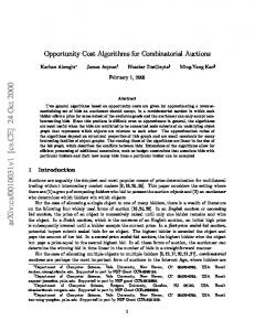
The Fat-Path algorithm, described in Figure 3, solves the restricted problem in phases. The goal of each phase is to decrease the bound on the excess discrepancy by at least a constant factor. The input and output of a phase is a generalized pseudoflow with nonnegative excesses. Each phase consists of three stages. The input to the first stage is a generalized pseudoflow with nonnegative excesses and, possibly, with flow-generating cycles in the residual graph. This stage uses procedure Cancel-Cycles, described in Section 7.3, to cancel all such cycles, creating new excesses at various nodes of the graph. In the second stage we test whether it is possible to bring all the excesses to the source over the most efficient residual paths. This test is performed by canonically relabeling to the source and 23

Stage 1 Cancel all flow-generating cycles by calling the Cancel-Cycles procedure. Stage 2 Compute µ, the canonical labeling to the source. Let E ′ be the set of all arcs with unit relabeled gain. Consider nodes with excess as sources with capacity bounded by the value of their relabeled excess, and compute maximum flow f ′ from these nodes to the source in the graph induced by the arcs in E ′ with the relabeled residual capacities. Update the generalized pseudoflow g by setting g(v, w) = g(v, w) + f ′ (v, w)µ(v) ∀(v, w) ∈ E ′ . Terminate if ∀v ∈ V − s : Ex g (v) = 0. Stage 3 Repetitively call Fat-Augmentation procedure to augment the flow along ∆-fat paths from nodes with excess to the source, as long as such paths exist. Set ∆ = ∆/2.

Figure 3: A single phase of the Fat-Path algorithm. then computing a maximum flow in the graph induced by the unit relabeled gain arcs. Observe that by Lemma 3.1, the canonical relabeling to the source applies. There are no flow-generating cycles in the residual graph after the first stage, and an augmentation of the flow along arcs with a unit relabeled gain does not create such cycles. Therefore, if we succeed in bringing all excess to the source using these arcs, the resulting generalized circulation is optimal, and the algorithm terminates. This stage may be viewed as a variation of a single iteration of the maximum-flow based algorithm, described in Section 5. The input to the third stage is a generalized pseudoflow with nonnegative excesses and no flow-generating cycles, and a “fatness” parameter ∆ (initially set to B 2 ). This stage iteratively augments the flow on ∆-fat paths from nodes with excess to the source, reducing the excess at the starting node of the path and increasing the excess at the source. The stage continues until there are no more ∆-fat paths from nodes with excess to the source. We shall show that throughout this stage there are no flow-generating cycles in the graph induced by ∆-fat arcs. Before the next phase, the value of ∆ is divided by 2. The following lemma indicates that the excess discrepancy is a good measure of progress. Lemma 7.1 If the excess discrepancy is below L−1 , and there are no negative excesses and no flowgenerating cycles in the residual graph, then all the excesses are brought to the source by Stage 2 of the Fat-Path algorithm. Proof : We claim that after Stage 2 the excess discrepancy at the source is an integer multiple of L−1 . This means that the excess discrepancy decreases by at least L−1 in between any two iterations, which directly implies the lemma. Consider the generalized pseudoflow g before Stage 2. Let (S, S) be the cut saturated by the maximum flow computation in Stage 2, such that there are no excesses left in S and s ∈ S. Let µ denote the canonical labels computed during this stage. After this stage, the excess at the source is equal to the sum of Ex g,µ (v) for v ∈ S plus the sum of the relabeled residual capacities of the arcs with relabeled gain 1 entering S, i.e. all the excesses in S are brought to the source. Applying Theorem 4.7 to V ′ = S, the pseudoflow g, and the labels µ, we conclude that this sum is an integer multiple of L−1 . 24

The following lemma bounds the excess discrepancy in terms of ∆. Lemma 7.2 The excess discrepancy at the end of a phase is at most O(m∆). Proof : Let g be a generalized pseudoflow at the end of a phase and let g ∗ be an optimal generalized circulation. Let E + = {e|g ∗(e) > g(e)} be the arcs with positive residual flow, and let G+ = (V, E +). The residual pseudoflow g ∗ − g can be decomposed according to Theorem 2.6. The arcs opposite to the ones used by the cycles in the decomposition are in the residual graph of the generalized circulation g ∗ , and therefore the decomposition consists only of paths from nodes with excess to the source, GAPs, and unit-gain cycles. Note that each one of these paths, GAPs, and cycles is in G+ . There are at most O(m) paths and GAPs used, and therefore it is sufficient to show that each one of them contributes at most ∆ to the excess at the source. First, consider paths from excesses to the source. By construction, no path in Gg from excess to the source is ∆-fat. Also, we have E + ⊆ Eg . Hence, there are no ∆-fat paths in G+ either. Therefore, a path cannot contribute more than ∆ to the excess at the source. By Lemma 7.8, the subgraph of Gg induced by the ∆-fat arcs has no flow-generating cycles. We know that E + ⊆ Eg , and therefore every flow-generating cycle in G+ has at least one arc that is not ∆-fat. Consider a GAP in the decomposition and let (v, w) be a non-∆-fat arc along the flow-generating cycle in the GAP. The contribution of this GAP to the excess of the source is bounded by the fatness of the (v, s)-path in the GAP. The arc (v, w) is not ∆-fat, which implies that the fatness of this path is less than ∆. In Sections 7.2 and 7.3, we prove that the Fat-Augmentation and the Cancel-Cycles procedures can be implemented to run in O(m + n log n) and O(mn2 log n log B) time, respectively. Thus, we have the following theorem: Theorem 7.3 The Fat-Path algorithm runs in O(m2 n2 log n log2 B) time. Proof : By Lemmas 7.1 and 7.2, the algorithm terminates after O(m log B) phases. An augmentation either decreases the number of nodes with excess or decreases the excess discrepancy by at least ∆. By Lemma 7.2, this gives an n + 2m bound on the number of augmentations per phase. Remark: Bruce Maggs [personal communication] has observed that the work in the first and third stages is not well balanced, and one can slightly improve the running time by better balancing. Consider the variant of the algorithm where the parameter ∆ is decreased by a factor α (instead of 2) after every stage. In this variant the number of augmentations in the third stage is at most n + αm per phase. The work required for the other two stages is unchanged. The number of phases log n is logα L (instead of log L). The best choice of α is n2m+n . The resulting running time is log n log B 2

log n log B O(m2 n2 log(n2 /m)+log log n+log log B ), which is somewhat better than the one in Theorem 7.3.

7.2

Fat-Augmentation

The procedure Fat-Augmentation is the core of the Fat-Path algorithm. It finds a node with excess such that the source is reachable from this node through a ∆-fat path, then finds the highest-gain 25

Initialize: Start with an empty tree. For all v ∈ V − s, set Gain(v) = 0. Set Gain(s) = 1 and Father(s) = s. Step 1 while there are nodes outside the tree with nonzero Gain do a) Let v be a node not in the tree with the maximum Gain. b) Add the arc (v, Father(v)) to the tree. c)For every neighbor w of v (i.e., (w, v) ∈ E), if ug,µ (w, v)γµ (w, v)Gain(v) ≥ ∆ and Gain(w) < Gain(v)γµ (w, v), then update Gain(w) = Gain(v)γµ (w, v) and Father(w) = v. Step 2 Relabel the nodes in the tree using µ(v)Gain(v) as the new label of node v (so that the relabeled gain of the tree arcs becomes 1). Step 3 If there exists a node with excess in the tree, augment the current generalized pseudoflow from this node to s along the unique path in the tree.

Figure 4: The Fat-Augmentation algorithm.

∆-fat augmenting path from this node to the source, and augments. First we describe a simple (but not the most efficient) version of the algorithm. Consider a highest-gain augmenting path from a node r to the source. Either this path is ∆-fat, or the capacity of the arc (v, w) that would be saturated when the flow is augmented along this path, times the gain of the part of the path from v to the source, is below ∆. In this case we call (v, w) critical. The observation that a critical arc cannot be ∆-fat leads to a simple algorithm. First, find a highest-gain path from a node with excess, and check its fatness. If it is ∆-fat, we are done. If not, look for a critical arc, delete this arc from the set of arcs considered when searching for a highest-gain path, and repeat. It is important to note that if an augmentation is done along the highest-gain ∆-fat path, then disregarded arcs do not become ∆-fat. The above algorithm runs in polynomial time, but its running time can be improved. A faster method, proposed to us by Bob Tarjan [personal communication], is the one described in Figure 4. The main idea is to recognize and disregard arcs that are not ∆-fat while constructing a highestgain path. Let G∆ g denote the graph induced by the ∆-fat arcs in the residual graph of g. We search for a tree in G∆ g that is rooted at s, such that the path in this tree from any node to the source s has the highest gain among all ∆-fat paths from this node to the source. We call a tree with this property the “Max-Gain” tree. In order to improve the efficiency of finding this tree, we maintain a set of labels µ, such that all ∆-fat arcs have relabeled gains of at most 1. In particular, these labels guarantee that there are no flow-generating cycles in G∆ g . The input to Fat-Augmentation is a parameter ∆, generalized pseudoflow g, and a set of labels µ, such that the relabeled gain γµ of arcs in G∆ g is at most 1. The output is a generalized pseudoflow g ′ , together with updated labels µ′ , such that the relabeled gain of the arcs in G∆ g ′ with respect to ′ µ is at most 1. The procedure can be viewed as a search for a shortest-path tree in G∆ g , where the length of an arc with relabeled gain γµ is − log γµ . There are no ∆-fat arcs with relabeled gain of above 1, and therefore the ∆-fat tree can be “grown” as in the Dijkstra’s shortest-path algorithm. 26

Initially, the ∆-fat tree consists only of s. With each node v, we associate Gain(v), which is the maximum gain of a ∆-fat path found so far from v to s. We initialize Gain(v) = 0, for all v ∈ V − {s}. Like in the Dijkstra’s shortest path algorithm, at each iteration we find a node v that has the largest Gain among the nodes not in the tree, and add it to the tree. The difference is in the way we update the Gain of its neighbors. An arc (v, w) is disregarded by the algorithm if ug,µ (v, w)Gain(w)γµ(v, w) < ∆. We show below that an arc is disregarded if and only if it is not ∆-fat. After the tree is constructed, the labels µ are updated, so that the relabeled gains of the arcs in the tree are equal to 1. Then we find a node in the tree with positive excess and augment the flow on the path from this node to the source. To prove the correctness of the algorithm, we need to show that each augmentation is done along a ∆-fat path, that the procedure finds a ∆-fat path if such a path exists, and that the subgraph of the ∆-fat arcs does not contain a flow-generating cycle. Lemma 7.4 1. The arcs used for updates in Step 1c are ∆-fat. 2. Augmentation is done on a ∆-fat path. Proof : Consider a path from some node to s in the tree constructed by the algorithm, and let (v, w) be a critical arc with respect to this path. This means that the fatness of this path is equal to ug,µ (v, w)Gain(v) = ug,µ (v, w)Gain(w)γµ(v, w). By construction, this is at least ∆, and hence the path is ∆-fat. A similar argument shows that all arcs used for updates are ∆-fat. Lemma 7.5 If all ∆-fat arcs have relabeled gains of less than or equal to 1 at the beginning of the procedure Fat-Augmentation, then Step 2 constructs a valid Max-Gain tree. Proof : By Lemma 7.4, the arcs used for updating in Step 1c are all ∆-fat. Therefore the length (− log γµ ) of the arcs considered for updates is nonnegative. Step 1 is an implementation of Dijkstra’s shortest path algorithm on the graph induced in Gg by the considered arcs. Therefore the constructed tree is the shortest-path tree in this graph. To prove the lemma, we have to show that disregarded arcs are not ∆-fat. Let (v, w) be the first ∆-fat arc disregarded by the algorithm. By definition there exists a path P1 from w to s such that (v, w) and P1 form a ∆-fat path. Denote by P2 the path from w to s in the tree. The arc (v, w) is the first ∆-fat arc disregarded by the algorithm, and therefore, by construction, P2 is the highest gain ∆-fat path. We have Gain(w) =

Y

e∈P2

γµ (e) ≥

Y

γµ (e).

(10)

e∈P1

The path (v, w) and P1 is ∆-fat, and therefore ug,µ (v, w)γµ(v, w) e∈P1 γµ (e) ≥ ∆. Hence, ug,µ (v, w)Gain(v)γµ(v, w) ≥ ∆. This contradiction shows that no ∆-fat arc will be disregarded by the algorithm. Q

As an immediate corollary we get the following lemmas. 27

Lemma 7.6 If the Fat-Augmentation procedure did not augment, the source is not reachable in G∆ g from any node with excess. Lemma 7.7 If all ∆-fat arcs have relabeled gain less than or equal to 1 at the beginning of an iteration of the procedure Fat-Augmentation, then the same is true after the relabeling in Step 2. ′ ′ Lemma 7.8 In the graph G∆ g ′ , where g is the generalized pseudoflow g returned by the Fat-Augmentation procedure, there are no flow-generating cycles, and all arcs have relabeled gain of at most 1.

Proof : The new labels µ are computed so that the augmentation is done along a path with relabeled gain 1. Therefore, the arcs whose residual capacity increases due to this augmentation all have relabeled gain 1. Since augmentation is done along the highest gain ∆-fat path, arcs that do not lie along this path do not become ∆-fat. The algorithm Fat-Augmentation can be implemented using Fibonacci heaps in a manner similar to the Fredman-Tarjan [7] implementation of the Dijkstra’s shortest path algorithm. Theorem 7.9 The Fat-Augmentation algorithm runs in O(m + n log n) time.

7.3

Canceling Flow-Generating Cycles

The aim of the algorithm described in this section is to convert a generalized pseudoflow g into a generalized pseudoflow g ′ whose residual graph has no flow-generating cycles, without decreasing the excesses at the nodes. The idea is to cancel flow-generating cycles in the residual graph, while increasing the excesses at some nodes of the graph and without creating any deficits. The algorithm is an adaptation of Goldberg and Tarjan’s [14] minimum-cost flow algorithm that iteratively cancels negative-cost cycles in the residual graph. Throughout this section, we refer to a generalized pseudoflow with no flow-generating cycles in the residual graph as passive. The Cycle-Canceling algorithm of Goldberg and Tarjan is based on the idea of ǫ-optimality. A circulation is said to be ǫ-optimal if the mean of the arc costs along any cycle in its residual graph (i.e., the sum of the costs divided by the number of arcs in the cycle) is at least −ǫ. To adapt this algorithm for generalized pseudoflows, we introduce the cost c(v, w) = − log γ(v, w) on the arcs. We say that a generalized pseudoflow is ǫ-passive if the mean cost of a cycle in its residual graph is at least −ǫ. In other words, a generalized pseudoflow is ǫ-passive if the geometric mean of the gain-factors along every residual cycle is at most 2ǫ . Given a generalized pseudoflow g, let ǫg denote the minimum ǫ such that g is ǫ-passive. The following lemma corresponds to Theorem 3.3 in [14]. Lemma 7.10 A generalized pseudoflow g can be relabeled so that the relabeled gain of any arc in the residual graph of g is at most 2ǫg . Proof : Define the length of an arc (v, w) in the residual graph to be l(v, w) = − log γ(v, w) + ǫg . By definition of ǫg , there are no negative-cost cycles with respect to this length. For v ∈ V , let ρ(v) denote the length of the shortest path from v to s in the residual graph. (By Lemma 3.1 such 28

Step 1 Relabel the residual network so that γ(v, w) ≤ 2ǫ for every (v, w) in the residual graph of the generalized pseudoflow g. Step 2 Cancel all cycles in the residual graph of g where the relabeled gain of every arc is above 1. Set ǫ = (1 − n1 )ǫ.

Figure 5: A single phase of the Cancel-Cycles algorithm. path exist.) It can be seen that relabeling the graph using labels µ(v) = 2−ρ(v) leads to a graph with the relabeled gain of every arc being below 2ǫg . The following lemma corresponds to Theorem 3.2 in [14]. Lemma 7.11 If ǫg < 1/(2nT ), then any ǫ-passive generalized pseudoflow is passive. Proof : Consider a cycle in the residual graph of a pseudoflow. By definition of T , if this cycle has gain above 1, then its gain is at least 1 + T −1 . This means that the mean cost of this cycle is at most −(1/n) log(1 + T −1 ) ≤ −1/(2nT ) due to the assumption that T ≥ 2. In the case of the minimum-cost flow problem, the Goldberg-Tarjan Cycle Canceling algorithm cancels cycles consisting of arcs with negative reduced cost. In the case of generalized pseudoflows we shall cancel cycles consisting of arcs with relabeled gain of above 1. The algorithm is described in Figure 5. It starts with ǫ = log B and proceeds in phases, where a phase consists of relabeling the graph so that the relabeled gain of every arc in the residual graph is at most 2ǫ (see Lemma 7.10), and canceling all cycles in the graph induced by the arcs with relabeled gain above 1. Observe that in the end of a phase any flow-generating cycle contains at least one arc with relabeled gain below 1, and the rest of the arcs have relabeled gain below 2ǫ . Hence, we can set ǫ = (1 − 1/n)ǫ and start the next phase. Lemma 7.12 The algorithm terminates in O(n log T ) = O(n2 log B) phases, producing a generalized pseudoflow with no flow-generating cycles. Proof : Immediate from Lemma 7.11 and the above discussion. Each time we cancel a cycle, we saturate at least one residual arc with relabeled gain above 1, and do not create any new such arcs. Therefore, we cancel at most m cycles during a single phase. Canceling a single flow-generating cycle, while creating excess at one of the nodes of the cycle, can be done in O(n) time. By marking nodes that do not belong to cycles, we can easily obtain a running time of O(nm) per phase, which leads to a total running time of O(n3 m log B). This running time can be improved using the Dynamic Tree data structure. Sleator and Tarjan introduced dynamic trees [29, 32, 3] in order to implement the operations described in Figure 6, where each operation takes amortized O(log n) time. This data structure was used for speeding up several maximum flow and minimum-cost flow algorithms [10, 12, 13, 14, 29], including the CycleCanceling algorithm for minimum-cost flows. The main idea is that augmenting the flow along a 29

make-tree(v): Make node v into a one-node dynamic tree. Node v must be in no other tree. find-root(v): Find and return the root of the tree containing node v. find-value(v): Find and return the value of the tree arc connecting v to its parent. If v is a tree root, return infinity. find-min(v): Find and return the ancestor w of v such that the tree arc connecting w to its parent has minimum value along the path from v to find-root(v). In case of a tie, choose the node w closest to the tree root. If v is a tree root, return v. change-value(v, x): Add real number x to the value of every arc along the path from v to find-root(v). link(v, w, x): Combine the trees containing v and w by making w the parent of v and giving the new tree arc joining v and w the value x. This operation does nothing if v and w are in the same tree or if v is not a tree root. cut(v): Break the tree containing v into two trees by deleting the arc from v to its parent. This operation does nothing if v is a tree root.

Figure 6: Dynamic tree operations. path does not saturate all the arcs along this path. Instead, the path is subdivided into shorter paths. Storing these paths in a dynamic tree data structure allows us to use the change-value operation to augment the flow in time which is logarithmic in the length of the path. One might be worried that this technique cannot be applied directly to generalized circulations. The problem arises when we want to cancel a cycle. In order to do this, we must update the residual capacities of the arcs along the cycle. The amount of flow pushed along the arcs of the cycle is different for each arc and depends on the gains of the arcs. Therefore this update can not be done by subtracting the same value from all of them, as it is done in the case of flows. One way to solve this problem (used in [11]) is to extend the Dynamic Trees data structure to support the operation of multiplying all the values stored in a tree by a given number in amortized O(log n) time. This additional operation can be used to store the residual capacities relabeled to the root of the tree. Note that when the residual capacities are stored in this manner, an augmentation can be done by adding the same value to all the capacities on the augmenting path. A somewhat more elegant solution relies on the observation that we do not have to execute a “standard” augmentation. Instead, it is sufficient to execute a simpler operation that creates excess at more than one node along the cycle. More precisely, instead of an augmentation along a cycle, we change the value of the relabeled pseudoflow on each arc in the cycle by the same amount δ, where δ is the smallest relabeled residual capacity on this cycle. Since the cycle consists only of gain arcs, this operation does not create deficits. Note that the operation increases the excess on all of the participating nodes. Using Dynamic Trees, we can speed up Step 2 of the Cancel-Cycles algorithm to run in O(m log n) time. This implementation is shown in Figure 7. The algorithm picks a node v that is not yet marked as useless, and finds the root r of the tree that this node belongs to. If there are no arcs with relabeled gain above 1 from r to some node which is not yet marked as useless, we mark r as useless, remove it from the tree, and decompose the tree into a number of smaller trees. On the other hand, if there exists an arc (r, w) with relabeled gain above 1 and w is not yet marked, then w belongs to some tree. Let r ′ be the root of this tree. If r ′ and r are different nodes, then 30

[Initialize] for each node v, unmark v and perform make-tree (v); while there exists an unmarked node v do begin let r = find-root(v); if there exists an arc (r, w) in the residual graph with γµ (r, w) > 1 then begin if find-root (w) 6= r then do [extend the path] link(r, w, ug,µ(r, w)); else begin [cancel the cycle] δ = min{ug,µ (r, w), find-value(find-min(w))}; g(r, w) = g(r, w) + µ(r)δ; change-value(w, −δ); while find-value(find-min(w)) = 0 do begin z = find-min(w); g(z, parent(z)) = u(z, parent(z)); cut(z); end; end; else begin [remove r from the path] mark r; for each node z such that r = parent(z) do begin g(z, r) = u(z, r) − µ(z)find-value(z); cut(z); end; end; end; end.

Figure 7: Implementation of Step 2 of the Cancel-Cycles algorithm. at this point we know that there is an augmenting path from v to r ′ that uses (r, w). We insert (r, w) into our data structure by linking the two trees. On the other hand, if both v and w belong to the same tree, we have found a flow-generating cycle that consists of the arc (r, w) and the path from w to r in the tree. In this case we find δ, the smallest relabeled residual capacity on the cycle, and increase the flow on each arc in the cycle by δ. Next, we remove all arcs from the tree whose residual capacity became zero. A straightforward analysis of the above procedure shows that it requires O(m) tree operations. The use of Dynamic Trees leads to O(m log n) running time per phase. As it was already mentioned, after at most O(n2 log B) phases the pseudoflow is passive, and therefore we have: Theorem 7.13 The Cycle-Canceling algorithm runs in O(mn2 log n log B) time.

8

Conclusions

We have presented two polynomial-time combinatorial algorithms for the generalized circulation problem. The first algorithm is based on the repeated application of a minimum-cost flow sub31

routine; the second algorithm is based on the idea of augmenting along the biggest improvement path [4] and the idea of canceling negative cycles [14, 21]. Previous polynomial-time algorithms for the problem were based on general-purpose linear programming techniques, and the combinatorial structure of the problem was used solely for improving the efficiency of computing the required matrix inversions. Our results show that the problem can be handled by methods that are closer to the combinatorial methods traditionally used for network flow problems. We introduce new tools for the design of combinatorial algorithms for the generalized circulation problem. Analysis of our algorithms is based on new insights into the combinatorial structure of the problem and on deeper understanding of the relationship between the minimum cost flow problem and the generalized circulation problem. We believe that these tools and insights will lead to faster algorithms and to a better understanding of combinatorial structure of this problem. A by-product of our research is an increased appreciation of strongly polynomial algorithms. Our algorithms repeatedly use procedures to find shortest paths, maximum-flows, and minimumcost flows. The input to these procedures may contain numbers which are much bigger than those in the input to the original problem. (See the remark at the end of the Section 6.) Because of this fact, we obtain better bounds by using strongly polynomial algorithms to solve these subproblems. This phenomena suggests that strongly polynomial algorithms may be important in practice as well as in theory: even though the numbers that occur in a statement of a problem may be relatively small, the numbers that occur in the intermediate problems can be large. This observation gives additional motivation to study strongly polynomial algorithms. The methods used by Tardos [30] for designing a strongly polynomial algorithm for the minimumcost circulation problem were later extended by her in [31] for linear programs with integer constraint matrices. This yields an algorithm for the generalized circulation problem whose running time is independent of the size of the capacities, and polynomial in n, m, and the number of bits needed to represent the gains. Our algorithms exploit a similarity between the gains and costs. Unfortunately, we were unable to use this similarity to extend the methods of [31] to construct a strongly polynomial algorithm for the generalized circulation problem. Despite the apparent similarity between gains in the generalized circulation problem and costs in the minimum-cost circulation problem, the roles of these numbers are quite different. The difference stems from the fact that the gains appear in the constraint matrix of the corresponding linear program, whereas the costs appear only in the objective function. In some applications, the generalized circulation problem is naturally stated by giving the logarithms of the gains in the input. For example, in the context of electrical networks, it is customary to use decibels to measure power loss in transmission lines. We call this representation of the problem the compact representation. This representation is also natural from the theoretical point of view, because of the intuitive correspondence between a generalized circulation problem with a gain function γ and the minimum-cost flow problem with the cost function − log γ. In the compact representation, our algorithms do not run in polynomial time, and neither do the algorithms based on the linear programming techniques. In fact, all algorithms described in this paper that run in polynomial time on the original representation of the problem run in pseudopolynomial time (i.e., in polynomial time if the input numbers are given in unary) on the compact representation. Solving the problem in polynomial time assuming the compact representation is closely related to finding a strongly polynomial algorithm for the generalized circulation problem.

32

It is interesting to note that if the input numbers of the compact representation are given in unary, the simple Maximum Flow Based algorithm has the best time among the algorithms discussed in this paper (see Corollary 5.3). An important extension of the generalized circulation problem is the generalized circulation with costs problem. This problem has costs in addition to gains and capacities, and a fixed price p(s) per unit of commodity of the source. The goal is to maximize profit, where the profit of a generalized circulation g is defined in the natural way. Vaidya’s algorithm handles this extended problem with no modifications. Our algorithms, however, cannot handle this problem. It would be interesting to see if our algorithms can be modified to handle the generalized circulation problem with costs.

Acknowledgment We would like to thank Bob Tarjan and Bruce Maggs for allowing us to include theirs observations that improved the running time of the Fat-Path algorithm. We are grateful to David Shmoys, Bruce Maggs and an anonymous referee for their help in improving the presentation. The second author wishes to express thanks to his advisor, Charles Leiserson, for providing support for this research.

References [1] R. G. Busacker and P. J. Gowen. A Procedure for Determinimg a Family of Minimal-Cost Network Flow Patterns. Technical Report 15, O.R.O., 1961. [2] R. G. Busacker and T. L. Saaty. Finite Graphs and Networks: An Introduction with Applications. McGraw-Hill, New York, NY., 1965. [3] D. D. Sleator and R. E. Tarjan. Self-adjusting binary search trees. J. Assoc. Comput. Mach., 32:652–686, 1985. [4] J. Edmonds and R. M. Karp. Theoretical Improvements in Algorithmic Efficiency for Network Flow Problems. J. Assoc. Comput. Mach., 19:248–264, 1972. [5] J. Elam, F. Glover, and D. Klingman. A strongly convergent primal simplex algorithm for generalized networks. Math. of O. R., 4:39–59, 1979. [6] L. R. Ford, Jr. and D. R. Fulkerson. Flows in Networks. Princeton Univ. Press, Princeton, NJ., 1962. [7] M. L. Fredman and R. E. Tarjan. Fibonacci Heaps and Their Uses in Improved Network Optimization Algorithms. J. Assoc. Comput. Mach., 34:596–615, 1987. [8] F. Glover, J. Hultz, D. Klingman, and J. Stutz. Generalized networks: A fundamental computer-based planning tool. Management Science, 24(12), August 1978. [9] F. Glover and D. Klingman. On the Equivalence of Some Generalized Network Problems to Pure Network Problems. Math. Programming, 4:269–278, 1973. 33

[10] A. V. Goldberg. Efficient Graph Algorithms for Sequential and Parallel Computers. PhD thesis, M.I.T., January 1987. (Also available as Technical Report TR-374, Lab. for Computer Science, M.I.T., 1987). ´ Tardos. Combinatorial Algorithms for the Generalized [11] A. V. Goldberg, S. A. Plotkin, and E. Circulation Problem. Technical Report STAN-CS-88-1209, Stanford University, 1988. (Also available as Technical Memorandum MIT/LCS/TM-358, Laboratory for Computer Science, M.I.T., 1988.). [12] A. V. Goldberg and R. E. Tarjan. Solving Minimum-Cost Flow Problems by Successive Approximation. In Proc. 19th Annual ACM Symposium on Theory of Computing, pages 7–18, 1987. (Math. of Oper. Res., to appear). [13] A. V. Goldberg and R. E. Tarjan. A New Approach to the Maximum Flow Problem. J. Assoc. Comput. Mach., 35:921–940, 1988. [14] A. V. Goldberg and R. E. Tarjan. Finding Minimum-Cost Circulations by Canceling Negative Cycles. J. Assoc. Comput. Mach., 36, 1989. [15] M. Gondran and M. Minoux. Graphs and Algorithms. Wiley, 1984. [16] J.J. Jarvis and A.M. Jezior. Maximal flow with gains through a special network. Operations Res., 20:678–688, 1972. [17] W. S. Jewell. Optimal Flow through Networks. Technical Report 8, M.I.T., 1958. [18] S. Kapoor and P. M. Vaidya. Fast Algorithms for Convex Quadratic Programming and Multicommodity Flows. In Proc. 18th Annual ACM Symposium on Theory of Computing, pages 147–159, 1986. [19] N. Karmarkar. A New Polynomial-Time Algorithm for Linear Programming. Combinatorica, 4:373–395, 1984. [20] L. G. Khachian. Polynomial Algorithms in Linear Programming. Zhurnal Vychislitelnoi Matematiki i Matematicheskoi Fiziki, 20:53–72, 1980. [21] M. Klein. A Primal Method for Minimal Cost Flows with Applications to the Assignment and Transportation Problems. Management Science, 14:205–220, 1967. [22] E. L. Lawler. Combinatorial Optimization: Networks and Matroids. Holt, Reinhart, and Winston, New York, NY., 1976. [23] N. Megiddo. Towards a Genuinely Polynomial Algorithm for Linear Programming. SIAM J. Comput., 12:347–353, 1983. ´ Tardos. Using Separation Algorithms in Fixed Dimen[24] C. Haibt Norton, S. A. Plotkin, and E. sion. In Proc. 1st ACM-SIAM Symposium on Discrete Algorithms, 1990. [25] K. Onaga. Dynamic Programming of Optimum Flows in Lossy Communication Nets. IEEE Trans. Circuit Theory, 13:308–327, 1966. 34

[26] K. Onaga. Optimal Flows in General Communication Networks. J. Franklin Inst., 283:308–327, 1967. [27] J. B. Orlin. A Faster Strongly Polynomial Minimum Cost Flow Algorithm. In Proc. 20th Annual ACM Symposium on Theory of Computing, pages 377–387, 1988. [28] P. S. Pulat and S. E. Elmaghraby. On Maximizing Flow in Generalized Flow Networks. Technical Report 202, NC State University, 1984. [29] D. D. Sleator and R. E. Tarjan. A Data Structure for Dynamic Trees. J. Comput. System Sci., 26:362–391, 1983. ´ Tardos. A Strongly Polynomial Minimum Cost Circulation Algorithm. Combinatorica, [30] E. 5(3):247–255, 1985. ´ Tardos. A strongly polynomial algorithm for solving combinatorial linear programs. Oper[31] E. ations Research, pages 250–256, 1986. [32] R. E. Tarjan. Data Structures and Network Algorithms. Society for Industrial and Applied Mathematics, Philadelphia, PA, 1983. [33] K. Truemper. On Max Flows with Gains and Pure Min-Cost Flows. SIAM J. Appl. Math., 32:450–456, 1977. [34] P. M. Vaidya. Speeding up Linear Programming Using Fast Matrix Multiplication. In Proc. 30th IEEE Annual Symposium on Foundations of Computer Science, 1989.

35