Priority Assignment for Real-Time Flows in WirelessHART Networks

Priority Assignment for Real-Time Flows in WirelessHART Networks Abusayeed Saifullah, You Xu, Chenyang Lu, and Yixin Chen Department of Computer Science and Engineering Washington University in St. Louis {saifullaha, yx2, lu, chen}@cse.wustl.edu Abstract—WirelessHART is a new wireless sensor-actuator network standard specifically developed for process industries. A key challenge faced by WirelessHART networks is to meet the stringent real-time communication requirements imposed by process monitoring and control applications. Fixed-priority scheduling, a popular scheduling policy for real-time networks, has recently been shown to be an effective real-time transmission scheduling policy in WirelessHART networks. Priority assignment has a major impact on the schedulability of realtime flows in these networks. This paper investigates the open problem of priority assignment for periodic real-time flows in a WirelessHART network. We first propose an optimal priority assignment algorithm based on local search for any given worst case delay analysis. We then propose an efficient heuristic search algorithm for priority assignment. We also identify special cases where the heuristic search is optimal. Simulations based on random networks and the real topology of a physical sensor network testbed showed that the heuristic search algorithm achieved near optimal performance in terms of schedulability, while significantly outperforming traditional priority assignment policies for real-time systems.

I. I NTRODUCTION Wireless Sensor-Actuator Networks (WSANs) represent a new generation of communication technology for industrial process control. A feedback control system in process industries (e.g., oil refineries) is implemented in a WSAN for process monitoring and control applications. Networked control loops impose stringent reliability and real-time requirements for communication of sensors and actuators [16]. To meet these requirements in harsh industrial environments, WirelessHART has been developed as an open WSAN standard with unique features such as centralized network management and scheduling, multi-channel TDMA, redundant routes, and channel hopping [2], [7]. With the adoption of WirelessHART, recent years have seen successful real-world deployment of WSANs for process monitoring and control [7]. As they continue to evolve in process industries, real-time transmission scheduling issues are becoming increasingly important for WirelessHART networks. In this paper, we consider a WirelessHART network that supports feedback control loops through periodic real-time data flows from sensors to controllers and then to actuators. We focus on priority assignment for real-time flows whose transmissions are scheduled based on a fixed priority policy. Due to its simplicity and efficiency, fixed priority scheduling is a commonly adopted real-time scheduling policy in CPU

scheduling and traditional real-time networks (e.g., ControlArea Networks). Recent study has shown that fixed priority scheduling is an effective policy for real-time flows in WirelessHART networks and developed worst case delay analysis to be used for efficient schedulability test [13]. Priority assignment has a significant impact on the schedulability of real-time flows. However, optimal priority assignment for WirelessHART networks is a challenging and open problem that has not been addressed in the literature. An ideal priority assignment should not only enable real-time flows to meet their deadlines, but also work synergistically with realtime schedulability tests to support effective network capacity planning and efficient online admission control and adaptation. For a given schedulability test, a priority assignment algorithm is optimal if it can find a priority ordering under which a set of flows is deemed schedulable by the test whenever there exists any such priority ordering. Since an optimal priority assignment is NP-hard for all but a few special cases, simple heuristics such as Deadline Monotonic and Rate Monotonic policies are commonly adopted in practice in realtime networks [12]. However, as shown in our simulation results presented in this paper, the effectiveness of these heuristics in WirelesHART networks is far from the optimal. This paper is the first to address the optimal priority assignment problem for real-time flows in WirelessHART networks. Specifically, our key contributions are four-fold: (1) We design a local search algorithm for priority assignment that is optimal for any given schedulability test based on worst case delay analysis; (2) We propose an efficient heuristic search algorithm for priority assignment; (3) We identify special cases where the heuristic search is optimal; (4) We present simulation results based on both random networks and the real topology of a physical sensor network testbed. Our results showed that the heuristic search algorithm achieved near-optimal performance in terms of schedulability, while significantly outperforming traditional real-time priority assignment policies. In the rest of this paper, Section II describes the WirelessHART network model. Section III defines the priority assignment problem. Section IV reviews existing schedulability tests and identifies the key insights underlying the priority assignment approach. Sections V and VI present the optimal local search and the heuristic search algorithms, respectively. Section VII presents the simulation results. Section VIII reviews the related works. Section IX concludes the paper.

II. W IRELESS HART N ETWORK M ODEL We consider a WirelessHART network consisting of field devices, a gateway, and a centralized network manager. A field device is a sensor, an actuator or both, and is usually connected to process or plant equipment. The gateway provides the host system with access to the network devices. The network manager is located at the gateway and has the complete information of the network. It creates schedules, and distributes among the devices. The unique features that make WirelessHART particularly suitable for industrial process control are as follows. Limiting Network Size. Experiences in process industries have shown the daunting challenges in deploying large-scale WSANs. The limit on the network size for a WSAN makes the centralized management practical and desirable, and enhances the reliability and real-time performance. Large-scale networks can be organized by using multiple gateways or as hierarchical networks that connect small WSANs through traditional resource-rich networks such as Ethernet and 802.11 networks. Time Division Multiple Access (TDMA). In contrast with CSMA/CA protocols, TDMA protocols provide predictable communication latencies, thereby making themselves an attractive approach for real-time communication. In WirelessHART networks, time is synchronized and slotted. The length of a time slot allows exactly one transmission and its associated acknowledgement between a device pair. Route and Spectrum Diversity. Spatial diversity of routes allows messages to be routed through multiple paths to mitigate physical obstacles, broken links, and interference. Spectrum diversity gives the network access to all 16 channels defined in IEEE 802.15.4 physical layer and allows per time slot channel hopping to avoid jamming and mitigate interference from coexisting wireless systems. Besides, any channel that suffers from persistent external interference is blacklisted and not used. The combination of spectrum and route diversity allows a packet to be transmitted multiple times, over different channels over different paths, thereby handling the challenges of network dynamics in harsh and variable environments at the cost of redundant transmissions and scheduling complexity. Handling Internal Interference. Due to difficulty in detecting interference between nodes and the variability of interference patterns, WirelessHART allows only one transmission in each channel in a time slot across the entire network, thereby avoiding spatial reuse of channels [7]. Thus, there are at most m concurrent transmissions across the network at any slot, with m being the number of channels. This design decision effectively avoids transmission failure due to interference between concurrent transmissions, and improves the reliability at the potential cost of reduced throughput. The potential loss in throughput is also mitigated due to small size of network. With the above features, WirelessHART forms a mesh network modeled as a graph G = (V, E), where the node-set V consists of the gateway and field devices, and the edge-set E is the set of communication links between the nodes. A node can send, receive, and route packets but cannot both send and receive in the same time slot. In addition, two transmissions

that have the same intended receiver interfere each other. A transmission involves exactly one pair of devices connected by an edge. Therefore, two transmissions that happen along edges uv and cd, respectively, are conflicting if (u = c)∨(u = d) ∨ (v = c) ∨ (v = d). Since conflicting transmissions cannot be scheduled in the same slot, transmission conflicts significantly contribute to communications delays. III. P ROBLEM D EFINITION Real-time flows. We consider a WirelessHART network with a set of end-to-end flows. Associated with every flow are a sensor node called the source, an actuator called the destination of the flow, and one or more routes connecting its source to destination through the gateway (where controllers are located). Each flow periodically generates a packet at its source which has to be delivered to its destination within a deadline. A flow may need to deliver its packet through multiple routes. If the delivery through a route fails or some link on a route is broken, the packet can still be delivered through another route. In a schedule, time slots must be reserved for transmissions through each route associated with a flow for redundancy. For schedulability test and priority assignment purposes, through each of its associated routes a flow is treated as an individual flow with the same deadline and period. Therefore, from now onward the term ‘flow’ will refer to flow through a single route. That is, an original flow with φ routes is considered φ flows each with a single route. Thus, we consider there are n flows denoted by the set F . Each flow b ∈ F is characterized by a period Tb , a deadline Db ≤ Tb , a source, a destination, and a route from its source to destination through the gateway. For each flow b ∈ F , the number of transmissions required to deliver a packet through its route is denoted by Cb . Thus, Cb is the number of time slots required by flow b ∈ F . End-to-end delay. For a flow, if a packet generated at slot r is delivered to its destination at slot d then its end-to-end delay for this packet is defined as d − r + 1. The worst case end-to-end delay of flow b ∈ F is denoted by Lb . Fixed priority scheduling. In a fixed priority scheduling policy, each flow has a fixed priority. At any time slot, among all ready transmissions that do not conflict with the transmissions already scheduled in the same slot, the transmission of the highest priority flow is scheduled on an available channel. Schedulability. Transmissions are scheduled using m channels. The set of periodic flows F is called schedulable under a scheduling algorithm A, if A is able to schedule all transmissions in m channels such that no deadline is missed, i.e., Lb ≤ Db , ∀b ∈ F . Schedulability test. For A, a schedulability test S is sufficient if any set of flows deemed schedulable by S is indeed schedulable by A. S is necessary if any set of flows deemed unschedulable by S is indeed unschedulable by A. S is exact if it is both sufficient and necessary. For a set of flows, an end-to-end delay analysis provides a sufficient schedulability test by showing that, for every flow, an upper bound of its worst case end-to-end delay is no greater than its deadline.

Priority assignment. In priority assignment, our objective is to assign a distinct priority to every flow. Given set F of n flows, we have priority levels 1 to n denoted by set P = {1, 2, · · · , n}. Any priority assignment or ordering is, thus, a one-to-one function f : P → F , where f (i) = b if and only if the priority of flow b ∈ F is i ∈ P . A priority level i is higher than another priority level j if and only if i < j. Given a priority assignment, hp(b) denotes the set of flows whose priorities are higher than that of flow b. Optimal priority assignment algorithm. For a schedulability test S, a priority assignment is called acceptable if under that assignment all flows are guaranteed to meet their deadlines according to S. For flow b ∈ F , let Rb denote its worst case end-to-end delay according to S. A priority assignment is acceptable denoted by f opt : P → F if it satisfies S, i.e., Rb ≤ Db , ∀b ∈ F . For a schedulability test S, a priority assignment algorithm is called optimal if it can find an acceptable priority assignment whenever there exists any acceptable assignment. That is, if there exists any priority assignment under which S will determine the flows as schedulable, then an optimal algorithm is able to find that priority assignment. IV. E ND - TO -E ND D ELAY A NALYSIS In this section, we analyze some properties of the existing schedulability tests for real-time flows in WirelessHART networks. These properties provide key insights for an optimal priority assignment algorithm, and intuition for efficient heuristics. We focus on worst case delay analysis (known as response time analysis in CPU scheduling), a common approach for schedulability tests in CPU scheduling [6], [11] and WirekessHART networks [13]. These tests are based on efficient but pessimistic analysis of end-to-end delays, that provide a sufficient but not necessary condition for schedulability. To find an optimal priority assignment policy for a schedulability test, the idea is to start from the lowest priority level, and to upper bound and lower bound the end-to-end delays of the flows according to the test, thereby avoiding unnecessary options for priority assignment at higher levels. To estimate these bounds, we identify a class of schedulability tests, named Class-1, in which the worst case end-to-end delay of a flow depends on the worst case end-to-end delays of higher priority flows. The other class of tests in which the worst case end-toend delay of a flow is independent of the worst case end-toend delays of higher priority flows is named as Class-2. Our proposed algorithms work with both classes of schedulability tests. While Class-1 tests are usually more precise than Class2, Class-2 tests provide the advantages of simplifying the search for priority assignment. In the following, we analyze this using one representative schedulability test of each class. A. Class-1 Schedulability Test An example of a Class-1 schedulability test for real-time flows in WirelessHART networks was proposed in [13]. Given the fixed priorities of the flows, a lower priority flow can be delayed by the higher priority ones due to (a) channel contention (when all channels are assigned to transmissions of

higher priority flows in a slot), and (b) transmission conflicts (when a transmission of the flow and a transmission of a higher priority flow conflict). ∆(b, a) denotes an upper bound of the delay that flow b can experience from a flow a ∈ hp(b) due to transmission conflicts. Ωb (x) denotes the total delay (in an interval of x slots) caused by all higher priority flows on b due to channel contention. According to this test, the worst case end-to-end delay Rb of flow b is the minimum value of y ≥ x∗ that solves Equation 1, where x∗ is the minimum value of x ≥ Cb that solves Equation 2 using a fixed-point algorithm. If x or y exceeds Db , then b is decided to be “unschedulable”. ! "y # ∗ . ∆(b, a) (1) y=x + Ta a∈hp(b)

% Ωb (x) + Cb x= m $

(2)

∆(b, a) is calculated by finding the possible conflicting transmissions of a and b by comparing their routes. For b, & y ( )∆(b, a) is an upper bound of its total delay (in a∈hp(b) Ta an interval of y slots) due to transmission conflicts with hp(b). Ωb (x) is calculated based on a mapping of the transmission scheduling in a WirelessHART network to the multiprocessor scheduling. Specifically, Ωb (x) is the delay of b when the flows are executed on multiprocessor, and is analyzed using the response time analysis considering each Ra as the worst case response time of a ∈ hp(b). The authors used the state-of-theart response time analysis for multiprocessor scheduling [11] as a representative method to calculate Ωb (x). Since schedulability test is not the focus of our work, we skip its details and refer to [13]. We point out our observations on this test. when set hp(b) is known for b, the term &In this test, y )∆(b, a) can be calculated. But Ωb (x) depends ( a∈hp(b) Ta on Ra of every a ∈ hp(b) and, hence, is different for different priority ordering among hp(b). Therefore, Ωb (x) cannot be calculated if we know only set hp(b). Thus, the bounds of Rb depend on the bounds of Ωb (x). Ωb (x) non-decreases with the increase of Ra , and non-increases with the decrease of Ra of a ∈ hp(b). Hence, a lower bound and an upper bound of Ωb (x) can be derived when it is calculated with a lower bound and upper&bound, respectively, of Ra for every a ∈ hp(b). Note y that a∈hp(b) ( Ta )∆(b, a) is a dominating term in Rb due to high degree of conflicts in the network specially near the gateway (since all flows pass through the gateway). Therefore, our calculated bounds for Rb , for any b ∈ F , are tight even if we set Ωb (x) to 0 to find a lower bound, or to maximum channel contention delay to find an upper bound of Rb . B. Class-2 Schedulability Test Now we present a schedulability test of Class-2. An optimal priority assignment policy for this test is comparatively easier since the worst case end-to-end delay of a flow can be derived whenever its higher priority flows are known. Such an observation has been made previously in [9], [10] for priority assignment in multiprocessor scheduling by exploiting the analogy with that in uniprocessor scheduling [5].

When Rb is calculated using the fixed-point algorithm in Equation 2 for flow b, x∗ represents the worst case response time of b when the flows are executed on multiprocessor. Now, to determine Rb using Equation 2, x∗ for flow b ∈ F is calculated based on the polynomial-time response time analysis for multiprocessor proposed in [6] as follows.     !   1 min(Wb (a), Db − Cb + 1) (3) x∗ = Cb +  m a∈hp(b)

where Wb (a) = λb (a).Ca +min(Ca, Db +Da −Ca −λb (a).Ta ); a −Ca and λb (a) = * Db +D +. Ta ∗ Here x for flow b is a function of Cb , Db , and of Ca , Ta , and Da of every a ∈ hp(b), which remain unchnaged over every priority ordering among hp(b). Hence, Rb can be found using Equations 1 and 3 when the set hp(b) is known. This test, hence, represents Class-2 schedulability tests.

priority l − 1. For every option, it generates a child node. The branches in the subtree rooted at each child node represent different reordering from level 1 to l − 1. Considering f as the priority assignment at a node, we introduce the following notations to establish the bounds in its subtree: opt • Rf (i) : denotes the worst case end-to-end delay of f (i) according to S in an acceptable priority assignment f opt . opt ub • Rf (i) : denotes an upper bound of Rf (i) . opt lb • Rf (i) : denotes a lower bound of Rf (i) . • fl,k : denotes the priority assignment from level l to k in f , where 1 ≤ l ≤ k ≤ n (Figure 1). In f , a partial priority opt assignment fl,k is called acceptable if fl,k = fl,k , i.e., the assignment from priority level l to k in f is the same as that in an acceptable priority assignment. 



V. P RIORITY A SSIGNMENT U SING L OCAL S EARCH In this section, we exploit the observations made in Section IV on the classification of schedulability tests and develop an optimal priority assignment algorithm based on local search (LS). Given a schedulability test S and set F of n flows, if there exists any acceptable priority assignment, then the optimal algorithm is able to find that assignment. If no acceptable assignment exists, then it returns a priority assignment that is likely to be good for schedulability of the flows. The proposed algorithm is compatible to any Class-1 and Class-2 schedulability test (Section IV). We also analyze some special cases where the algorithm runs in pseudo polynomial time. The idea underlying local search is to lower bound and upper bound the worst case end-to-end delay according to S of every flow in an acceptable priority assignment. Starting from the lowest priority level, the algorithm explores different options, in the form of a search tree, for assigning priorities at higher levels. For a possible acceptable assignment in a subtree, if, for every flow, an upper bound of its worst case end-to-end delay according to S happens to be no greater than its deadline, then the subtree is a sufficient branch and all other branches are discarded. Upper bounding the delays, thus, provides a sufficient condition that guarantees that an acceptable assignment can be found in a branch. For a possible acceptable assignment in a subtree, if, for every flow, a lower bound of its worst case end-to-end delay according to S is no greater than its deadline, then the subtree is designated as a necessary branch. Thus, lower bounding the delays provides a necessary condition. Any branch that dissatisfies this condition is guaranteed not to lead to an acceptable assignment, and is discarded as an unnecessary branch. Having the above idea, the search starts from any initial priority assignment f : P → F . If an acceptable priority assignment exists, then it can be found by reordering f . Every node in the tree performs a reordering of the priorities, thereby representing a new priority assignment. Specifically, the search starts reordering from the lowest priority level n. When it reaches priority level l ≥ 1, a node has l − 1 options to assign



Fig. 1.

 





 







Priority assignment f at a node

∞ • Rf (i) :

denotes an upper bound of the end-to-end delay of f (i) under infinite number of channels, i.e., when f (i) experiences no channel contention and is delayed only due to transmission conflicts with the higher priority flows. Therefore, for flow f (i), Rf∞(i) is calculated using Equation 1 with x∗ being replaced by Cf (i) .

A. Upper Bound of Worst Case End-to-End Delay The upper bounds are calculated based on the observations made in Section IV. Specifically, an upper bound of the worst case end-to-end delay of a flow is determined by considering the upper bounds of its higher priority flows. In a priority assignment f , let the assignment fk+1,n from level k + 1 (≤ n) to n has been decided to be in an acceptable assignment. To decide whether the assignment fl,k from level l (≤ k) to k is also in that acceptable assignment, the upper bound Rfub(i) for every f (i), l ≤ i ≤ k, is calculated as follows. • The set {f (j)|1 ≤ j < l} is considered as the set of higher priority flows of f (l). When l = 2, Rfub(1) for flow f (1) is set to Cf (1) . When l > 2, Rfub(j) of every flow f (j), 1 ≤ j < l, is set to its deadline Df (j) . • If l ≤ m, flow f (i), l ≤ i ≤ m, does not experience any channel contention, and hence Rfub(i) = Rf∞(i) . For every other flow f (i), m < i ≤ k, Rfub(i) is calculated according to schedulability test S using Rfub(j) as the worst case end-to-end delay of f (j) for every j < i. ub • If l > m, then for every flow f (i), l ≤ i ≤ k, Rf (i) is calculated according to S using Rfub(j) as the worst case end-to-end delay of f (j) for every j < i. The upper bound calculation is shown as Procedure Sub (f, l, k). In this procedure, S(f (i)) returns f (i)’s worst case end-to-end delay according to S using Rfub(j) as the worst case end-to-end delay of f (j) for every j < i. Sub (f, l, k) returns false if the upper bound is greater than deadline for any flow f (i), l ≤ i ≤ k. Otherwise, it returns true. Thus, if Sub (f, l, k) returns true, then it is a guarantee that there

exists a priority assignment among the flows {f (j)|1 ≤ j < l} such that using that assignment (from priority level 1 to l − 1), and the current assignment fl,k ( from level l to k), the resulting assignment from level 1 to k is the same as that in an acceptable assignment. Sub (f, l, k) thus provides a sufficient condition to determine if reordering f1,l−1 can guarantee an acceptable assignment. Any partial assignment fl,k is said to satisfy Sub (f, l, k), if Sub (f, l, k) returns true. bool Sub (f, l, k) begin if l = 2 then Rfub(1) ← Cf (1) ; else for j = 1 to l − 1 do Rfub(j) ← Df (j) ; end if l ≤ m then l% = min(m, k); for i = l to l% do Rfub(i) ← Rf∞(i) ; /* Exact value */ ub if Rf (i) > Df (i) then return false; end l ← l% + 1; end for i = l to k do Rfub(i) ← S(f (i)); /* Using test S */ ub if Rf (i) > Df (i) then return false; end return true; end Procedure Sub (f, l, k): Upper Bound Calculation

flow f (j) where j < i. Hence, based on our observations in Section IV, Rfub(i) is an upper bound of Rfopt(i) . Theorem 2: Let there exists an acceptable priority assignment f opt : P → F . Let f : P → F be any priority assignment such that fk+1,n satisfies Sub (f, k + 1, n). Then opt fk+1,n = fk+1,n , i.e., priority assignment from level k + 1 to level n in f is the same as that in an acceptable assignment. In other words, there is an ordering of priorities from level 1 to k in f that will give an acceptable priority assignment. Proof: Assume to the contrary that there exists no priority ordering among the flows {f (j)|1 ≤ j ≤ k} for which fk+1,n is a part of an acceptable priority assignment. Therefore, there must be at least one flow f (j), 1 ≤ j ≤ k, that cannot be assigned any priority from level 1 to k. This implies that we must be able to assign some priority j % , where k < j % ≤ n, to this particular flow f (j) since there exists an acceptable priority assignment. But its worst case end-to-end delay at a lower priority level j % must be no less than that at the higher priority level j. That is, if f (j) is schedulable at the lower priority level j % , it must be schedulable at the higher priority level j which contradicts our assumption. Lemma 3: Let there exists an acceptable priority assignment f opt : P → F . Let f : P → F be any priority opt assignment such that fk+1,n = fk+1,n , 0 ≤ k < n. Now opt if fl,k , 1 ≤ l ≤ k satisfies Sub (f, l, k), then fl,n = fl,n . ub Proof: By Theorem 1, Rf (i) ≤ Df (i) , l ≤ i ≤ k. Having assignment fk+1,n , Rfub(i) will not change since each f (i% ) with i% > k is a lower priority flow of f (i), l ≤ i ≤ k. By Theorem 2, fl,k is in an acceptable assignment. Hence, opt fl,n = fl,n . B. Lower Bound of Worst Case End-to-End Delay

From our discussions in Section IV, in the above upper bound calculation, Rfub(i) for every f (i), l ≤ i ≤ k, includes its exact delay due to transmission conflicts (according to S). This delay is a dominating term in the worst case end-to-end delay of a flow due to high degree of conflicts in the network specially near the gateway (since all the flows pass through the gateway). As a result, our upper bound estimation becomes precise, thereby making the sufficient condition strong. Theorem 1: Let f : P → F be any priority assignment. If opt there exists an acceptable priority assignment f1,l−1 , 2≤l≤ n+1, among flows {f (i)|1 ≤ i < l}, then, for fl,k , l ≤ k ≤ n, Rfub(i) calculated in Procedure Sub (f, l, k) is an upper bound of Rfopt(i) for every f (i), l ≤ i ≤ k. Proof: First, let S be a Class-2 schedulability test (Section IV). For each flow f (i), l ≤ i ≤ k, we know its higher priority flows, and Rfub(i) does not depend on any Rfub(j) where j < i. Hence, Rfub(i) = Rfopt(i) . Now, let S be a Class-1 schedulability test (Section IV). For any i, l ≤ i ≤ k, such that i ≤ m, flow f (i) does not experience any channel contention. Hence, Rfub(i) = Rf∞(i) = Rfopt(i) holds. For any i, l ≤ i ≤ k, such that i > m, Procedure Sub (f, l, k) computes Rfub(i) for flow f (i) according to S by considering the upper bounds Rfub(j) for every higher priority

Similar to upper bound calculation, a lower bound of the worst case end-to-end delay of a flow is determined by considering the lower bounds of its higher priority flows. In a priority assignment f , let the assignment fk+1,n from level k + 1(≤ n) to n has been decided to be in an acceptable assignment. To decide whether the assignment fl,k from level l(≤ k) to k is also in that acceptable assignment, the lower bound Rflb(i) for every f (i), l ≤ i ≤ k, is calculated as follows. • The set {f (j)|1 ≤ j < l} is the set of higher priority flows of f (l). Rflb(j) of every flow f (j), 1 ≤ j < l, is set to its number of transmissions Cf (j) . • If l ≤ m, then flow f (i), l ≤ i ≤ m, does not experience any channel contention and, hence, Rflb(i) = Rf∞(i) . For every other flow f (i), m < i ≤ k, Rflb(i) is calculated according to schedulability test S using the Rflb(j) as the worst case end-to-end delay of f (j) for every j < i. lb • If l > m, then for every flow f (i), l ≤ i ≤ k, Rf (i) is calculated according to S using the Rflb(j) as the worst case end-to-end delay of f (j) for every j < i. The procedure for calculating the lower bounds is shown as Procedure Slb (f, l, k). In this procedure, S(f (i)) returns f (i)’s worst case end-to-end delay according to S using Rflb(j) as the worst case end-to-end delay of f (j) for every j < i.

Slb (f, l, k) returns false if the lower bound is greater than deadline for any flow f (i), l ≤ i ≤ k. Otherwise, it returns true. Thus, if Slb (f, l, k) returns false, it is a guarantee that no ordering of flows {f (j)|1 ≤ j < l} can be in an acceptable assignment. Slb (f, l, k) thus provides a necessary condition to determine if reordering f1,l−1 can guarantee an acceptable assignment. Any partial assignment fl,k is said to satisfy Slb (f, l, k), if Slb (f, l, k) returns true. bool Slb (f, l, k) begin for i = 1 to l − 1 do Rflb(i) ← Cf (i) ; if l ≤ m then l% = min(m, k); for i = l to l% do Rflb(i) ← Rf∞(i) ; /* Exact value */ if Rflb(i) > Df (i) then return false; end l ← l% + 1; end for i = l to k do Rflb(i) ← S(f (i)); /* Using test S */ if Rflb(i) > Df (i) then return false; end return true; end Procedure Slb (f, l, k): Lower Bound Calculation From our discussions in Section IV, Rflb(i) for every f (i), l ≤ i ≤ k, includes its exact delay due to transmission conflicts (according to S). This delay is a dominating term in the worst case end-to-end delay of a flow due to high degree of conflicts in the network specially near the gateway (since all the flows pass through the gateway). As a result, like the upper bounds, our lower bound estimation also becomes precise, thereby making the necessary condition strong. Theorem 4: Let f : P → F be any priority assignment. Let f opt be an acceptable priority assignment such that there exists an ordering among flows {f (j)|1 ≤ j < l} which is also in f opt . Then, for fl,k , l ≤ k ≤ n, Rflb(i) calculated in S lb (f, l, k) is a lower bound of Rfopt(i) for every f (i), l ≤ i ≤ k. Proof: Similar to Theorem 1, Rflb(i) = Rfopt(i) for every f (i), l ≤ i ≤ k, when S is a Class-2 schedulability test. When S is Class-1 schedulability test, the proof is similar to Theorem 1. Corollary 1 follows from Theorem 4. Corollary 1: For any given priority ordering f : P → F , if fl,k , l ≤ k ≤ n, does not satisfy Slb (f, l, k), then no acceptable priority assignment can be found from f by reordering the flows from level 1 to l − 1. C. Local Search Framework Now we structure the search for an acceptable priority assignment into a local search (LS) framework. Starting from an initial assignment, the algorithm performs a reordering of

the priorities at every node of its search tree, thereby creating a new assignment. Specifically, the search starts from the lowest priority level and investigates if any flow that has higher priority in current assignment can be assigned this lower priority and generates a child node representing this new assignment. The branches are discarded or explored based on the lower bounds and upper bounds calculated for a branch. The search tree has as its root node a Deadline Monotonic (DM) priority ordering. It has a maximum of n + 1 levels with the root being at level n + 1. If the DM priority assignment is acceptable, then the algorithm terminates. Otherwise, the search branches down by creating new nodes. Every node represents a complete priority assignment a part of which is guaranteed to be in an acceptable assignment. Therefore, besides the priority assignment f , every node has two attributes l and k, where 1 ≤ l ≤ n, l ≤ k ≤ n + 1 (Figure 1). In priority assignment f at a node, its part fk+1,n is guaranteed to be in an acceptable assignment; fl,k is not guaranteed but may be in an acceptable assignment; and f1,l−1 is yet undecided. Thus, k is the level on the path from root to this node such that every node on this path from level n to k + 1 has satisfied the sufficient condition. The steps of the search are: 1) The root starts with l = n + 1 and k = n since no part of its assignment is yet final. 2) For the undecided part f1,l−1 of priority assignment f at a node at tree-level l, the node creates a child node at tree level l − 1 for every i, 1 ≤ i ≤ l − 1, by exchanging the priorities between f (i) and f (l − 1). 3) If a child node created in Step 2 satisfies the sufficient condition, then its k becomes 1 less than its l meaning that fk+1,n is now guaranteed to be in an acceptable assignment (according to Theorem 2 and Lemma 3). Hence, all other branches are discarded. This child is expanded further by going to Step 2. 4) If a child node created in Step 2 cannot satisfy the necessary condition, it is closed (according to Corollary 1). Otherwise, it is expanded further by going to Step 2. 5) The search continues creating new nodes until it reaches a node at tree level 1 where k becomes 0 which indicates that an acceptable assignment has been found or until there exists no unexpanded node for which neither the necessary nor the sufficient condition is satisfied. In the latter case, no acceptable assignment is found and the priority assignment of the current node is returned. The pseudo code is shown as LS Priority Assignment Algorithm. If DM priority assignment f is acceptable, then Procedure S(f, 1, n) returns true. Otherwise, the root with f , l = n + 1, and k = n expands by calling procedure LS(root). The attributes l, k, and the priority assignment f at any node nd in the search tree is denoted by nd.l, nd.k, and nd.f , respectively. In LS(Node nd), if nd.k = 0 for current node nd, then the search terminates by returning nd.f as an acceptable assignment f ∗ . Otherwise, for every flow nd.f (i) starting from i = l−1 to 1, it generates a child node ch with ch.k = nd.k at level ch.l = nd.l − 1, and SwapPriority(ch.f (i), ch.f (ch.l))

exchanges the priorities between ch.f (i) and ch.f (ch.l). If Sub (ch.f, ch.l, ch.k) returns true, then ch.k is updated to ch.l − 1, and all other branches are discarded, and only this child is expanded as a sufficient branch by calling LS(ch). If Slb (ch.f, ch.l, ch.k) returns false, then ch is closed. Otherwise, it is expanded as a necessary branch. If the tree cannot expand any more and k > 0 at every node, then no acceptable assignment exists, and f of current node is returned as f ∗ . bool LS(Node nd) begin if nd.k = 0 then f ∗ ← nd.f ; return true; /* Acceptable */ end for i = nd.l − 1 down to 1 do Create a Child Node ch; ch.f ← nd.f ; ch.l ← nd.l − 1; ch.k ← nd.k; SwapPriority(ch.f (i), ch.f (ch.l)); if Sub (ch.f, ch.l, ch.k) = true then ch.k ← ch.l − 1; /* Sufficient */ if LS(ch) = true then /* branch */ return true; /* found */ break; /* Cut other branches */ end if Slb (ch.f, ch.l, ch.k) = f alse then continue; /* Close this child */ else if LS(ch) = true then return true; /* Necessary branch */ end end f ∗ ← nd.f ; /* No acceptable */ return false; /* assignment exists */ end Procedure LS(Node nd): Local Search

input : Set F of n flows, and schedulability test S output: f ∗ : P → F , where P = {1, 2, · · · , n} f ←Deadline Monotonic priority assignment; if S(f, 1, n) = true then /* DM satisfies S */ f ∗ ← f ; return “acceptable assignment found”; end Create a Node root with attributes f, l, k; root.f ← f ; root.l ← n + 1; root.k ← n; if LS(root) = true then return “acceptable assignment found”; else return “no acceptable assignment exists”; Algorithm: LS Priority Assignment Theorem 5: For a given set F of n flows and a schedulability test S, there exists an acceptable priority assignment of F if and only if the priority assignment f ∗ returned by the LS algorithm is acceptable. Proof: Let there exists an acceptable priority assignment of F . By Theorem 2 and Lemma 3, if the search stops with

k = 0 at a node, then the priority assignment of that node must be acceptable. Suppose to the contrary the search has stopped at a node nd with k > 0 and priority assignment f . Since an acceptable priority assignment exists, by Theorem 2, there % must exist a priority ordering f1,k among flows {f (i)|1 ≤ i ≤ % k} in f such that f1,k and the current assignment in f from level k + 1 to n will give an acceptable assignment. Hence, at least one necessary branch must reach level 1 from nd, and at least one such branch that reaches a node nd% at level 1 % must correspond to f1,k . Node nd% must satisfy the sufficient % condition and its k is updated to 1 − 1 = 0 which contradicts our assumption. To prove in the other direction, let f ∗ returned by the algorithm is considered acceptable. This implies that the search has stopped with k = 0. By Theorem 2 and Lemma 3, f ∗ must satisfy S. D. Analysis Now we analyze the LS Algorithm for some special cases where it runs in pseudo polynomial time. Case 1. According to Section IV, when S is a Class-2 schedulability test, both the lower bound and the upper bound calculated for a flow are its exact worst case end-to-end delay according to S. That is, both the necessary condition and the sufficient condition become exact. As a result, the search tree consists of just one path. If there exists an acceptable assignment, then the path reaches level 1. Otherwise, it stops at some level where no flow can be assigned that priority. In either case, the search always has l = k and, at every level l (≤ n + 1), it tests at most l − 1 flows. Thus the algorithm runs in O(n2 t) time, where t is the time to calculate the worst case end-to-end delay of a flow using S and is pseudo polynomial. Case 2. Based on our observations in Section IV, when m ≥ n, there is no channel contention and, hence, Rf∞(i) is the worst case end-to-end delay for every flow f (i). Hence, similar to Case 1, both the sufficient condition and the necessary condition are exact, and the algorithm runs in O(n2 t) time. When n > m, the same thing happens when the value of k becomes no greater than m during the search. Case 3. If the DM priority assignment is acceptable, then the search stops immediately and returns that ordering. Assigning DM priorities takes O(n log n) time, and to verify if it is acceptable by S, we need O(nt) time. Hence, the algorithm runs in O(n log n + nt) time. VI. P RIORITY A SSIGNMENT U SING H EURISTIC S EARCH While the proposed LS algorithm is optimal and runs efficiently in most cases (as shown in simulation in Section VII), a faster execution time cannot be guaranteed theoretically for all the time. Therefore, in this section, we propose an efficient near-optimal heuristic search. It is also based on the similar strategy but is forced to discard many branches by expanding only the branches deemed good. Hence, it runs much faster at the cost of loosing the optimal behavior in some cases. The LS algorithm can take longer time mostly when it is hard to find a sufficient branch. The key idea behind the

heuristic search (HS), therefore, is to loose this condition for faster execution. To determine whether the subtree rooted at a node ch is sufficient, the LS algorithm calls Procedure S ub (ch.f, ch.l, ch.k). The procedure determines the branch as sufficient only if the upper bound of the worst case end-toend delay of every flow ch.f (i), l ≤ i ≤ k, is no greater than its deadline. Since this is an overestimate, the HS algorithm instead checks only for current level ch.l. That is, only if the upper bound of the worst case end-to-end delay of flow ch.f (ch.l) is no greater than its deadline, it discards all other branches and expands only this branch. Note that such a branch is still good (but not guaranteed to be the best as the new condition is not sufficient) since every node from level n to ch.l on this branch has either satisfied this new condition or the necessary condition which we have previously argued to be a strong condition because of precise lower bound estimation. The HS algorithm considers every level from ch.l to ch.k in Procedure Slb (ch.f, ch.l, ch.k) as the necessary condition. Since the new condition S ub (ch.f, ch.l, ch.l) = true does not mean that fl,n is acceptable, the search updates k as long as the new condition is satisfied on a root to leaf path, and stops updating it after the first time the new condition is violated on that path. That is, ch.k is updated only if ch.k ≥ ch.l − 1. The HS algorithm is, thus, pseudo coded by making two changes in Procedure LS(Node nd) of the LS algorithm: 1) Replace the condition S ub (ch.f, ch.l, ch.k) = true with S ub (ch.f, ch.l, ch.l) = true. 2) Before the statement ch.k ← ch.l − 1, add the check if(ch.k ≥ ch.l − 1). By Theorem 2, the partial priority assignment fk+1,n of f at a node of the search tree in the HS algorithm is still guaranteed to be a part of an acceptable assignment (if there exists one at all). However, when the algorithm terminates at a node nd, some node on a level from nd.k to nd.l (when nd.k -= nd.l) on the path from the root to nd may have violated the sufficient condition which the HS algorithm is not aware of. In that case, the algorithm is not optimal. However, our simulation studies have shown that such cases hardly happen in practice. Analysis. In Case 1 and Case 2 (Subsection V-D), the optimal LS algorithm always maintains l = k. Hence, the new condition used in the HS algorithm becomes a sufficient condition. Case 1 and Case 2, thus, hold for the HS algorithm. That is, if m ≥ n or S is a Class-2 schedulability test, then it is optimal and runs in O(n2 t) time, where t is the time to calculate the worst case end-to-end delay of a flow using S. Besides, Case 3 always holds for it. It trivially dominates DM in that whenever the DM priority assignment is acceptable the HS algorithm also determines that assignment as acceptable and runs in O(n log n + nt) time. In other cases for Class-1 tests, although the execution time of the HS algorithm is theoretically exponential, it can be guaranteed to run faster in practice. A long execution time can happen if the new condition is hardly satisfied or the necessary condition cannot discard enough branches. Note that the new condition is hardly satisfied when the flows have very tight

deadlines. However, in this case, the necessary condition will discard many branches. Again, the necessary condition may not discard enough branches if the deadlines are not tight. In this case, the new condition is easily satisfied to discard all other branches, thereby making the search faster. VII. P ERFORMANCE E VALUATION We evaluate our priority assignment algorithms through simulations based on both random topologies and the real topology of a physical testbed. We compare the heuristic search (HS) with the optimal local search (LS) algorithm and the following priority assignment policies: (a) Deadline Monotonic (DM) assigns priorities to flows according to their relative deadlines; (b) Proportional Deadline monotonic (PD) assigns priorities to flows based on relative subdeadline defined for a flow as its relative deadline divided by the total number of transmissions along its route. Metrics. We evaluate the algorithms in terms of the following metrics. (a) Acceptance ratio: fraction of the test cases deemed schedulable according to the schedulability test used. (b) Execution time: average execution time (with the 95% confidence interval) needed to generate a priority assignment. Simulation Setup. A fraction (θ) of nodes is considered as sources and destinations. A node with the highest degree is selected as the gateway. The reliability of a link is represented by the packet reception ratio (PRR) along it. The most reliable route connecting a source to a destination is selected as the first route. For additional routes (for redundancy) between the same pair, we exclude the links used by existing routes between the pair and select the next most reliable route. Period Tb of every flow b is generated randomly in a range denoted by T∼ = 2i∼j slots, i ≤ j. The relative deadline Db of every flow b is randomly generated in a range between Cb and α∗Tb slots, for 0 < α ≤ 1. The algorithms have been implemented in C and tested on a Macbook Pro laptop. Table I summarizes the notations used in this section. N: m: ρ: θ: γ: T∼ : α:

Number of nodes in the network Number of channels Edge-density of the network Fraction of total nodes that are source or destination Number of routes between every source and destination Period range Deadline parameter (e.g., Cb ≤ Db ≤ α ∗ Tb , for flow b) TABLE I N OTATIONS

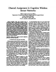
A. Simulations with Testbed Topologies We evaluate our algorithms on the topology of a physical indoor testbed in Bryan Hall of Washington University [1]. The testbed consists of 48 TelosB motes each equipped with a Chipcon CC2420 radio compliant with IEEE 802.15.4. At transmission power of 0 dBm, every node broadcasts 50 packets in a round-robin fashion. The neighbors record the sequence numbers of the packets they receive. This cycle is repeated for 5 rounds. Then every link with a higher than 80% PRR is considered reliable and drawn in Figure 2 (embedded on the floor plan of Bryan Hall). Using 12 channels,

Testbed topology (at transmission power of 0 dBm) in Bryan Hall

Varying deadlines. We generate flows in the network by randomly selecting the sources and destinations considering θ = 80% (i.e., 40% of the total nodes are sources while another 40% are destinations). The periods of the flows are randomly generated in range 26∼9 time slots. We generate 100 test cases and plot the acceptance ratios in Figure 3 by varying the deadlines of the flows (by changing α). For γ = 1 (Figure 3(a)), when α = 0.4, there are acceptable assignments in 55% test cases but PD is able to find an acceptable assignment only in 18% cases. Thus, the difference between the acceptance ratios of LS and PD is 0.37 when α = 0.4. For any α ≥ 0.4, the difference remains at least 0.14. For DM, this difference is 0.10 to 0.15. When γ = 2 (Figure 3(b)), the differences are 0.23 to 0.45 for PD, and 0.17 to 0.31 for DM. HS performs almost like an optimal algorithm in this setup since it selects good branches and uses a strong necessary condition to discard unnecessary branches (as explained in Section VI).

1 Acceptance ratio

Fig. 2.

worst, we omit any further comparison with PD. For every θ, we generate 100 test cases and show the performances in Figure 4. Since we use a sufficient schedulability test, there are cases when a priority assignment is not acceptable by the test but the flows may meet their deadlines if they are scheduled using that priority assignment. Therefore, every priority assignment generated by an algorithm is tested in simulation by scheduling all flows within their hyper-period. In the figure, each curve “sim” shows the fractions of test cases that have no deadline misses in simulations. When γ = 1 (Figure 4(a)), the difference between the acceptance ratios of LS and DM is always 0.02 to 0.11. Their difference in simulation is 0.02 to 0.05 when θ ≥ 60%. When γ = 2 (Figure 4(b)), their difference is 0.11 to 0.23 in acceptance ratio, and 0.02 to 0.16 in simulation. Here, HS performs like LS when γ = 1. When γ = 2, its acceptance ratio is 0.01 to 0.02 less than that of LS, if θ ≥ 80%.

Acceptance ratio

0.9 0.85

Fig. 4. Setup: m=12 θ=80% 6~9 T~=2

0 0.2

0.4

0.6 α

0.8

LS HS DM PD 1

(a) Acceptance ratio when γ = 1 0.8 0.6 0.4

Setup: m=12 θ=80% T~=26~9

LS HS DM PD

0.2 0 0.2

0.4

0.6 α

0.8

1

(b) Acceptance ratio when γ = 2 Fig. 3. Performance under varying deadlines

Varying sources and destinations. Now we vary θ resulting in different numbers of flows in the network. Since PD performs

Setup: α=1.0 m=12 6~9 T~=2

60

80

100

% Source or destination nodes (θ)

1

0.5

0 40

0.5

LS(sim) LS HS(sim) HS DM(sim) DM

(a) Acceptance ratio when γ = 1

1

Aceptance ratio

0.95

0.8 40

Acceptance ratio

we compare HS, LS, DM, and PD considering the Class-1 schedulability test presented in Section IV on this topology.

LS(sim) LS HS(sim) HS DM(sim) DM

Setup: α=1.0 m=12 6~9 T~=2

60

80

% Source or destination nodes (θ)

100

(b) Acceptance ratio when γ = 2 Performance under varying number of sources and destinations

B. Simulations with Random Topologies We test the scalability of our algorithms on random topologies of different number of nodes (N ). For every N , we generate 100 random networks, each with an edge-density (ρ) of 40%, i.e., with N (N −1)40/200 edges. PRR of each edge is randomly assigned between 0.80 and 1.0. In this setup, periods are in range 26∼11 slots to accommodate large networks. Here, we consider both the Class-1 schedulability test (Test 1) and the Class-2 schedulability test (Test 2) presented in Section IV. Starting with N = 30, we increase N as long as HS can find acceptable assignments and plot the performances in Figure 5. For γ = 1 (Figure 5(a)), HS is able to find an acceptable assignment in every case when N ≤ 110. When N > 110, there is a difference from 0.01 to 0.02 between LS and HS in both acceptance ratio and simulation. For γ = 2 (Figure 5(b)), the difference in both acceptance ratio and simulation is 0.01 to .02 when N > 50. The figures also indicate that the acceptance ratio with Test 2 is much lower than that with Test 1. For Test

0.8 0.6 0.4 0.2 0

LS−Test 1(sim) LS−Test 1 HS−Test 1(sim) HS−Test 1 LS−Test 2(sim) LS−Test 2

50

100 150 Number of nodes (N)

200

1

Setup: α=1.0 ρ=40% m=12 θ=80% T~=26~11

0.8 0.6

LS−Test 1(sim) LS−Test 1 HS−Test 1(sim) HS−Test 1 LS−Test 2(sim) LS−Test 2

0.4 0.2 0

(a) Acceptance ratio when γ = 1 Fig. 5.

50

100 Number of nodes (N)

150

(b) Acceptance ratio when γ = 2 Performance under varying network sizes

2 in this set up, there exists an acceptable assignment when N ≤ 150 and γ = 1 (Figure 5(a)), and when N ≤ 90 and γ = 2 (Figure 5(b)). This is because Test 2 is a less effective schedulability test compared to Test 1. However, both LS and HS are optimal for Test 2 (and we plot it only for LS). We abort LS if it cannot complete any test case in 10 minutes. Using Test 1, we have been able to record its performance when N ≤ 150 for γ = 1, and N ≤ 90 for γ = 2. With γ = 1, its average execution time remains within 5s when N ≤ 100, and increases sharply to 36s for N = 150 (Figure 5(c)). In contrast, HS takes 14s on average when N = 230 and γ = 1. When γ = 2, its average execution time is 15s when N = 150. If N > 150, HS cannot find an acceptable priority assignment for any test case. Using Test 2, the execution time of LS remains less than 5s (as long as there exists an assignment acceptable by Test 2). These results indicate that HS is an effective priority assignment algorithm as it is near-optimal and scales better than LS. VIII. R ELATED W ORKS For transmission scheduling in wireless sensor networks, schedulability analysis has been addressed in previous works [3], [8] considering the fixed priorities as given. For WirelessHART networks, convergecast scheduling for linear and tree [15], [17], [18] topologies, and real-time flow scheduling for arbitrary topologies [14] have been addressed in recent works. The schedulability analysis proposed in [13] assumes that the priorities of flows are given. None of these works addresses the priority assignment for real-time flows. Complementary to these works on scheduling for WirelessHART networks, we propose an optimal and a near-optimal priority assignment algorithm for real-time flows with fixed priorities. Alur et al. [4] have proposed a mathematical framework to model and analyze schedules using automata for WirelessHART networks. But their formal method approach can be computationally expensive making it suitable only for offline design. In contrast, our heuristic search is suitable for online admission control and adaptation, which is needed to handle both dynamic workloads and topology changes common in wireless networks. Moreover, our approach is tailored for fixed priority scheduling that is commonly adopted in real-time networks due to its simplicity and efficiency. IX. C ONCLUSION WirelessHART is an important standard for wireless sensoractuator networks that have increasing adoption in process

50 Execution time (second)

Setup: α=1.0 ρ=40% m=12 θ=80% 6~11 T~=2

Acceptance ratio

Acceptance ratio

1

40

Setup: α=1.0 ρ=40% m=12 θ=80% 6~11 T~=2

30

LS−Test 1(γ=2) LS−Test 1(γ=1) HS−Test 1(γ=2) HS−Test 1(γ=1) LS−Test 2(γ=2) LS−Test 2(γ=1)

20 10 0

50

100 150 Number of nodes (N)

200

(c) Execution time

industries. This paper is the first to address the priority assignment for real-time flows in WirelessHART networks. We have proposed an optimal algorithm based on local search and an efficient heuristic for priority assignment. Simulations on random networks and a sensor network testbed topology showed that the heuristic achieved near-optimal performance in terms of schedulability, while significantly outperforming traditional priority assignment policies for real-time systems. ACKNOWLEDGEMENT This research was supported by NSF under grants CNS0448554 (CAREER), CNS-1017701 (NeTS), and CNS0708460 (CRI). R EFERENCES [1] http://mobilab.wustl.edu/testbed. [2] WirelessHART specification, 2007. http://www.hartcomm2.org. [3] A BDELZAHER , T. F., P RABH , S., AND K IRAN , R. On real-time capacity limits of multihop wireless sensor networks. In RTSS ’04. [4] A LUR , R., D’I NNOCENZO , J OHANSSON , PAPPAS , AND W EISS , G. Modeling and analysis of multi-hop control network. In RTAS ’09. [5] AUDSLEY., N. C. On priority assignment in fixed priority scheduling. Information Processing Letters 79, 1 (2001). [6] B ERTOGNA , M., C IRINEI , M., AND L IPARI , G. Schedulability analysis of global scheduling algorithms on multiprocessor platforms. Parallel and Distributed Systems, IEEE Transactions on 20, 4 (2009), 553 –566. [7] C HEN , D., N IXON , M., AND M OK , A. WirelessHARTTM Real-Time Mesh Network for Industrial Automation. Springer, 2010. [8] C HIPARA , O., L U , C., AND ROMAN , G.-C. Real-time query scheduling for wireless sensor networks. In RTSS ’07. [9] DAVIS , R. I., AND B URNS , A. Priority assignment for global fixed priority pre-emptive scheduling in multiprocessor real-time systems. In RTSS ’09. [10] DAVIS , R. I., AND B URNS , A. Improved priority assignment for global fixed priority pre-emptive scheduling in multiprocessor real-time systems. Real-Time Syst. 47 (January 2011), 1–40. [11] G UAN , N., S TIGGE , M., Y I , W., AND Y U , G. New response time bounds for fixed priority multiprocessor scheduling. In RTSS ’09. [12] L IU , J. W. Real-time Systems. Prentice Hall, 2000. [13] S AIFULLAH , A., X U , Y., L U , C., AND C HEN , Y. End-to-end delay analysis for fixed priority scheduling in WirelessHART networks. In RTAS ’11. [14] S AIFULLAH , A., X U , Y., L U , C., AND C HEN , Y. Real-time scheduling for WirelessHART networks. In RTSS ’10. [15] S OLDATI , P., Z HANG , H., AND J OHANSSON , M. Deadline-constrained transmission scheduling and data evacuation in WirelessHART networks. In The European Control Conference 2009 (ECC ’09). [16] S ONG , J., M OK , A. K., C HEN , D., AND N IXON , M. Challenges of wireless control in process industry. In CRTES ’06. [17] Z HANG , H., O STERLIND , F., S OLDATI , P., V OIGT, T., AND J OHANS SON , M. Rapid convergecast on commodity hardware: Performance limits and optimal policies. In SECON ’10. [18] Z HANG , H., S OLDATI , P., AND J OHANSSON , M. Optimal link scheduling and channel assignment for convergecast in linear WirelessHART networks. In IEEE WiOpt (Seoul, Korea, Jun 2009).