RTSS2007 Robust Priority Assignment In Fixed Priority ... - CiteSeerX

Exact Quantification of the Sub-optimality of Uniprocessor Fixed Priority Pre-emptive Scheduling. Robert I. Davis, Thomas Rothvoß, Sanjoy K. Baruah, and Alan Burns Robert I. Davis ( ) Real-Time Systems Research Group, Department of Computer Science, University of York, York, UK. Email: [email protected] Thomas Rothvoß Ecole Polytechnique Federale de Lausanne, Institute of Mathematics, Station 8 - Bâtiment MA, CH-1015 Lausanne, Switzerland. Email: [email protected] Sanjoy K. Baruah Department of Computer Science, University of North Carolina, Chapel Hill, NC 27599-317, Carolina, USA. Email: [email protected] Alan Burns Real-Time Systems Research Group, Department of Computer Science, University of York, York, UK. Email: [email protected]

Keywords: Real-time Uniprocessor Fixed priority pre-emptive scheduling Earliest Deadline First (EDF) Suboptimality Processor speedup factor Constrained deadline Implicit deadline Omega constant

Abstract

1. Introduction

This paper examines the relative effectiveness of fixed priority pre-emptive scheduling in a uniprocessor system, compared to an optimal algorithm such as Earliest Deadline First (EDF). The quantitative metric used in this comparison is the processor speedup factor, equivalent to the factor by which processor speed needs to increase to ensure that any taskset that is schedulable according to an optimal scheduling algorithm can be scheduled using fixed priority pre-emptive scheduling, assuming an optimal priority assignment policy. For constrained-deadline tasksets where all task deadlines are less than or equal to their periods, the maximum value for the processor speedup factor is shown to be 1 / Ω ≈ 1.76322 , (where Ω is the mathematical constant defined by the transcendental equation ln(1 / Ω) = Ω , hence, Ω ≈ 0.567143 ). Further, for implicit-deadline tasksets where all task deadlines are equal to their periods, the maximum value for the processor speedup factor is shown to be 1/ln(2) ≈ 1.44270 . The derivation of this latter result provides an alternative proof of the well-known Liu and Layland result.

In this paper, we are interested in determining the largest factor by which the processing speed of a uniprocessor would need to be increased, such that any taskset, that was previously schedulable according to an optimal scheduling algorithm, could be guaranteed to be schedulable according to fixed priority pre-emptive scheduling, assuming an optimal priority assignment policy. We refer to this resource augmentation factor as the processor speedup factor (Kalyanasundaram and Pruhs, 1995). Analysis of fixed priority pre-emptive scheduling effectively began with Fineberg and Serlin (1967) who considered priority assignment for two independent periodic tasks with deadlines equal to their periods and bounded execution times. They noted that if the task with the shorter period is assigned the higher priority, then the taskset is guaranteed to be schedulable provided that its total utilisation1 U ≤ 2( 2 − 1) ≈ 82.8% . The above result was generalised by Liu and Layland 1

The utilisation of a task is defined as its execution time divided by its period. The utilisation of a taskset is the sum of the utilisations of its tasks.

1

defined by the transcendental equation ln(1 / Ω) = Ω , hence, Ω ≈ 0.567143 ). The significance of our main result is to provide a bound, analogous to the seminal schedulability result of Liu and Layland (1973) ( U ≤ ln(2) ≈ 69.3% ), that applies to constrained-deadline rather than implicitdeadline tasksets. An exact condition for the schedulability of a constrained-deadline taskset under an optimal preemptive uniprocessor scheduling algorithm, such as EDF (Dertouzos, 1974), is that a quantity referred to as the processor LOAD (see Section 2.4) does not exceed the capacity of the processor (i.e. LOAD ≤ 1 ) (Baruah et al. 1990a, 1990b). The processor speedup factor derived in this paper shows that every constrained-deadline taskset with LOAD ≤ Ω ≈ 0.567143 is guaranteed to be schedulable according to fixed priority pre-emptive scheduling using deadline-monotonic priority assignment. While the results presented in this paper are mainly theoretical, they also have practical utility in enabling system designers to quantify the maximum penalty for using fixed priority pre-emptive scheduling in terms of the additional processing capacity required. This performance penalty can then be weighed against other factors such as implementation overheads when considering which scheduling algorithm to use.

(1973) who considered the pre-emptive scheduling of synchronous2 tasksets comprising independent periodic tasks, with bounded execution times, and deadlines equal to their periods. We refer to such tasksets as implicit-deadline tasksets. Liu and Layland (1973) showed that rate monotonic (RM) priority ordering is the optimal fixed priority assignment policy for implicitdeadline tasksets, and that using rate monotonic priority ordering, fixed priority pre-emptive scheduling can schedule any implicit-deadline taskset with a total utilisation U ≤ ln(2) ≈ 69.3% . Liu and Layland (1973) also showed that Earliest Deadline First (EDF) is an optimal dynamic priority scheduling algorithm for implicit-deadline tasksets, and that EDF can schedule any such taskset with a total utilisation U ≤ 1 . Dertouzos (1974) showed that EDF is in fact an optimal pre-emptive uniprocessor scheduling algorithm, in the sense that if a schedule exists for a taskset, then the schedule produced by EDF will also be feasible. Combining the result of Dertouzos (1974) with the results of Liu and Layland (1973) for both EDF and fixed priority pre-emptive scheduling, we can see that the processor speedup factor required to guarantee that fixed priority pre-emptive scheduling can schedule any feasible implicit-deadline taskset is 1 / ln(2) ≈ 1.44270 . In the 1980’s, and early 1990’s research into realtime scheduling focused on constrained-deadline tasksets; synchronous tasksets comprising independent sporadic tasks with bounded execution times, known minimal inter-arrival times or periods, and deadlines constrained to be less than or equal to their periods. Leung and Whitehead (1982) showed that deadline monotonic3 (DM) priority ordering is the optimal fixed priority ordering for constrained-deadline tasksets. Exact fixed priority schedulability tests for constraineddeadline tasksets were introduced by Joseph and Pandya (1986), Lehoczky et al. (1989), and Audsley et al. (1993). Exact EDF schedulability tests for constraineddeadline tasksets were introduced by Baruah et al. (1990a, 1990b). Recently, Baruah and Burns (2008) showed that the processor speedup factor required for fixed priority preemptive scheduling of constrained-deadline tasksets is upper-bounded by 2 and lower-bounded by 1.5. In this paper, we prove that the exact processor speedup factor required for fixed priority pre-emptive scheduling of constrained-deadline tasksets is 1 / Ω ≈ 1.76322 (where Ω is the mathematical constant

1.1. Related work on average case suboptimality This paper examines the sub-optimality of fixed priority pre-emptive scheduling in the worst-case, other research has examined its behaviour in the average-case. Lehoczky et al. (1989) introduced the breakdown utilisation metric: A taskset is randomly generated, and then all task execution times are scaled until a deadline is just missed. The utilisation of the scaled taskset gives the breakdown utilisation. Lehoczky et al. (1989) showed that the average breakdown utilisation, for implicit-deadline tasksets of large cardinality under fixed priority pre-emptive scheduling is approximately 88%, corresponding to a penalty of approximately 12% of processing capacity with respect to an optimal algorithm such as EDF. Bini and Buttazzo (2005) showed that breakdown utilisation suffers from a bias which tends to penalise fixed priority scheduling by favouring tasksets where the utilisation of individual tasks is similar. Bini and Buttazzo (2005) introduced the optimality degree metric, defined as the number of tasksets in a given domain that are schedulable according to some algorithm A divided by the number that are schedulable according to an optimal algorithm. Using this metric, they showed that the penalty for using fixed priority-pre-emptive scheduling for implicit-deadline tasksets is typically

2

A taskset is synchronous if all of its tasks share a common release time. 3 Deadline monotonic priority ordering assigns priorities in order of task deadlines, such that the task with the shortest deadline is given the highest priority.

2

time divided by its period ( U i = Ci / Ti ). The total utilisation U, of a taskset is the sum of the utilisation of all of its tasks. The following assumptions are made about the behaviour of the tasks: o The arrival times of the tasks are independent and hence the tasks may share a common release time. o Each task is released (i.e. becomes ready to execute) as soon as it arrives. o The tasks are independent and so cannot block each other from executing by accessing mutually exclusive shared resources, with the exception of the processor. o The tasks do not voluntarily suspend themselves. A task is said to be ready if it has outstanding computation and so is awaiting execution by the processor. A taskset is said to be schedulable with respect to some scheduling algorithm and some system, if any sequence of invocations generated by the taskset can be scheduled on the system by the scheduling algorithm without any deadlines being missed. Under Earliest Deadline First (EDF) scheduling, at any given time, the ready task (invocation) with the earliest absolute deadline is executed by the processor. In contrast, under fixed priority pre-emptive scheduling, at any given time, the highest priority ready task is executed by the processor. We assume that when a taskset is scheduled according to fixed priorities, these priorities are assigned according to deadline-monotonic priority ordering, as deadline-monotonic is known to be the optimal priority ordering for both constrained-deadline (Leung and Whitehead, 1982) and implicit-deadline tasksets (Liu and Layland, 1973). We note that deadline-monotonic is the optimal priority ordering in the sense that there are no constrained-deadline tasksets that are schedulable according to fixed priority pre-emptive scheduling using any other priority ordering that are not also schedulable using deadline-monotonic priority ordering. This does not however mean that deadline-monotonic fixed priority pre-emptive scheduling is an optimal scheduling algorithm for such tasksets. (The definition of scheduling algorithm optimality is given below).

significantly lower than that assumed by determining the average breakdown utilisation.

1.2. Organisation The remainder of this paper is organised as follows. Section 2 describes the system model and notation used, recapitulates exact schedulability analysis for both fixed priority and EDF scheduling, and provides a number of key definitions. Section 3 derives the structure and parameters of a speedup-optimal taskset (defined in Section 2) for the class of tasksets with constrained deadlines. Section 4 derives the exact processor speedup factor required for constrained-deadline tasksets of arbitrary cardinality, under fixed priority pre-emptive scheduling. Appendix A complements Section 4 by providing an upper bound on the processor speedup factor for tasksets of cardinality n which improves upon the general result for arbitrary n. Section 5 extends the results of Sections 3 and 4 to implicit-deadline tasksets, providing an alternative proof of the seminal results of Fineberg and Serlin (1967) and Liu and Layland (1973). Finally, Section 6 concludes with a summary of the results.

2. Scheduling analysis

model

and

schedulability

In this section, we outline the scheduling model, notation and terminology used in the rest of the paper. We then recapitulate the exact schedulability analysis for both fixed priority pre-emptive scheduling and EDF scheduling. Finally, we provide a number of definitions that are used in subsequent analysis and illustrate the fundamental concepts with an example.

2.1. Scheduling model, terminology and notation In this paper, we consider the pre-emptive scheduling of a set of tasks (or taskset) on a uniprocessor. Each taskset comprises a static set of n tasks ( τ 1 ..τ n ), where n is a positive integer. We assume that the index i of task τ i also represents the task priority used in fixed priority pre-emptive scheduling, hence τ 1 has the highest fixed-priority, and τ n the lowest. Each task τ i is characterised by its bounded worstcase execution time Ci , minimum inter-arrival time or period Ti , and relative deadline Di . Each task τ i therefore gives rise to a potentially infinite sequence of invocations, each of which has an execution time upper bounded by C i , an arrival time at least Ti after the arrival of its previous invocation, and an absolute deadline Di time units after its arrival. In a constrained-deadline taskset, all tasks have Di ≤ Ti , while in an implicit-deadline taskset, all tasks have Di = Ti . The utilisation U i , of a task is given by its execution

2.2. Feasibility and optimality A taskset is said to be feasible with respect to a given system model if there exists some scheduling algorithm that can schedule the taskset on that system without missing any deadlines. Note, in this paper, we are primarily interested in a reference system model that consists of a pre-emptive uniprocessor with unit

3

Iteration starts with an initial value wi0 , typically wi0 = Ci , and ends when either wim+1 = wim in which case the worst-case response time Ri , is given by wim+1 , or when wim+1 > Di in which case the task is unschedulable. Note, the values of wim are monotonically nondecreasing with respect to the iteration count m (Tindell, 1994), and so the fixed point iteration is guaranteed to converge to the worst-case response time Ri , provided that the overall taskset utilisation is less than or equal to 1, and the initial value wi0 is a lower bound on Ri (Sjodin and Hansson, 1998). Response Time Analysis, as embodied in Equation (1), thus provides an exact schedulability test for constrained-deadline tasksets scheduled under fixed priority pre-emptive scheduling. In subsequent analysis, we also make use of the concept of a priority level-i idle period. This is defined as an interval of time [t 3 , t 4 ) of length greater than zero, during which no tasks are ready to execute at priority i or higher strictly before the end of the idle period at t 4 .

processing speed. A scheduling algorithm is said to be optimal with respect to a system model and a tasking model if it can schedule all of the tasksets that comply with the tasking model and are feasible on the system. We note that EDF is known to be an optimal preemptive uniprocessor scheduling algorithm for constrained-deadline tasksets compliant with the tasking model described in Section 2.1 (Dertouzos, 1974). Least Laxity First is another such optimal algorithm (Mok, 1983).

2.3. Exact schedulability analysis for FPPS In this section, we give a brief summary of Response Time Analysis (Audsley et al., 1993) used to provide an exact schedulability test for fixed priority pre-emptive scheduling on a uniprocessor. First, we introduce the concepts of worst-case response time, critical instant, and busy periods, which are fundamental to this form of analysis. For a given taskset scheduled under fixed priority pre-emptive scheduling, the worst-case response time Ri of task τ i is given by the longest possible time from release of the task until it completes execution. Thus task τ i is schedulable if and only if Ri ≤ Di , and the taskset is schedulable if and only if ∀i Ri ≤ Di . A critical instant for task τ i , refers to a time at which task τ i is released, and the pattern of releases of other tasks in the taskset is such that task τ i exhibits its worst-case response time (Liu and Layland, 1973). Under fixed priority pre-emptive scheduling, for independent tasks with constrained-deadlines, a critical instant occurs when all of the tasks are released simultaneously, and then subsequent task releases occur as early as possible. The term priority level-i busy period refers to a period of time [t1 , t 2 ) during which the processor is busy executing computation at priority i or higher, that was released at the start of the busy period at t1 , or during the busy period but strictly before its end at t 2 . Under fixed priority pre-emptive scheduling, the worst-case response time Ri of a constrained-deadline task τ i corresponds to the length of the longest priority level-i busy period, which starts at a critical instant. The busy period comprises two components, the execution time Ci of the task itself, and so called interference, equal to the time for which task τ i is prevented from executing by higher priority tasks. The length of the busy period wi , can be computed using the following fixed point iteration (Audsley et al., 1993), with the summation term giving the interference due to the set of higher priority tasks hp(i). ⎡ wm ⎤ wim +1 = Ci + ∑ ⎢ i ⎥C j (1) ∀j∈hp (i ) ⎢ T j ⎥

2.4. Exact schedulability analysis for EDF The schedulability of a constrained-deadline taskset under EDF can be determined via the processor demand bound function h(t) given below: n ⎛⎢ t − Di ⎥ ⎞⎟ (2) +1 C h(t ) = ∑ ⎜ ⎢ ⎜ T ⎥ ⎟ i i ⎦ i =1 ⎝ ⎣ ⎠ Baruah et al (1990a, 1990b) showed that a taskset is schedulable under EDF if and only if a quantity referred to as the processor LOAD is ≤ 1 where the processor LOAD is defined as follows: ⎛ h(t ) ⎞ LOAD = max⎜ (3) ⎟ ∀t ⎝ t ⎠ Further, they showed that the maximum value of h(t ) / t occurs for some value of t in the interval (0, L) , where L is defined as follows, thus limiting the number of values of t that need to be checked to determine schedulability. ⎛ U ⎞⎞ ⎛ L = max⎜⎜ D1 , D2 ,...Dn, max⎜ (Ti − Di ) ⎟⎟ ∀i ⎝ 1 − U ⎠ ⎟⎠ ⎝ Significant developments have been made, extending the scope of the schedulability tests given in Equations (1) and (2); however, these basic forms are sufficient for the purposes of this paper.

2.5. Definitions Our analysis uses the concept of uniform processors. We refer to two processors as uniform (or similar) if the rate of execution of any task on each of the two processors depends only on the difference in clock speed of the processors. Thus a processor of speed 1 takes exactly twice the time to execute any given task as a

4

factor by which the execution times of a set of tasks, that are only just schedulable according to fixed priority preemptive scheduling (i.e. with α S = 1 ), can be increased, and yet the taskset remain schedulable according to an optimal scheduling algorithm (e.g. EDF).

similar processor of speed 2. Definition 1: Let Ψ be a taskset that is feasible (i.e. schedulable according to an optimal scheduling algorithm) on a processor of speed 1. Now assume that f (Ψ ) is the lowest speed of any similar processor that will schedule taskset Ψ using scheduling algorithm A. The processor speedup factor f A for scheduling algorithm A is given by the maximum processor speed required to schedule any such taskset Ψ . f A = max( f (Ψ ) )

Corollary 1: The processor speedup factor for fixed priority pre-emptive scheduling is equal to the largest EDF scaling factor f S of any taskset with a fixed priority scaling factor α S = 1 . Definition 3: A taskset is said to be speedup-optimal if it has the largest EDF scaling factor f S of any taskset that is only just schedulable according to fixed priority pre-emptive scheduling ( α S = 1 ).

∀Ψ

For any scheduling algorithm A, we have4 f A ≥ 1 , with smaller values of f A indicative of a more effective scheduling algorithm, and f A = 1 implying that A is an optimal algorithm. In the remainder of the paper, unless otherwise stated, when we refer to the processor speedup factor, we mean the processor speedup factor for fixed priority pre-emptive scheduling using an optimal priority assignment policy. The problem of determining this processor speedup factor can be addressed from two different perspectives: 1. Speeding up a processor to guarantee that a taskset that is already schedulable under an optimal algorithm becomes schedulable under fixed priority pre-emptive scheduling. 2. Slowing down a processor and hence scaling up the execution times of a set of tasks that are only just schedulable according to fixed priority preemptive scheduling, until they are only just schedulable according to an optimal algorithm. Our analysis addresses the problem from the latter perspective. For a taskset S to be schedulable according to fixed priorities, let α S ( α S ≥ 1 ) be the largest factor by which all of the execution times of the tasks in S can be scaled and the taskset remain schedulable under fixed priority pre-emptive scheduling. We refer to α S as the fixed priority scaling factor. Similarly, let f S ( f S ≥ 1 ) be the largest factor by which all of the execution times of the tasks in S can be scaled and the taskset remain schedulable under EDF scheduling. We refer to f S as the EDF scaling factor. We now give an alternative but equivalent definition of the processor speedup factor. (In Appendix B, we prove that Definition 2 is equivalent to Definition 1).

Corollary 2: The processor speedup factor is equal to the EDF scaling factor f S of a speedup-optimal taskset.

We note that the value of the processor speedup factor and the parameters of speedup-optimal tasksets depend on the class of tasksets considered. For example the class of implicit-deadline tasksets of cardinality two has a smaller processor speedup factor than the class of constrained-deadline tasksets with arbitrary cardinality, and different speedup-optimal tasksets. In the remainder of the paper, when the terms processor speedup factor and speedup-optimal taskset are used, the class of tasksets considered is explicitly stated only when this is not readily apparent from the context. Definition 4: A constraining task is defined as a task that cannot have its execution time increased without missing its deadline, and hence the taskset becoming unschedulable. Corollary 3: Under fixed priority pre-emptive scheduling, for a constraining task τ i , the interval [0, Di ) , starting with a critical instant at t=0, where all tasks are released simultaneously and then subsequently released as early as possible, contains no priority level-i idle time. Corollary 4: Any taskset S with α S = 1, has at least one constraining task.

2.6. Example The concepts introduced in this section can be illustrated by means of an example. Consider an implicit-deadline taskset S comprising the two tasks defined in Table 1. The parameters of these tasks appear to have some rather unusual values; however, this is because they have been chosen so that the taskset is speedup-optimal with respect to the class of implicit-

Definition 2: The processor speedup factor for fixed priority pre-emptive scheduling is the maximum scaling 4

The set of all tasksets that are feasible on a processor of speed 1 contains tasksets that fully utilise the processor. For example Ci = Di = Ti = 1. Given such a taskset, the processor speedup factor for any scheduling algorithm cannot be less than 1.

5

cardinality two is 1/(2( 2 - 1)) ≈ 1.207107 . Note, in Section 5 we prove this result independently without using the utilisation bound of Fineberg and Serlin (1967).

deadline tasksets with cardinality two. The total utilisation of the taskset is 2( 2 - 1) ≈ 0.828427 . Table 1 Task

Ci

Di = Ti

Ui

Ri

3. Speedup-optimal tasksets

τ1

1

1+ 2

2 -1

1

2

2+ 2

2 -1

1+ 2

In this section, we derive the structure and parameters of speedup-optimal tasksets for the class of tasksets with constrained deadlines ( Di ≤ Ti ). Before considering tasksets of arbitrary cardinality, we first present results for tasksets comprising just two tasks. The derivation of this result provides the intuition for the general case. Theorem 1 describes the parameters of a taskset that is speedup-optimal with respect to all constraineddeadline tasksets of cardinality two. Theorem 2 describes the parameters of a taskset that is speedup-optimal with respect to all constraineddeadline tasksets. The proofs of Theorems 1 and 2 rely on Lemmas 18. The basic method and intuition behind the proofs of Lemmas 1-8 is given after the Theorems, this followed by the Lemmas and their specific proofs. Note that in the various discussions, theorems, lemmas, and proofs in this and subsequent sections, fixed priority pre-emptive scheduling should be assumed unless otherwise stated.

τ2

D1 1

√2

D2 1

T1

T2

Figure 1

Figure 1 illustrates the execution of the tasks under fixed priority pre-emptive scheduling, starting at a critical instant. Note that although the worst-case response time of task τ 2 is significantly less than its deadline D2 , τ 2 is a constraining task; since any increase in its execution time will cause its deadline to be missed. Taskset S has a fixed priority scaling factor α S = 1 , as increasing the execution times of the tasks by any factor greater than 1 would result in the taskset becoming unschedulable. As EDF can schedule any implicit deadline taskset with utilisation no greater than 100%, we can scale the execution times of tasks τ 1 and τ 2 by a factor of 1/(2( 2 - 1)) , and the resulting taskset, with 100% utilisation, will be just schedulable under EDF. The EDF scaling factor f S for taskset S is therefore 1/(2( 2 - 1)) ≈ 1.207107 . We note that the parameters of the tasks in taskset S have been carefully selected so that the utilisation of this taskset matches the Fineberg and Serlin (1967) utilisation bound of 2( 2 - 1) for implicit-deadline tasksets of cardinality two. As all tasksets with cardinality two and utilisation less than or equal to this bound are known to be schedulable, any taskset with utilisation strictly less than the bound must have a fixed priority scaling factor that is strictly greater than 1. Hence taskset S has the minimum utilisation of any taskset that is only just schedulable according to fixed priority pre-emptive scheduling ( α S = 1 ). Taskset S therefore exhibits the largest EDF scaling factor f S of any taskset that has α S = 1 , and hence is a speedupoptimal taskset. The processor speedup factor is equal to the EDF scaling factor f S of a speedup-optimal taskset, hence the processor speedup factor for fixed priority preemptive scheduling of implicit deadline tasksets of

Theorem 1: For constrained-deadline tasksets of cardinality two, there is a speedup-optimal taskset V, with α V = 1, which has the following parameters: τ 1 : C1 = 1 , D1 = T1 = 1 + X τ 2 : C 2 = X , D2 = 2 + X , T2 = ∞ Where X ≥ 0 is some as yet unknown value for the execution time of τ 2 . Note that the execution time of τ 1 in Theorem 1 has been normalised to 1 and the task periods and deadlines adjusted accordingly5. There is one free variable in the taskset parameters, that is X, the execution time of task τ 2 . This taskset is illustrated in Figure 2.

Figure 2 Proof: Proof follows directly from Lemmas 1 to 8, specifically: 5

All of the task parameters can be scaled linearly without changing the fundamental properties of the taskset.

6

o o o o o o o

o

□

τ 2 must be a constraining task, with the longest deadline and the lowest priority (Lemma 1). τ 2 must have an infinite period (Lemma 2). t = D2 must be the start of an idle period (Lemma 3). T1 < D2 (Lemma 4) D1 = T1 (Lemma 5). T1 > D2 / 2 (Lemma 6). Following a critical instant, τ 2 must execute continuously from when it first starts execution until it completes (Lemma 7). The parameters of task τ 1 must comply with D1 = T1 = C1 + C 2 = 1 + X (Lemma 8).

o

The task parameters must comply with the following equation (Lemma 8): ∀i ≠ n Di = Ti = ∑ C j + ∑ C j ∀j

∀j∈hp (i )

Finally, applying Lemma 9 repeatedly shows that slicing the total amount of higher priority task execution time into an infinite number of tasks each with an infinitesimal execution time leads to a speedup-optimal taskset6 □

3.1. Method and intuition The problem of determining the parameters of a speedup-optimal taskset for the class of tasksets with constrained-deadlines is solved by breaking it down into a series of basic steps corresponding to Lemmas 1 to 8. At each step, we start with a set Z of tasksets, where Z is known to contain at least one speedup-optimal taskset. We then place a condition on the task parameters which selects a subset Y of the tasksets in Z ( Y ⊆ Z ). We then prove that for every taskset S that is in Z but is not a member of Y ( S ∈ Z ∩ Y c , where Y c is the complement of Y), there is a taskset V ∈ Y that has an EDF scaling factor fV at least as large as that of taskset S ( f V ≥ f S ). Hence we show that the reduced set Y also contains at least one speedup-optimal taskset. Lemmas 1-8 are proved by contradiction. They work in the following way: First we assume (for contradiction) that there is a taskset S ∈ Z ∩ Y c with an EDF scaling factor strictly larger than that of any taskset in Y. We then show that this cannot be the case, by transforming taskset S into another taskset V ∈ Y which we show has an EDF scaling factor at least as large as that of S ( f V ≥ f S ). This contradicts the original assumption. It follows that there are no tasksets in Z ∩ Y c that have an EDF scaling factor strictly greater than the maximum EDF scaling factor of any task in Y. As Z was known to contain at least one speedup-optimal taskset (with the maximum EDF scaling factor), then it follows that there must be at least one taskset in Y that has the maximum EDF scaling factor, and so is a speedup-optimal taskset, which proves the Lemma. Lemma 1 starts with Z representing the set of all tasksets that are just schedulable according to fixed priority pre-emptive scheduling. By definition, this set contains at least one speedup-optimal taskset. Once

Theorem 2: For constrained-deadline tasksets with arbitrary cardinality, there is a speedup-optimal taskset V, with α V = 1, which has the following parameters: Taskset V has an infinite number of tasks and is expressed as the limit of the following taskset as n→∞. ∀i ≠ n Di = Ti = 1 + X + (i − 1) /( n − 1) Ci = 1 /( n − 1) C n = X , Dn = 2 + X , Tn = ∞ (12) Where X ≥ 0 is some as yet unknown value for the execution time of τ n . Note that in Theorem 2, the total higher priority task execution time has again been normalised to 1 and the task periods and deadlines adjusted accordingly. There is one free variable in the taskset parameters, that is X, the execution time of task τ n . This taskset is illustrated in Figure 3.

Figure 3 Proof: Proof follows directly from Lemmas 1 to 9, specifically: o τ n must be a constraining task, with the longest deadline and the lowest priority (Lemma 1). o τ n must have an infinite period (Lemma 2). o t = Dn must be the start of an idle period (Lemma 3). o ∀i ≠ n Ti < Dn (Lemma 4) o ∀i ≠ n Di = Ti (Lemma 5). o ∀i ≠ n Ti > Dn / 2 (Lemma 6). o Following a critical instant, τ n must execute continuously from when it first starts execution until it completes (Lemma 7).

6

Strictly speaking, a speedup optimal taskset does not exist for the case of tasksets with arbitrary cardinality, in the same way that a largest integer does not exist for the infinite set of all integers. The concept of a speedup optimal taskset is however extremely useful in understanding processor speedup factors. In Theorem 2 we therefore express the speedup optimal taskset in terms of the limit of a taskset as its cardinality approaches infinity, and refer to it in subsequent text as if it does exist. We note that in practice, all real-time systems have a finite number of tasks, and speedup optimal tasksets exist for any class of tasksets with cardinality limited by a finite value.

7

Lemma 1 is proven, we know that the subset Y ⊆ Z contains at least one speedup-optimal taskset. Each subsequent lemma starts by setting Z equal to the subset Y defined by the previous lemma; hence multiple conditions are applied resulting in a constrained subset that is known to contain at least one speedupoptimal taskset. At the end of Lemmas 1-8, this allows for just one free variable X among the taskset parameters, aside from the number of tasks which is addressed by Lemma 9. By virtue of Lemmas 1-9, Theorems 1 and 2 define speedup-optimal tasksets sufficiently well for subsequent analysis of the exact processor speedup factor in Section 4. In a number of the lemmas, we make use of the concept of a sustainable change. A change to the parameters of the tasks in a schedulable taskset is said to be sustainable (Baruah and Burns, 2006) if following that change the taskset is guaranteed to remain schedulable. Baruah and Burns (2006) showed that under both EDF and fixed priority pre-emptive scheduling, increases in task periods, increases in task deadlines, and decreases in task execution times are all sustainable changes.

EDF, hence f V ≥ f S . This contradicts our original assumption, hence there are no tasksets in Z ∩ Y c that have an EDF scaling factor strictly greater than the maximum EDF scaling factor of any taskset in Y, and so there must be at least one speedup-optimal taskset in Y □ Lemma 2: Let Z be the set Y defined by Lemma 1, and Y be redefined as follows: Y ⊆ Z such that every taskset in Y has a lowest priority task τ n with an infinite period. The set Y contains at least one speedup-optimal taskset. Proof: We assume (for contradiction) that there is a taskset S ∈ Z ∩ Y c that has an EDF scaling factor f S strictly greater than that of any taskset in Y. We now create a new taskset V from taskset S, by increasing the period of task τ n to infinity. Taskset V has α V = 1, as schedulability of τ n under fixed priority pre-emptive scheduling is independent of its period Tn provided that Dn ≤ Tn (see Equation (1)), hence V ∈ Y . Increasing the period of any task is a sustainable change under fixed priority and EDF scheduling and so taskset V, scaled by a factor of f S is schedulable under EDF, hence f V ≥ f S . This contradicts our original assumption, hence there are no tasksets in Z ∩ Y c that have an EDF scaling factor strictly greater than the maximum EDF scaling factor of any taskset in Y, and so there must be at least one speedup-optimal taskset in Y □

3.2. Lemmas 1-9 The following lemmas are applicable to the class of tasksets with constrained deadlines. Lemma 1: Let Z be the set of all (constrained-deadline) tasksets that are just schedulable according to fixed priority pre-emptive scheduling ( α S = 1 for all the tasksets in Z). By definition, this set contains at least one taskset that is speedup-optimal with respect to the class of tasksets with constrained deadlines. Let Y ⊆ Z such that every taskset in Y has a single constraining task, and that task has the lowest priority, and hence the longest deadline. The set Y contains at least one speedupoptimal taskset.

Lemma 3: Let Z be the set Y defined by Lemma 2, and Y be redefined as follows: Y ⊆ Z such that every taskset in Y has a priority level-(n-1) idle period starting at time t = Dn , following a critical instant at time t = 0, when all of the tasks are released simultaneously, and are then released again as early as possible. Stated otherwise, all of the task execution released in the interval [0, Dn ) is completed by Dn , and no task of priority higher than n is released at time Dn . The set Y contains at least one speedup-optimal taskset.

Proof: We assume (for contradiction) that there is a taskset S ∈ Z ∩ Y c that has an EDF scaling factor f S strictly greater than that of any taskset in Y. By Corollary 4, taskset S contains at least one constraining task. Let task τ i ( i ≠ n) be the highest priority constraining task in S . (Note, τ n cannot be the highest priority constraining task in S, otherwise S would be a member of Y). We now create a new taskset V by removing all tasks of lower priority than i from S. As the lowest priority task in V is a constraining task, α V = 1, and hence V ∈ Y . Further, the tasks in V are a subset of the tasks in S. Removing a task is equivalent to decreasing its execution time to zero, and decreasing the execution time of any task is a sustainable change under both fixed priority and EDF scheduling. Taskset V, scaled by a factor of f S is therefore schedulable under

Proof: We assume (for contradiction) that there is a taskset S ∈ Z ∩ Y c that has an EDF scaling factor f S strictly greater than that of any taskset in Y. For taskset S, with a critical instant at time t = 0, time t = Dn is not the start of a priority level-(n-1) idle period, otherwise S would be a member of Y. Let the next such idle period start at some later time t = Dn′ > Dn . We now create a new taskset V from taskset S by increasing the deadline of τ n to Dn′ . We refer to the modified task as τ n′ . As τ n′ is a constraining task, taskset V has α V = 1 and hence V ∈ Y . Increasing the deadline of any task is a sustainable change under fixed priority and EDF scheduling and so taskset V, scaled by a factor of f S is schedulable under

8

EDF, hence f V ≥ f S . This contradicts our original assumption, hence there are no tasksets in Z ∩ Y c that have an EDF scaling factor strictly greater than the maximum EDF scaling factor of any taskset in Y, and so there must be at least one speedup-optimal taskset in Y □

EDF, hence f V ≥ f S . This contradicts our original assumption, hence there are no tasksets in Z ∩ Y c that have an EDF scaling factor strictly greater than the maximum EDF scaling factor of any taskset in Y, and so there must be at least one speedup-optimal taskset in Y □

Lemma 4: Let Z be the set Y defined by Lemma 3, and Y be redefined as follows: Y ⊆ Z such that every taskset in Y has task periods such that ∀i ≠ n Ti < Dn . The set Y contains at least one speedup-optimal taskset.

We note that the transformation detailed in the proof of Lemma 5 may result in changes to the order of task deadlines with respect to task priority. We assume that if this is the case, then the task priorities are altered so that they are once again in deadline monotonic priority order. We note that this does not affect taskset schedulability as deadline monotonic priority ordering is known to be optimal (Leung and Whitehead, 1982), and the taskset remains schedulable with its original priority ordering. Further, Lemma 4, shows that ∀i ≠ n Ti < Dn , hence after the above transformation, ∀i ≠ n Di < Dn , so task τ n remains the lowest priority and constraining task.

Proof: We assume (for contradiction) that there is a taskset S ∈ Z ∩ Y c that has an EDF scaling factor f S strictly greater than that of any taskset in Y. Let τ i be a task in taskset S that has Ti ≥ Dn . We now create a new taskset V from taskset S by removing each such task τ i with Ti ≥ Dn , and increasing the execution time of τ n by Ci (to form task τ n′ ). As there was only one invocation of each such task τ i in the interval [0, Dn ) , the same amount of computation remains in this interval, hence τ n′ is a constraining task and α V = 1, hence V ∈ Y . As τ n′ has an infinite period (due to the constraints placed on the tasksets in set Z by Lemma 2) and a deadline not less than that of τ i (due to the constraints placed on the tasksets in the set Z by Lemma 1), then the processor demand function h(t ) for taskset V is never larger than that for taskset S. Taskset V scaled by a factor of f S is therefore schedulable under EDF, hence f V ≥ f S . This contradicts our original assumption, hence there are no tasksets in Z ∩ Y c that have an EDF scaling factor strictly greater than the maximum EDF scaling factor of any taskset in Y, and so there must be at least one speedup-optimal taskset in Y □

Lemma 6: Let Z be the set Y defined by Lemma 5, and Y be redefined as follows: Y ⊆ Z such that every taskset in Y has task periods such that ∀i ≠ n Ti > Dn / 2 . The set Y contains at least one speedup-optimal taskset. Proof: We assume (for contradiction) that there is a taskset S ∈ Z ∩ Y c that has an EDF scaling factor f S strictly greater than that of any taskset in Y. Let τ i be a task in S that has Ti ≤ Dn / 2 . We now create a new taskset V from taskset S by transforming the parameters of each such task τ i (to form task τ i′ ) as follows. Ci′ = mCi , Di′ = Ti′ = mTi where m = ⎣Dn / Ti ⎦ . As Ti ≤ Dn / 2 we have Dn ≥ Ti′ ≥ Dn / 2 . We note that this transformation may result in changes to the order of task deadlines with respect to task priority. We assume that if this is the case, then the task priorities are altered so that the tasks are once again in deadline monotonic priority order. Note that τ n remains the lowest priority task. Following the above transformation, the amount of execution time released by τ i′ in the interval [0, Dn ) cannot be less than that released by τ i , hence taskset V has α V ≤ 1 . (We consider the fact that taskset V may now be unschedulable according to fixed priority scheduling (i.e. α V < 1 ) later in the proof). Considering EDF scheduling, the contribution to the processor demand function from each original task τ i (with Di = Ti ) is given by: ⎢t ⎥ hi (t ) = ⎢ ⎥Ci (4) ⎣ Ti ⎦

Lemma 5: Let Z be the set Y defined by Lemma 4, and Y be redefined as follows: Y ⊆ Z such that every taskset in Y has task periods and deadlines such that ∀i ≠ n Di = Ti . The set Y contains at least one speedup-optimal taskset. Proof: We assume (for contradiction) that there is a taskset S ∈ Z ∩ Y c that has an EDF scaling factor f S strictly greater than that of any taskset in Y. Let τ i be a task in taskset S that has Di < Ti . We now create a new taskset V from taskset S by increasing the deadline of each such task τ i , to form task τ i′ with Di′ = Ti . The total execution time in [0, Dn ) remains the same, and so τ n remains a constraining task and so α V = 1, hence V ∈ Y . Increasing the deadline of any task is a sustainable change under fixed priority and EDF scheduling and so taskset V, scaled by a factor of f S is schedulable under

Similarly, the contribution to the processor demand function from each transformed task τ i′ is given by:

9

As none of the above six steps can decrease the EDF scaling factor of taskset V, we have f V ≥ f S . This contradicts our original assumption, hence there are no tasksets in Z ∩ Y c that have an EDF scaling factor strictly greater than the maximum EDF scaling factor of any taskset in Y, and so there must be at least one speedup-optimal taskset in Y □

⎢ t ⎥ hi′ (t ) = ⎢ (5) ⎥ mCi ⎣ mTi ⎦ Equations (4) and (5) are both monotonically nondecreasing functions of t. hi (t ) is zero for t < Ti , and only increases in value at times t = gTi , for integer values of g. At these times, hi (t ) = gCi . hi′(t ) is zero for t < mTi , and only increases in value at times t = kmTi , for integer values of k. At these times, hi′ (t ) = kmCi . Now substituting the times at which Equation (5) increases into Equation (4), we find that at these times, hi (t ) = kmCi , hence ∀t hi (t ) ≥ hi′(t ) . As the processor demand function h(t ) for taskset V is never larger than that for taskset S, taskset V, scaled by a factor of f S is schedulable under EDF, hence fV ≥ f S . We now further transform taskset V ensuring that it is just schedulable according to fixed priority preemptive scheduling, and a member of the set Y. We achieve this by applying the following steps 1-6 repeatedly until the parameters of the taskset cease to change on step 6: 1. Reduce all task execution times by the same scaling factor until taskset V is just schedulable according to fixed priority pre-emptive scheduling. We now have α V = 1 . Reducing task execution times is a sustainable change, and so cannot decrease the taskset’s EDF scaling factor fV . 2. Remove all tasks of lower priority than the highest priority constraining task (Lemma 1). 3. Give the lowest priority task τ n , the longest possible (e.g. infinite) period (Lemma 2). 4. Increase the deadline of task τ n until there is a priority level-(n-1) idle period starting at Dn (Lemma 3). 5. Remove any task τ i with Ti ≥ Dn , and add its execution time to that of the lowest priority task (Lemma 4). 6. Transform the parameters of any task τ i with Ti ≤ Dn / 2 , as described in the 2nd paragraph of this proof, and re-assign task priorities in deadline monotonic priority order. Note that step 6 can only change the taskset parameters if a task was removed in step 2, and so the number of times that the sequence of six steps can repeat is limited by the cardinality of the original taskset. Once the repeated transformation is complete, then taskset V complies with the constraints imposed by Lemmas 1-6 and has α V = 1 , hence V ∈ Y .

Corollary 3: There is a speedup-optimal taskset where, following a critical instant, all tasks with priorities greater than n execute exactly twice in the interval [0, Dn ) . This follows directly from the fact that all tasksets in the set Y defined by Lemma 6 have this property. Lemma 7: Let Z be the set Y defined by Lemma 6, and Y be redefined as follows: Y ⊆ Z such that every taskset in Y, has task τ n executing continuously from when it first starts execution until it completes, without preemption by any higher priority task τ i (assuming the tasks are released at a critical instant). The set Y contains at least one speedup-optimal taskset. Proof: We assume (for contradiction) that there is a taskset S ∈ Z ∩ Y c that has an EDF scaling factor f S strictly greater than that of any taskset in Y. Corollary 3 shows that any task τ i ( i ≠ n ) in taskset S executes exactly twice in the interval [0, Dn ) . We now construct a new taskset V from taskset S, initially, we make V a copy of S, then we apply the following transformation repeatedly until there are no tasks in V whose second invocation is released prior to the completion of τ n . Transformation: Let τ i ( i ≠ n ) be a task in V that initially pre-empts τ n at time Ti , and that an amount of execution time c n ≠ 0 , of task τ n remains at this time. We increase both the period and deadline of τ i by c n (to form task τ i′ ), hence Di′ = Ti′ = Ti + c n . We note that there is no idle time in the interval [0, Ti′) as any time in this interval that is not now taken up processing τ i′ will instead be used to execute τ n (or another task of higher priority than n). Each time the transformation is applied, the total execution time in [0, Dn ) remains the same, it is just reordered, hence τ n remains a constraining task and α V = 1. Repeated application of the above transformation until there are no tasks whose second invocation is released prior to the completion of τ n results in a taskset V where τ n is not pre-empted following a critical instant, and α V = 1, hence V ∈ Y . Increasing the deadline or period of any task is a sustainable change under fixed priority and EDF scheduling and so taskset V, scaled by a factor of f S is

10

schedulable under EDF, hence f V ≥ f S . This contradicts our original assumption, hence there are no tasksets in Z ∩ Y c that have an EDF scaling factor strictly greater than the maximum EDF scaling factor of any taskset in Y, and so there must be at least one speedup-optimal taskset in Y □

transformation, the total execution time in [0, Dn ) remains the same, hence τ n remains a constraining task and α V = 1, hence V ∈ Y . Increasing the deadline or period of any task is a sustainable change under fixed priority and EDF scheduling and so taskset V, scaled by a factor of f S is f V ≥ f S . This schedulable under EDF, hence contradicts our original assumption, hence there are no tasksets in Z ∩ Y c that have an EDF scaling factor strictly greater than the maximum EDF scaling factor of any taskset in Y, and so there must be at least one speedup-optimal taskset in Y □

We note that the transformation detailed in the proof of Lemma 7 may also result in changes to the order of task deadlines with respect to task priority. Again, we assume that if this is the case, then the task priorities are altered so that they are once again in deadline monotonic priority order. We note again that this does not affect taskset schedulability as deadline monotonic priority ordering is optimal, and the taskset remains schedulable with its original priority ordering. Further, Lemma 4, shows that ∀i ≠ n Ti < Dn , hence after the above transformation, ∀i ≠ n Di < Dn , so task τ n remains the lowest priority and constraining task. We further note that the transformation detailed in the proof of Lemma 7 may, in some cases, need to be applied more than once per higher priority task, before the final state with no second invocations prior to the completion of τ n is reached.

Lemma 9: Let the set Y be as defined by Lemma 8. For a taskset S ∈ Y , splitting a task τ i ( i ≠ n ) with parameters Ci , Di = Ti , into two new tasks, τ i′ and τ i′′ with parameters Ci′ (where Ci′ is any arbitrary non-zero value that is less than Ci ), Di′ = Ti′ = Di and Ci′′ = Ci − Ci′ , Di′′ = Ti′′= Di + C i′ results in a new taskset V ∈ Y with a speedup factor at least as large as that for taskset S (i.e. f V ≥ f S ). Proof: The execution of tasks τ i′ and τ i′′ (from taskset V) exactly replaces that of task τ i (from taskset S) in the interval [0, Dn ) starting from a critical instant, hence τ n remains a constraining task and α V = 1. We prove the Lemma by showing that at any arbitrary time t, the processor demand bound function for taskset V is no greater than that for taskset S. The demand bound functions are identical save for the contributions from tasks τ i , τ i′ and τ i′′ . We therefore only consider the contributions from these tasks. The contribution from tasks τ i′ and τ i′′ is given by: ⎛ ⎢ t − Ti ⎥ ⎞ hi′ (t ) + hi′′(t ) = ⎜1 + ⎢ ⎥ ⎟⎟Ci′ + ⎜ ⎝ ⎣ Ti ⎦ ⎠

Lemma 8: Let Z be the set Y defined by Lemma 7, and Y be redefined as follows: Y ⊆ Z such that every taskset in Y, has task parameters related according to Equation (6). ∀i ≠ n Di = Ti = ∑ C j + ∑ C j (6) ∀j

∀j∈hp (i )

The set Y contains at least one speedup-optimal taskset. Proof: We assume (for contradiction) that there is a taskset S ∈ Z ∩ Y c that has an EDF scaling factor f S strictly greater than that of any taskset in Y. By Lemma 1, as τ n is a constraining task, taskset S has no idle time in the interval [0, Dn ) . By Lemma 7, assuming priorities in deadline monotonic order, the period and deadline of τ 1 are equal to the completion time of task τ n . (7) D1 = ∑ C j

⎛ ⎢ t − (Ti + Ci′ ) ⎥ ⎞ ⎜1 + ⎢ ⎥ ⎟⎟(Ci − C ′) ⎜ ⎝ ⎣ Ti + Ci′ ⎦ ⎠ The contribution from task τ i is given by: ⎛ ⎢ t − Ti ⎥ ⎞ hi (t ) = ⎜1 + ⎢ ⎥ ⎟⎟Ci = ⎜ T i ⎣ ⎦⎠ ⎝

∀j

⎛ ⎢ t − Ti ⎥ ⎞ ⎜1 + ⎢ ⎥ ⎟⎟Ci′ + ⎜ ⎝ ⎣ Ti ⎦ ⎠

For i = 2..(n-1), as there is no idle time in the interval, then task τ i must have a period (and deadline) less than or equal to the completion time of the second invocation of τ i −1 . This completion time is given by: (8) ∑C j + ∑C j ∀j

(9)

⎛ ⎢ t − Ti ⎥ ⎞ ⎜1 + ⎢ ⎥ ⎟⎟(Ci − C ′) ⎜ ⎝ ⎣ Ti ⎦ ⎠ For positive values of Ci′ , then: ⎢ t − Ti ⎥ ⎢ t − (Ti + Ci′) ⎥ ∀t ⎢ ⎥≥⎢ ⎥ ⎣ Ti ⎦ ⎣ Ti + Ci′ ⎦

∀j∈hp (i )

Let τ i be a task in taskset S where the period and deadline of τ i are less than this completion time. We now create a new taskset V from taskset S by increasing the period and deadline of each such task τ i , to the completion time of task τ i −1 . Following this

(10)

(11)

11

Hence hi′(t ) + hi′′(t ) ≤ hi (t ) and so taskset V is schedulable with an EDF scaling factor at least as large as that for taskset S (i.e. f V ≥ f S ) □

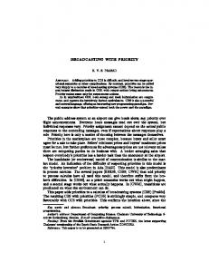
Constraint (i), leads to the following equation bounding the EDF scaling factor as a function of X: 2+ X (13) f 1( X ) = 1+ X Constraint (ii), leads to the following equation, also bounding the EDF scaling factor as a function of X: 2X + 2 f 2( X ) = (14) 2+ X Constraint (iii), again leads to an equation bounding the EDF scaling factor: f 3( X ) = 1 + X (15) As f 3( X ) ≥ f 2( X ) for all values of X, we may disregard f 3( X ) as f 2( X ) provides a tighter bound. Figure 4 illustrates the three functions bounding the EDF scaling factor for two tasks. Equation (13) is a continuous non-increasing function of X with a maximum value of f1(0) = 2. Equation (14) is a continuous non-decreasing function of X with a minimum value of f2(0) =1. Hence, the intersection of these two functions determines an upper bound on the maximum EDF scaling factor f. We have: 2 + X 2X + 2 = 1+ X 2+ X 2 (2 + X ) = (2 X + 2)(1 + X )

4. Processor speedup factor for constraineddeadline tasksets In this section, we derive the processor speedup factor for constrained-deadline tasksets under fixed priority pre-emptive scheduling. We do this first for tasksets of cardinality two and then for the general case of cardinality n. In each case, the basic approach we use is as follows: o First, we derive an upper bound on the maximum EDF scaling factor of the appropriate speedup-optimal taskset (defined in either Theorem 1 or Theorem 2), assuming any arbitrary value for the execution time X, of the lowest priority task. As part of this derivation, we determine the value of X that results in this upper bound. o Second, we prove that the maximum EDF scaling factor is in fact equal to the upper bound. We do this by showing that the speedupoptimal taskset, characterised by the previously obtained value of X, is schedulable according to EDF when all task execution times are scaled by the upper bound. This shows that the bound is tight. o Finally, the processor speedup factor for fixed priority pre-emptive scheduling is equal to the maximum EDF scaling factor (for any value of X) for the speedup-optimal taskset. So the processor speedup factor is equal to our tight upper bound.

X 2 + 4X + 4 = 2X 2 + 4X + 2 X2 =2

X = 2 f 2( 2 ) =

Speedup factor f

Theorem 3: For a constrained-deadline taskset of cardinality two, the processor speedup factor for fixed priority pre-emptive scheduling is 2 ≈ 1.414214 . Proof: We prove the theorem by determining the maximum EDF scaling factor for the taskset V described in Theorem 1, for any value of X. Three constraints on the EDF scheduling of the taskset described in Theorem 1, after it is scaled by a factor f are: Task τ 2 with execution time fX must (i) complete by its deadline at 2+X (subject to interference of f from task τ 1 ). The second invocation of task τ 1 must (ii) complete by its deadline at 2X+2. The total utilisation of task τ 1 must be less (iii) than or equal to 1 (The utilisation of task τ 2 is effectively zero as it has an infinite period).

2 2+2 2+ 2

2.5 2.4 2.3 2.2 2.1 2 1.9 1.8 1.7 1.6 1.5 1.4 1.3 1.2 1.1 1

=

2 (2 2 + 2) 2 2 +2

= 2

(16)

f1(X) f2(X) f3(X)

0

0.2

0.4

0.6

0.8

1

1.2

1.4

1.6

1.8

X

Figure 4: Constraints on the speedup factor for two tasks

To show that the maximum EDF scaling factor is equal to this upper bound, we must show that the taskset is schedulable, with scaled parameters, under EDF.

12

to τ n −1 described in Theorem 2, is given by: ⎛ 1 n−1 ⎞ 1 ⎟⎟ (21) U V = lim ⎜⎜ ∑ n−1→∞ ( n − 1) i =1 (1 + X + (i − 1) /( n − 1)) ⎠ ⎝ Substituting k = n-1 gives: ⎛1 k ⎞ 1 ⎟⎟ (22) U V = lim⎜⎜ ∑ k →∞ k + + − ( 1 X ( i 1 ) / k ) ⎝ i =1 ⎠ Equation (22) is recognisable as the Riemann sum7 of the function y =1/z over the partition [(1+X), (1+X)+1]. The start of each of the k intervals in the Riemann sum is at 1 + X + (i − 1) / k (for i = 1 to k), and the width of each interval is 1/k. The limit as k → ∞ of the Riemann sum is simply the integral over the partition so:

The scaled taskset parameters are as follows: C1 = 2 , D1 = 1 + 2 , T1 = 1 + 2 C 2 = 2 , D2 = 2 + 2 , T2 = ∞ The taskset is schedulable provided that ∀t h(t ) / t ≤ 1 (See Equation (2)). From Equation (2), we note that the maximum value of h(t ) / t occurs at the deadline of some invocation of a task. It is therefore sufficient to check that h(t ) / t ≤ 1 at the deadlines of all task invocations. For task τ 2 , there is only one deadline to consider, D2 = 2 + 2 , and: h(2 + 2 ) C 2 + C1 2 + 2 = = =1 (17) 2+ 2 2+ 2 2+ 2 For task τ 1 , there are deadlines to consider at times t = kD1 = k (1 + 2 ) , where k is a positive integer. For k = 1 , we have: C1 h(1 + 2 ) 2 (18) = = 1 , which is outside the permitted range of values for ε . Hence the maximum / minimum values of y (ε ) must occur for the maximum and minimum permitted values of ε . We now show that the range of values that ε can take is constrained by the fact that ⎣(k + 1) / Ω⎦ = ⎣k / Ω⎦ + 1 . Assuming that ε ≥ 2 − (1 / Ω) , then: k ⎢k ⎥ 1 ⎢k ⎥ (52) = +ε ≥ ⎢ ⎥ +2− Ω ⎢⎣ Ω ⎥⎦ Ω Ω ⎣ ⎦ and so k +1 ⎢ k ⎥ (53) ≥⎢ ⎥+2 Ω ⎣Ω⎦ which implies that ⎣(k + 1) / Ω ⎦ = ⎣k / Ω ⎦ + 2 . This contradicts the assumption that ⎣(k + 1) / Ω ⎦ = ⎣k / Ω ⎦ + 1 , and so ε is constrained (for this, Case 1) to be in the range 0 ≤ ε < 2 − (1 / Ω) . We now evaluate y (ε ) for the minimum and maximum possible values of ε . For ε = 0 , we have: (54) y (0) = k (1 / Ω − 1 − Ω) + 1 − 2Ω So y (0) ≥ 0 provided that: 2Ω − 1 (55) ≈ 0.684876 k≥ 1 / Ω − (1 + Ω) Hence ∀k ≥ 2 , y (0) ≥ 0 . For ε = 2 − (1 / Ω) , from Equation (49), we have: k 1⎞ ⎛ y (2 − (1 / Ω) ) = ⎜ 2Ω − 1 − 2k + + 2Ωk − k − 2 + ⎟ Ω Ω⎠ ⎝

(43)

Note that Equation (43) is only valid for k ≥ 2 , as for k = 1 , k + 1 > ⎣k / Ω ⎦ . As 1/z is a positive decreasing function, the summation term in Equation (43) is bounded by the following integral, (given that ⎣k / Ω ⎦ ≤ k / Ω ). k /Ω 1 ⎣k / Ω ⎦ 1 1 1 1 ⎛ ( k / Ω) ⎞ 1 ⎛ 1 ⎞ dz = ln⎜ ≤ ⎟ = ln⎜ ⎟ = 1 ∑ Ω j = k +1 j Ω j∫= k z Ω ⎝ k ⎠ Ω ⎝Ω⎠ As k → ∞ , ⎣k / Ω ⎦ → k / Ω hence we have: k →∞ 1 2 1 1 + − − +1 = 1 H (k ) = Ω k kΩ Ω □

(44) (45)

Lemma 12: ∀k ≥ 6 , H (k ) is a monotonic nondecreasing function, with H (k + 1) ≥ H (k ) . Proof: As 1 / Ω ≈ 1.76322 , there are two distinct cases to consider: Case 1: ⎣(k + 1) / Ω ⎦ = ⎣k / Ω ⎦ + 1 Case 2: ⎣(k + 1) / Ω ⎦ = ⎣k / Ω ⎦ + 2 Case 1: ⎣(k + 1) / Ω ⎦ = ⎣k / Ω ⎦ + 1 : From Equation (43) we have: k / Ω⎦ + 1 2 1 H (k + 1) − H (k ) = − −⎣ (k + 1) (k + 1)Ω (k + 1) +

k / Ω⎦ 1 ⎣k / Ω ⎦ 1 1 ⎣k / Ω ⎦+1 1 2 1 − + +⎣ − ∑ ∑ Ω j =k + 2 j k kΩ k Ω j =k +1 j

k / Ω⎦ − k 2 1 + +⎣ k (k + 1) k (k + 1)Ω k (k + 1) 1 1 + − Ω( ⎣k / Ω⎦ + 1) Ω(k + 1) (46) As we are interested only in showing that H (k + 1) − H (k ) ≥ 0 , we are free to multiply the expression in Equation (46) by any positive quantity. Multiplying by Ωk (k + 1)(⎣k / Ω ⎦ + 1) gives: ( ⎣k / Ω ⎦ + 1)(1 − 2Ω − k (1 + Ω) + Ω ⎣k / Ω⎦) + k (k + 1) (47) Substituting ⎣k / Ω ⎦ = (k / Ω) − ε , where ε is a value in the range 0 ≤ ε < 1 , gives: =−

2

1⎞ ⎛k ⎛ ⎞ + Ω⎜ 2 − ⎟ + ⎜ − k − Ωk + 1 − 2Ω ⎟ Ω⎠ ⎝Ω ⎝ ⎠ Simplifying:

16

(56)

⎛k ⎞ ⎛k ⎞ + k (k + 1)⎜ − ε + 1⎟ + k (k + 1)⎜ − ε + 2 ⎟ (61) ⎝Ω ⎠ ⎝Ω ⎠ Expanding we have: k 2 2k 2 2k 3 εk 2 2εk − − − − + 4εk + 4εk 2 + 2ε 2 k Ω Ω Ω Ω Ω2 3k + − 6k − 6k 2 − 3εk − 3ε + 6Ωε + 6Ωεk + 3Ωε 2 Ω + ε 2 − 2Ωε 2 − 2Ωε 2 k − Ωε 3 + 2 − 4Ω − 4Ωk − 2Ωε 2 k 3 2k 2 + + − 2εk 2 − 2εk + 3k 2 + 3k Ω Ω (62) For ease of reference, we refer to the expression in Equation (62) as the function y (ε ) . Simplifying and rearranging, we have: y (ε ) = (− Ω )ε 3

2

1⎞ 1⎞ ⎛ ⎛2 ⎞ ⎛ y (2 − (1 / Ω) ) = Ω⎜ 2 − ⎟ + k ⎜ − 4 + Ω ⎟ − ⎜ 2 − ⎟ Ω Ω Ω ⎝ ⎠ ⎝ ⎠ ⎝ ⎠ (57) So y (2 − (1 / Ω) ) ≥ 0 provided that: 2

1⎞ 1⎞ ⎛ ⎛ ⎜ 2 − ⎟ − Ω⎜ 2 − ⎟ Ω⎠ Ω⎠ ⎝ ⎝ k≥ ≈ 2.190228 ⎛2 ⎞ ⎜ − 4 + Ω⎟ ⎝Ω ⎠ Hence ∀k ≥ 3 , y (2 − (1 / Ω) ) ≥ 0 .

(58)

To summarise, (i) In this case, the range of potential values for ε is limited to 0 ≤ ε < 2 − (1 / Ω) ≈ 0.236778 . (ii) Equation (51) shows that provided k ≥ 2 , y (ε ) has no turning points in the range 0 ≤ ε < 1 , and so the maximum and minimum values of y (ε ) must occur for the maximum and minimum permitted values of ε . (iii) Equations (55) and (58) show that for k ≥ 3 , the maximum and minimum values of y (ε ) are both positive. We conclude that for k ≥ 3 , y (ε ) is always positive and hence for k ≥3 and ⎣(k + 1) / Ω ⎦ = ⎣k / Ω⎦ + 1 , H (k + 1) ≥ H (k ) .

+ (2k + Ω + 1 − 2Ωk )ε 2 ⎛ k 2 2k ⎞ + ⎜⎜ − − − k + 2k 2 − 3 + 4Ω + 6Ωk ⎟⎟ε Ω Ω ⎝ ⎠ +

(63) To find the minimum / maximum value of y (ε ) for any possible value of ε , we differentiate with respect to ε: dy = −3Ωε 2 + 2(2k + Ω + 1 − 2Ωk )ε dε ⎛ k 2 2k ⎞ + ⎜⎜ − − − k + 2k 2 − 3 + 4Ω + 6Ωk ⎟⎟ Ω Ω ⎝ ⎠

Case 2: ⎣(k + 1) / Ω ⎦ = ⎣k / Ω ⎦ + 2 : From Equation (43) we have: k / Ω⎦ + 2 2 1 H (k + 1) − H (k ) = − −⎣ (k + 1) (k + 1)Ω (k + 1) +

k 2 3k + − 3k − 3k 2 + 2 − 4Ω − 4Ωk Ω2 Ω

k /Ω 1 ⎣k / Ω ⎦+ 2 1 2 1 ⎣k / Ω⎦ − 1 ⎣ ⎦ 1 − + + ∑ ∑ Ω j =k + 2 j k kΩ k Ω j =k +1 j

(64) The turning points (minimum / maximum values) of y (ε ) occur when dy / dε = 0 , i.e. for the values of ε given by the solutions to a quadratic equation, formed from the expression in Equation (64). The solutions to a quadratic equation of the form aε 2 + bε + c = 0 are given by:

k / Ω ⎦ − 2k 2 1 + +⎣ k (k + 1) k (k + 1)Ω k (k + 1) 1 1 1 + + − Ω( ⎣k / Ω⎦ + 2) Ω( ⎣k / Ω ⎦ + 1) Ω(k + 1) (59) As we are interested only in showing that H (k + 1) − H (k ) ≥ 0 , we are free to multiply the expression in Equation (59) by any positive quantity. Multiplying by Ωk (k + 1)( ⎣k / Ω ⎦ + 1)(⎣k / Ω ⎦ + 2) gives: ( ⎣k / Ω ⎦ + 2)( ⎣k / Ω ⎦ + 1)(1 − 2Ω − k (1 + 2Ω) + Ω ⎣k / Ω ⎦) =−

− b ± b 2 − 4ac (65) 2a We are interested in the case where the turning points of y (ε ) occur outside of the permitted range of values for ε ( 0 ≤ ε < 1 ). From Equation (65), we can see that this is the case provided that (−b / 2a ) > 1 / 2 and −4ac ≥ 0 , as the two solutions are then less than zero and greater than one respectively. Now as − b 4k (1 − Ω) + 2(1 + Ω ) (66) = 2a 6Ω (−b / 2a ) > 1 / 2 provided that: 3Ω − 2(1 + Ω ) (67) k> ≈ −0.827557 4(1 − Ω)

ε=

+ k (k + 1)( ⎣k / Ω ⎦ + 1) + k (k + 1)( ⎣k / Ω ⎦ + 2) (60) Substituting ⎣k / Ω ⎦ = (k / Ω) − ε , where ε is a value in the range 0 ≤ ε < 1 , gives: ⎛k ⎞⎛ k ⎞ ⎜ − ε + 2 ⎟⎜ − ε + 1⎟(1 − 2Ω − 2Ωk − Ωε ) ⎝Ω ⎠⎝ Ω ⎠

17

hence for k ≥ 6 H (k + 1) ≥ H (k ) .

Further, ⎛ k 2 2k ⎞ − 4ac = 12Ω⎜⎜ − − − k + 2k 2 − 3 + 4Ω + 6Ωk ⎟⎟ ⎝ Ω Ω ⎠ (68) So −4ac ≥ 0 provided that: 1⎞ 2 ⎛ 2⎞ ⎛ (69) ⎜ 2 − ⎟k + ⎜ 6Ω − 1 − ⎟k − 3 + 4Ω ≥ 0 Ω⎠ Ω⎠ ⎝ ⎝ Evaluating the coefficients in Equation (69), we have: 1.611439k 2 − 7.646811k − 4.977885 ≥ 0 (70) Solving for k, gives: k = 2.372665 ± 2.952733 (71) Therefore, ∀k ≥ 6 , the inequality in Equation (70) holds and the turning points of y (ε ) occur outside of the permitted range of values of ε . Thus ∀k ≥ 6 the maximum / minimum values of y (ε ) must occur for the maximum and minimum permitted values of ε . From Equation (63), for ε = 0 , we have: ⎛ 1 ⎞ ⎛3 ⎞ (72) y (0) = ⎜ 2 − 3 ⎟k 2 + ⎜ − 3 − 4Ω ⎟k + 2 − 4Ω ⎝Ω ⎠ ⎝Ω ⎠ Evaluating the coefficients in Equation (72), gives: 0.1089547 k 2 − 0.02109534k − 0.26857316 ≥ 0 (73) Hence, ∀k ≥ 2 , y (0) ≥ 0 . From Equation (63), for ε = 1 , we have: y (1) = −Ω + 2k + Ω + 1 − 2Ωk

and

⎣(k + 1) / Ω ⎦ = ⎣k / Ω ⎦ + 2 ,

Combining the results for Case 1 and Case 2, shows that ∀k ≥ 6 , H (k + 1) ≥ H (k ) □ Lemma 13: ∀k ≤ 6 , H (k ) ≤ 1 . Proof: Recall that H (k ) is defined by Equation (39) as the value of the processor load h(t ) / t at discrete points in time given by t = k (2 + X ) , for k = 1..∞ , where h(t ) is the processor demand bound function given by Equation (34).

First we consider the case where k = 1 . For k = 1 , we have: f (1 + X ) (77) =1 H (k ) = (2 + X ) Table 2 below gives the computed values of H (k ) , for k = 1..6 . Table 2

k 1 2 3 4 5 6

k 2 2k − − k + 2k 2 − 3 + 4Ω + 6Ωk Ω Ω k 2 3k + 2 + − 3k − 3k 2 + 2 − 4Ω − 4Ωk Ω Ω −

H(k) 1 0.969352362 0.968932165 0.970821141 0.976740571 0.980546791

□ Lemma 11 showed that as k → ∞ , H (k ) → 1 , Lemma 12 showed that ∀k ≥ 6 , H (k ) is a monotonic nondecreasing function of k, and Lemma 13 showed that ∀k ≤ 6 , H (k ) ≤ 1 . It follows that ∀k ≥ 1 H (k ) ≤ 1 . As the maximum points of the function h(t ) / t are given by the values of H (k ) , we conclude that: h(t ) (78) ∀t ≤1 t and hence that the taskset in Theorem 2, with the value of X defined by Equation (31), is schedulable under EDF with all execution times scaled by a factor of 1 / Ω . Given the constraints expressed in Equations (24) and (25), the maximum EDF scaling factor, for any value of X, is therefore 1 / Ω . For a constrained-deadline taskset of arbitrary cardinality, the processor speedup factor for fixed priority pre-emptive scheduling is equal to the maximum EDF scaling factor (for any value of X) for the speedupoptimal taskset described in Theorem 2 □

(74) Simplifying Equation (74) gives: 1 ⎛ 1 ⎞ ⎛1 ⎞ (75) y (1) = ⎜ 2 − − 1⎟k 2 + ⎜ − 2 ⎟k Ω Ω Ω ⎝ ⎠ ⎝ ⎠ Evaluating the coefficients in Equation (75), gives: y (1) = 0.34573192k 2 − 0.23677716k (76) Hence, ∀k ≥ 2 , y (1) ≥ 0 . (From Equation (76), y (1) is positive provided that k ≥ 1 ; however, our analysis is only valid for k ≥ 2 ). To summarise, (i) In this case, the range of potential values for ε is bounded by 0 ≤ ε < 1 . (ii) Equations (64) to (71) show that provided k ≥ 6 , y (ε ) has no turning points in the range 0 ≤ ε < 1 , and so the maximum and minimum values of y (ε ) must occur for the maximum and minimum values of ε . (iii) Equations (73) and (76) show that for k ≥ 2 , the values of y (0) and y (1) are both positive. We conclude that for k ≥ 6 , y (ε ) is always positive and

Corollary 6: The maximum EDF scaling factor and hence the processor speedup factor for a constrained-

18

deadline taskset of any cardinality is achieved for the speedup-optimal taskset described in Theorem 2, with an execution time for the lowest priority task of X = (2Ω − 1) /(1 − Ω) ≈ 0.312333 .

f ( X ) , against values of X. f(X)

1.25 1.225

5. Processor speedup factor for implicitdeadline tasksets

Speedup factor f

1.2

In this section, we extend the results of Sections 3 and 4 to implicit-deadline tasksets ( ∀i Di = Ti ). Before considering tasksets of arbitrary cardinality, we first present results for tasksets comprising just two tasks. The derivation of this result again provides the intuition for the general case.

1.175 1.15 f(X)

1.125 1.1 1.075 1.05 1.025

Theorem 5: For the class of tasksets with implicit deadlines and cardinality two, there is a speedup-optimal taskset V, which has the following parameters: Taskset V is identical to the taskset described in Theorem 1 with the exception that the period of task τ n , rather than being infinite, is equal to its deadline.

1 0

0.4 0.8 1.2

1.6

2

2.4 2.8 3.2 3.6

X

Figure 7: Speedup factor for 2 tasks with D=T

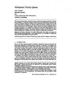
Equation (80), is a continuous function of X, with maximum / minimum values where the first derivative with respect to X is zero. df − X2 +2 = (81) dX ( X 2 + 2 X + 2) 2

Proof: As the class of implicit-deadline tasksets is a subset of the class of constrained-deadline tasksets, proof follows directly from the proof of Theorem 1, noting that Lemma 2 does not apply and instead we have the constraint that Tn = Dn □

Hence the maximum value occurs for X = 2 , resulting in a maximum EDF scaling factor of: 4+3 2 1 f ( 2) = = ≈ 1.207107 (82) 4 + 2 2 2( 2 − 1) For an implicit-deadline taskset of cardinality two, the processor speedup factor for fixed priority preemptive scheduling is equal to the maximum EDF scaling factor (for any value of X) for the speedupoptimal taskset described in Theorem 5 □

Theorem 6: For an implicit-deadline taskset of cardinality two, the processor speedup factor for fixed priority pre-emptive scheduling is 1 / 2( 2 − 1) ≈ 1.207107 . Proof: We prove the theorem by determining the maximum EDF scaling factor for the taskset V described in Theorem 5, for any value of X. As taskset V is an implicit-deadline taskset, a sufficient and necessary condition for schedulability under EDF, is that the total utilisation of the taskset must be less than or equal to 1, after the task execution times are scaled by a factor of f. The total utilisation of the tasks is given by: 2 1 X (79) ∑U i = 1 + X + 2 + X i =1 Therefore, assuming total utilisation U = 1, we have the following equation for the maximum EDF scaling factor as a function of X. 1 f (X ) = X ⎞ ⎛ 1 + ⎜ ⎟ 1 + X 2 + X⎠ ⎝

Corollary 7: As EDF is known to schedule any implicitdeadline taskset, provided that U ≤ 1 , Theorem 6 shows that fixed priority pre-emptive scheduling can schedule any implicit-deadline taskset of cardinality two, provided that U ≤ 2( 2 − 1) ≈ 0.828427 , in agreement with, and providing a diverse proof of, the result of Fineberg and Serlin (1967).

We note that this speedup-optimal taskset for the implicit-deadline case and cardinality two, is the one used as an illustrative example in Section 2.6. Theorem 7: For the class of implicit-deadline tasksets with arbitrary cardinality, there is a speedup-optimal taskset V, which has the following parameters: Taskset V is identical to the taskset described in Theorem 2 with the exception that the period of task τ n , rather than being infinite, is equal to its deadline.

(1 + X )(2 + X ) X 2 + 3X + 2 (80) = 2 (2 + X ) + (1 + X ) X X + 2X + 2 Figure 7 plots the maximum EDF scaling factor =

19

Proof: As the class of implicit-deadline tasksets is a subset of the class of constrained-deadline tasksets, proof follows directly from the proof of Theorem 2, noting that Lemma 2 does not apply and instead we have the constraint that Tn = Dn □

f(X) 1.5 1.45

Speedup factor f

1.4

Theorem 8: For an implicit-deadline taskset of arbitrary cardinality, the processor speedup factor for fixed priority pre-emptive scheduling is 1 / ln(2) ≈ 1.44270 . Proof: We prove the theorem by determining the maximum EDF scaling factor for the taskset V described in Theorem 7, for any value of X. As taskset V is an implicit-deadline taskset, a sufficient and necessary condition for schedulability under EDF, is that the total utilisation of the taskset must be less than or equal to 1, after the task execution times are scaled by a factor of f. From Lemma 10, the total utilisation of the tasks τ 1..τ n−1 is given by: n −1 ⎛2+ X ⎞ (83) ∑U i = ln⎜⎝ 1 + X ⎟⎠ i =1 Further, the utilisation of task τ n is: X (84) Un = 2+ X Therefore, assuming total utilisation U = 1, we have the following equation for the maximum EDF scaling factor as a function of X. 1 (85) f (X ) = ⎛ ⎛2+ X ⎞ X ⎞ ⎜⎜ ln⎜ ⎟ + ⎟ ⎟ ⎝ ⎝ 1+ X ⎠ 2 + X ⎠ Figure 8 plots the maximum EDF scaling factor, against values of X. Equation (85), is a continuous non-increasing function of X, with a maximum value f (0) = 1 / ln(2) . The maximum EDF scaling factor is therefore 1 / ln(2) ≈ 1.44270 , which occurs as the execution time X of the lowest priority task tends to zero. For an implicit-deadline taskset of arbitrary cardinality, the processor speedup factor for fixed priority pre-emptive scheduling is equal to the maximum EDF scaling factor (for any value of X) for the speedupoptimal taskset described in Theorem 7 □

f(X)

1.35 1.3 1.25 1.2 1.15 1.1 1.05 1 0

1

2

3

4

5

6

7

8

9

X

Figure 8: Speedup factor for n tasks with D=T Corollary 8: As EDF is known to schedule any implicitdeadline taskset, provided that U ≤ 1 , Theorem 7 shows that fixed priority pre-emptive scheduling can schedule any implicit-deadline taskset, provided that U ≤ ln(2) ≈ 0.693147 , in agreement with, and providing a diverse proof of, the well known result of Liu and Layland (1973).

6. Summary and Conclusions In this paper, we have examined the relative effectiveness of fixed priority pre-emptive scheduling for sporadic / periodic tasks with constrained deadlines ( Di ≤ Ti ). Our metric for measuring the effectiveness of this scheduling policy is a resource augmentation factor known as the processor speedup factor. The processor speedup factor is defined as the maximum amount by which the execution time of all tasks in a taskset that is only just schedulable under fixed priority pre-emptive scheduling can be scaled up and the taskset remain feasible (i.e. schedulable under an optimal algorithm such as EDF). An alternate and equivalent definition of the processor speedup factor is the maximum amount by which the processor needs to be speeded up so that any taskset that is feasible (i.e. schedulable by an optimal algorithm such as EDF) can be guaranteed to be schedulable under fixed priority pre-emptive scheduling. The major contributions of this paper are as follows: o Deriving the structure and parameters of a speedup-optimal taskset that provides a tight bound on the processor speedup factor for constrained-deadline tasksets. o Proving that the processor speedup factor for constrained-deadline tasksets of cardinality two, is 2 ≈ 1.414214 . o Proving that the processor speedup factor for constrained-deadline tasksets of arbitrary

20

cardinality, is 1 / Ω ≈ 1.76323 . Deriving, in Appendix A, an upper bound on the processor speedup factor for small n which improves upon the general result for constrained-deadline tasksets of arbitrary cardinality. o Proving that the processor speedup factor for implicit-deadline tasksets of cardinality two is 1 / 2( 2 − 1) ≈ 1.207107 . A result that provides a diverse proof of one of the earliest published results on fixed priority schedulability analysis, the sufficient schedulability test U ≤ 2( 2 − 1) for two tasks by Fineberg and Serlin (1967). o Proving that the processor speedup factor for implicit-deadline tasksets of arbitrary cardinality is 1 / ln(2) ≈ 1.44270 . A result that is in agreement with, and provides a diverse proof of, the well known sufficient schedulability test U ≤ ln(2) of Liu and Layland (1973). The seminal work of Liu and Layland (1973) characterises the maximum performance penalty incurred when an implicit-deadline taskset is scheduled using rate-monotonic, fixed priority pre-emptive scheduling instead of an optimal algorithm such as EDF. The research in this paper provides an analogous characterisation of the maximum performance penalty incurred when constrained-deadline tasksets are scheduled using deadline-monotonic, fixed priority preemptive scheduling instead of an optimal algorithm such as EDF. Table 3 summarises the extent of these performance penalties. Table 3

6.1. Future work

o

Optimal (e.g. EDF) Implicitdeadline Constrained -deadline

U ≤1 LOAD ≤ 1

Fixed Priority U ≤ ln(2) ≈ 0.693147 LOAD ≤ Ω ≈ 0.567143

In future, we intend to investigate the sub-optimality of fixed priority pre-emptive scheduling with respect to arbitrary-deadline tasksets, where task deadlines may be less than, equal to, or greater than their periods. To the best of our knowledge, no research has yet been done to characterise the average-case suboptimality of fixed priority pre-emptive scheduling for constrained-deadline tasksets. This is also an interesting area for future research.

6.2. Acknowledgements This work was funded in part by the EU Frescor, eMuCo and Jeopard projects.

Appendix A: Processor speedup factor for constrained-deadline tasksets with cardinality n In this appendix, we provide an upper bound on the processor speedup factor for fixed priority pre-emptive scheduling of constrained-deadline tasksets comprising a small number of tasks. Theorem A.1: For the class of tasksets with constrained deadlines and cardinality n, there is a speedup-optimal taskset V, with α V = 1, which has the following parameters: ∀i ≠ n Di = Ti = ∑ C j + C n + ∑ C j ∀j∈hp ( n )

∀j∈hp (i )

Dn = 1 , Tn = ∞ (A.1) Note that in Theorem A.1, the deadline of task τ n has been normalised to 1 and the other task periods and deadlines adjusted accordingly. Further, the task execution times are free variables, subject to the constraint: 2 ∑ C j + Cn = 1 (A.2)

Speedup factor 1 / ln(2) ≈ 1.44270 1/ Ω ≈ 1.76323

∀j∈hp ( n )

Proof: Proof follows directly from Lemmas 1 to 8, specifically: o τ n must be a constraining task, with the longest deadline and the lowest priority (Lemma 1). o τ n must have an infinite period (Lemma 2). o t = Dn must be the start of an idle period (Lemma 3). o ∀i ≠ n Ti < Dn (Lemma 4) o ∀i ≠ n Di = Ti (Lemma 5). o ∀i ≠ n Ti > Dn / 2 (Lemma 6). o Following a critical instant, τ n must execute continuously from when it first starts execution until it completes (Lemma 7). o The task parameters must comply with the following equation (Lemma 8):

Note that although in this paper, we have made numerous references to EDF as an example of an optimal pre-emptive uniprocessor scheduling algorithm, and made use of results about EDF in our proofs, our results are valid with respect to any optimal pre-emptive uniprocessor scheduling algorithm, for example Least Laxity First (Mok, 1983). This is because all such optimal algorithms can by definition schedule exactly the same set of tasksets: all those that are feasible. In conclusion, this paper provides for the first time, a tight bound on the sub-optimality of fixed priority preemptive scheduling for uniprocessor systems with constrained-deadlines.

21

∀i ≠ n Di = Ti = ∑ C j + ∀j

∑C j

other task parameters. Note that taskset V ′ is unschedulable according to fixed priority pre-emptive scheduling as τ n misses its deadline. From Equation (A.2) which holds for taskset V, for taskset V ′ we have: 2 ∑ C j + Cn > 1 (A.10)

∀j∈hp (i )

□ Lemma A.1: The following inequality holds for any implicit-deadline taskset W, with cardinality n > 2 that is not schedulable according to fixed priority preemptive scheduling: ⎞ ⎛ 2 (A.3) ∑U j > (n − 1)⎜⎜ (n−1) 1 + U − 1⎟⎟ n ∀j∈hp ( n ) ⎠ ⎝

∀j∈hp ( n )

We now consider the total utilisation U of taskset V ′ . Observe that if we set the period of task τ n equal to its deadline ( Tn = Dn = 1 ), then this transforms V ′ into an implicit deadline taskset W, which is unschedulable according to fixed priority pre-emptive scheduling, as taskset V ′ is already unschedulable with τ n = ∞ . From Lemma A.1, as Tn = 1 for the implicitdeadline taskset W, we have: ⎞ ⎛ 2 (A.11) ∑U j > (n − 1)⎜⎜ (n−1) 1 + C − 1⎟⎟ n ∀j∈hp ( n ) ⎠ ⎝ As Tn = ∞ in taskset V ′ , U n = 0 , and so the LHS of Equation (A.11) corresponds to the total utilisation U of taskset V ′ . Hence we have: ⎞ ⎛ 2 (A.12) U > (n − 1)⎜ (n−1) − 1⎟ ⎟ ⎜ 1 + Cn ⎠ ⎝ Now consider taskset V ′ scheduled according to EDF. Taskset V ′ is schedulable according to EDF if and only if: ⎛ h(t ) ⎞ max⎜ (A.13) ⎟ ≤1 ∀t ⎝ t ⎠ where h(t ) is the processor demand bound function defined by Equation (2). Now, ⎛ h(t ) ⎞ ⎛ h(1) h(∞) ⎞ max⎜ , ⎟ ≥ max⎜ ⎟ = max(h(1),U ) ∀t ⎝ t ⎠ ∞ ⎠ ⎝ 1 (A.14) From Equation (2): h(1) = ∑ C j + C n (A.15)

Proof: As taskset W is unschedulable, it cannot be schedulable according the Hyperbolic bound (Bini et al., 2003). Hence: (A.4) ∏ 1+U j > 2

(

)

∀j

Consider the arithmetic and geometric means of the series of values (1 + U j ) , ∀j ∈ hp (n) . By the inequality of arithmetic and geometric means, we have: ⎛1+U j ⎞ (A.5) ∑ ⎜⎜ n − 1 ⎟⎟ ≥(n−1) ∏ 1 + U j ∀j∈hp ( n ) ⎝ ∀j∈hp ( n ) ⎠ Substituting for the Hyperbolic bound divided by 1 + U n , into Equation (A.5) gives: ⎛1+U j ⎞ 2 (A.6) ∑ ⎜⎜ n − 1 ⎟⎟ > (n−1) 1 + U n ∀j∈hp ( n ) ⎝ ⎠

(

)

As: ⎞ − 1⎟ ⎟ ⎝ ∀j∈hp ( n) (n − 1) ⎠ ⎛

1+U j

⎛

2

∑U j = (n − 1)⎜⎜ ∑

∀j∈hp ( n )

(A.7)

it follows that:

∑U j > (n − 1)⎜⎜ (n−1) 1 + U

∀j∈hp ( n )

⎝

n

⎞ − 1⎟ ⎟ ⎠

(A.8)

□

∀j∈hp ( n )

Substituting for the summation term from Equation (A.10) gives: 1 + Cn h(1) > (A.16) 2 Substituting the total utilisation U from Equation (A.12) and the processor demand bound function h(1) from Equation (A.16) into Equation (A.14) gives: ⎛⎛1+ C ⎞ ⎛ ⎞⎞ 2 ⎛ h(t ) ⎞ n max⎜ − 1⎟ ⎟ ⎟, (n − 1)⎜⎜ ( n−1) ⎟ > max⎜ ⎜ ⎟⎟ ⎜⎝ 2 ⎠ ∀t ⎝ t ⎠ 1 + Cn ⎝ ⎠⎠ ⎝ (A.17) For any given value of n ≥ 2 , the left hand term within the max expression, is a monotonically increasing function of C n , whilst the right hand term is a monotonically decreasing function of C n . Hence the minimum value L(n) , of the max expression is achieved

Theorem A.2: For a constrained-deadline taskset, of cardinality n ≥ 2 , an upper bound on the processor speedup factor for fixed priority pre-emptive scheduling is given by f UB (n) , where f UB (n) is defined as follows: f UB (n) = 1 / L(n) Where L(n) forms the solution to the following equality, where C n may take any non-negative real value: ⎞ ⎛ 2 ⎛ 1 + Cn ⎞ (A.9) L( n) = ⎜ − 1⎟ ⎟ = (n − 1)⎜⎜ (n−1) ⎟ 1 + Cn ⎝ 2 ⎠ ⎠ ⎝ Proof: Let taskset V ′ be formed from taskset V in Theorem A.1 by an infinitesimal increase in the execution time of task τ n , with no changes to any of the

22

when these two terms are equal. ⎞ ⎛ 2 ⎛ 1 + Cn ⎞ (A.18) L( n) = ⎜ − 1⎟ ⎟ = (n − 1)⎜⎜ ( n−1) ⎟ 1 + Cn ⎝ 2 ⎠ ⎠ ⎝ Let us assume that taskset V ′ , which we know is unschedulable according to fixed priority pre-emptive scheduling, was obtained from a taskset S ′ by applying a processor speedup factor f ≥ f UB (n) = 1 / L(n) , such that the execution times of the tasks in taskset S ′ are f times those of the corresponding tasks in taskset V ′ . Equation (A.19) shows that taskset S ′ cannot be schedulable according to EDF, as: f ⎛ h(t ) ⎞ (A.19) max⎜ ≥1 ⎟> ∀t ⎝ t ⎠ L( n) Hence using a processor speedup factor f ≥ f UB (n) , it is not possible to obtain a taskset V ′ that is unschedulable according to fixed priority pre-emptive scheduling, from a taskset S ′ that is schedulable according to EDF. Recall that taskset V ′ is related to the speedupoptimal taskset V of Theorem A.1 via an infinitesimal increase in the execution time of task τ n . We conclude that there can be no tasksets, that are schedulable according to EDF that are unschedulable according to fixed priorities, when a processor speedup factor of f ≥ f UB (n) is applied. f UB (n) is therefore an upper bound on the processor speedup factor for constraineddeadline tasksets of cardinality n, which is sufficient to ensure that any such taskset that is schedulable according to an optimal scheduling policy (e.g. EDF) remains schedulable according to fixed priority preemptive scheduling □

Table 5

n 2 4 8 16 32 64 128 256 ∞

Table 4 L(n) 0.618034 0.594313 0.585670 0.581198 0.578464 0.576621 0.575294 0.574293

f UB ( n) 1.619 1.683 1.708 1.721 1.729 1.735 1.739 1.742

f UB ( n) 1.619 1.708 1.739 1.752 1.758 1.761 1.762 1.763 1/ Ω

f LB (n) 1.414 1.656 1.723 1.749 1.757 1.759 1.761 1.762 1/ Ω

To complement the upper bounds given by Theorem A.2, Table 4 and Table 5 also give lower bounds f LB (n) on the processor speedup factor. These lower bounds are necessary to schedule tasksets whose parameters comply with Theorem A.1. The lower bounds were found by searching for tasksets of the desired cardinality that comply with Theorem A.1 and remain schedulable according to EDF when their execution times are scaled up by the maximum possible scaling factor f. The search for these tasksets, and hence the lower bounds, involved iterating over: (i) A range of possible values for the EDF scaling factor f from 1.4 to 1.77 in steps of 0.001. (ii) A range of possible values for C n as a proportion of the total execution time of the higher priority tasks τ 1 to τ n −1 , from 0.001 to 2.0. (iii) (a) Arithmetic progressions in the values of C1 to C n−1 , with a range of increments from 0.0 to 1.0 times C1 in steps of 0.001 times C1 . (b) Geometric progressions in the values of C1 to C n−1 , with multiplying factors from 1.0 to 1.5 in steps of 0.001. The lower bounds in Table 4 and Table 5 are effectively rounded down to ensure necessity. Note that the types of taskset used to determine these lower bounds are only known to be speedup-optimal for n = 2 and n = ∞ . Figure 9 plots the upper and lower bounds for small values of n, from Table 4. The difference between the upper and lower bounds is less than 1% for tasksets of cardinality of 7 or more.

We observe that f UB (n) is an upper bound, as opposed to an exact value, due to the fact that the Hyperbolic bound used in its derivation is a sufficient but not necessary schedulability test, and also due to the inequality in Equation (A.14). Table 4 and Table 5 give the values of L(n) and f UB (n) as a function of n, computed by numerical approximation. Note the values of f UB (n) have been rounded up, to ensure sufficiency.

n 2 3 4 5 6 7 8 9

L(n) 0.618034 0.585670 0.575294 0.570987 0.569012 0.568065 0.567601 0.567371 Ω

f LB (n) 1.414 1.587 1.656 1.684 1.704 1.718 1.723 1.730

23

1

1.8 1.75 1.708

1.729

1.683

1.7 Processor Speedup Factor

1.721

1.704 1.65

1.735

1.739

1.742

1.718

1.723

1.730

1.656

Lower Bound 1.587

1.55 1.5 1.45 1.4

1.414

1.35 2

3

4

5

6

7

8

9

Number of Tasks

Figure 9: Upper and lower bounds on the Speedup factor for n tasks with D≤T

Similarly, Figure 10 plots the upper and lower bounds from Table 5, for values of n from 2 to 256. The difference between the upper and lower bounds is less than 0.1% for tasksets of cardinality of 32 or more. 1.8 1.739

1.75 1.708 Processor Speedup Factor

1.7 1.65

1.752 1.749

1.758

1.761

1.762

1.763

1.757

1.759

1.761

1.762

1.723 1.619

1.656 Upper Bound Lower Bound

1.6

1.5 1.45

1.414

1.35 2

4

8

16

32

64

128

(A.20)

In summary, to guarantee schedulability of any constrained-deadline taskset of cardinality n under fixed priority pre-emptive scheduling it is sufficient to use a speedup factor equal to the upper bound values f LB (n) given in Table 4 and Table 5. For small n, this represents an improvement over using the exact value for arbitrary n ( 1 / Ω ≈ 1.763223 ).

1.55

1.4

⎞ ⎟

⎛ 2 ⎞ ⎛ 1 U ⎞ ⎟⎟ ⎟⎟ > ln⎜⎜1 + ln⎜⎜ (A.21) ⎝ (n − 1) ⎠ (n − 1) ⎝ 1 + C n ⎠ From the Maclaurin expansion of ln(1 + x) , as x → 0 , ln(1 + x) → x , hence as n → ∞ , we have: ⎛ 2 ⎞ ⎟⎟ (A.22) U > ln⎜⎜ ⎝ 1 + Cn ⎠ We observe that Equation (A.22) holds for any value of n ≥ 2 and 0 < U ≤ 1 , as x > ln(1 + x ) for 0 < x ≤ 1 . Substituting for U from Equation (A.22) into Equation (A.14) yields the following, in place of Equation (A.17): ⎛ ⎛ 1 + Cn ⎞ ⎛ 2 ⎞ ⎞ ⎛ h(t ) ⎞ ⎟⎟ ⎟ (A.23) max⎜ ⎟, ln⎜⎜ ⎟ > max⎜⎜ ⎜ ⎟ ∀t ⎝ t ⎠ 2 1 C + ⎝ ⎠ n ⎠⎠ ⎝ ⎝ As in Equation (A.17), the left hand term within the max expression of Equation (A.23), is a monotonically increasing function of C n , whilst the right hand term is a monotonically decreasing function of C n . Hence the minimum value L(∞) , of the max expression is achieved when these two terms are equal. ⎛ 2 ⎞ ⎛ 1 + Cn ⎞ ⎟⎟ L (∞ ) = ⎜ (A.24) ⎟ = ln⎜⎜ 2 ⎝ ⎠ ⎝ 1 + Cn ⎠ This occurs for a value of L(∞) = Ω . (Where Ω is the mathematical constant defined by ln(1 / Ω) = Ω . Hence, Ω ≈ 0.567143 ). Finally, f UB (∞) = 1 / L(∞ ) = 1 / Ω □

Upper Bound

1.6

2

Hence:

1.684 1.619

⎛ ⎜

ln U 2 ( n −1) ⎜⎝ 1+Cn ⎟⎠ > ( n−1) =e 1+ (n − 1) 1 + Cn

Appendix B:

256

Number of tasks

In this appendix, we prove that the two alternate definitions for the processor speedup factor given in Section 2.5 are equivalent.

Figure 10: Upper and lower bounds on the Speedup factor for n tasks with D≤T

Theorem B.1: Definition 2 is equivalent to Definition 1 with fixed priority pre-emptive scheduling as scheduling algorithm A.

Theorem A.3: For a constrained-deadline taskset, of cardinality n, the upper bound f UB (n) on the processor speedup factor for fixed priority pre-emptive scheduling tends to 1 / Ω as n tends to infinity.

According to Definition 1, let f (Ψ ) be the minimum speedup factor required to make a feasible taskset Ψ schedulable according to fixed priority pre-emptive scheduling.

Proof: Follows the same logic as the proof of Theorem A.2. From Equation (A.12), we have:

24

algorithm (e.g. EDF). This is Definition 2 □

Lemma B.1: Let Z be the set of all feasible tasksets. Note, by Definition 1, Z contains at least one taskset that requires the (maximum) processor speedup-factor f A to be schedulable under fixed priority pre-emptive scheduling. Let Y ⊆ Z be the set of all feasible tasksets that will become infeasible when their execution times are scaled by any factor >1. The set Y contains at least one taskset that requires the (maximum) processor speedup-factor f A .

References Audsley N.C., Burns A., Richardson M., Wellings A.J. (1993) “Applying new Scheduling Theory to Static Priority Preemptive Scheduling”. Software Engineering Journal, 8(5) pp. 284-292. Baruah S., Burns A. (2006) “Sustainable Scheduling Analysis”. In Proceedings of the IEEE Real-Time Systems Symposium, pp. 159-168. Baruah S., Burns A. (2008) “Quantifying the sub-optimality of uniprocessor fixed priority scheduling.” In Proceedings of the IEEE International conference on Real-Time and Network Systems pp. 89-95. Baruah S.K., Mok A.K., Rosier L.E. (1990b) “Preemptively Scheduling Hard-Real-Time Sporadic Tasks on One Processor”. In Proceedings of the IEEE Real-Time System Symposium, pp.182-190. Baruah S.K., Rosier L.E., Howell R.R. (1990a) “Algorithms and Complexity Concerning the Preemptive Scheduling of Periodic Real-Time Tasks on one Processor”. Real-Time Systems, 2(4):301-324. E. Bini, G.C. Buttazzo (2005), Measuring the Performance of Schedulability Tests, Real-Time Systems 30 (1-2), pp. 129154. Bini E., Buttazzo G.C., Buttazzo G.M. (2003) “Rate Monotonic Scheduling: The Hyperbolic Bound”. IEEE Transactions on Computers, 52(7):933–942. Dertouzos M.L. (1974) “Control Robotics: The Procedural Control of Physical Processes”. In Proceedings of the IFIP congress, pp.807-813. Fineberg M.S., Serlin O., “Multiprogramming for hybrid computation”, In proceedings AFIPS Fall Joint Computing Conference, pp 1-13, 1967 Joseph M., Pandya P.K. (1986) “Finding Response Times in a Real-time System”. The Computer Journal, 29(5):390–395.

Proof: We assume (for contradiction) that there is a taskset Ψ that is a member of Z, but not a member of Y ( Ψ ∈ Z ∩ Y c ) that has a speedup factor f (Ψ ) strictly greater than that of any taskset which is only just feasible, (and therefore a member of Y). We note that Ψ can have its execution times scaled by a factor >1 and remain feasible, otherwise it would be a member of Y. We now construct a new taskset Φ from taskset Ψ by scaling all of the execution times of the tasks in Ψ by a factor >1, such that the resulting taskset is only just feasible, hence Φ ∈ Y . From Equation (1), increasing the execution time of tasks cannot make a taskset schedulable under fixed priority pre-emptive scheduling. Hence the speedup factor required by taskset Φ must be at least as large as that required by taskset Ψ (i.e. f (Φ ) ≥ f (Ψ ) ) which contradicts the original assumption. Hence there are no tasksets in Z ∩ Y c that require a speedup factor exceeding the maximum speedup factor required by any taskset in Y. As there was, by definition, at least one taskset in Z that required the maximum processor speedup factor, then there must also be at least one such taskset in Y □

Kalyanasundaram B., Pruhs K. (1995), “Speed is as powerful as clairvoyance”. In Proceedings of the 36th Symposium on Foundations of Computer Science, pp. 214--221.

Proof (of Theorem B.1): Lemma B.1 shows that there is at least one taskset that is only just schedulable according to an optimal algorithm such as EDF and requires the maximum processor speedup factor, according to Definition 1 to be schedulable under fixed priority pre-emptive scheduling. Let Φ be such a taskset. Increasing processor speed by a factor f is equivalent to reducing task execution times by the same factor. By definition of the speedup factor f (Θ) , reducing the execution times of the tasks in each feasible taskset Θ by f (Θ) , transforms that taskset into one that is only just schedulable according to fixed priority preemptive scheduling. It follows that to find the maximum processor speedup factor, it suffices to determine the maximum scaling factor by which the execution times of tasks in any taskset S, that is only just schedulable according to fixed priority pre-emptive scheduling (i.e. with α S = 1 ), can be increased, and the taskset remain schedulable according to an optimal scheduling

Leung J.Y.-T., Whitehead J. (1982) "On the complexity of fixed-priority scheduling of periodic real-time tasks," Performance Evaluation, 2(4): 237-250. Lehoczky J.P., Sha L., Ding Y. (1989) “The rate monotonic scheduling algorithm: Exact characterization and average case behaviour”. In Proceedings of the IEEE Real-Time Systems Symposium, pp. 166–171. Liu C.L., Layland J.W. (1973) "Scheduling algorithms for multiprogramming in a hard-real-time environment", Journal of the ACM, 20(1): 46-61. Mok A.K., (1983) “Fundamental Design Problems of Distributed Systems for the Hard-Real-Time Environment,” Ph.D. Thesis, Department of Electrical Engineering and Computer Science, Massachusetts Institute of Technology, Cambridge, Massachusetts. Sjodin M., Hansson H. (1998) “Improved Response Time Analysis Calculations”. In Proceedings of the 19th IEEE RealTime Systems Symposium, pp. 399–408.

25

Tindell, K.W., (1994) “Fixed Priority Scheduling of Hard Real-Time Systems”. PhD thesis, Department of Computer Science, University of York.

26