Probabilistic Argumentation Systems: Introduction to ...

Probabilistic Argumentation Systems: Introduction to Assumption-Based Modeling with ABEL∗

B. Anrig, R. Bissig, R. Haenni, J. Kohlas, & N. Lehmann

Institute of Informatics University of Fribourg Switzerland

January 13, 1999

∗

Research supported by grant No. 2100–042927.95 of the Swiss National Foundation for Research.

1

2

CONTENTS

Contents Preface

4

1 Reasoning with Arguments

6

1.1

The Basic Idea . . . . . . . . . . . . . . . . . . . . . . . . . .

6

1.2

Propositional Assumption-Based Reasoning . . . . . . . . . .

7

1.3

Reasoning with Hints . . . . . . . . . . . . . . . . . . . . . . .

12

2 Elements of ABEL

16

2.1

Introduction . . . . . . . . . . . . . . . . . . . . . . . . . . . .

17

2.2

The Command tell . . . . . . . . . . . . . . . . . . . . . .

17

2.2.1

Type Definitions and Pre-Defined Types . . . . . . . .

19

2.2.2

Variables and Assumptions . . . . . . . . . . . . . . .

19

2.2.3

Expressions . . . . . . . . . . . . . . . . . . . . . . . .

21

2.2.4

Constraints . . . . . . . . . . . . . . . . . . . . . . . .

21

2.2.5

Statements . . . . . . . . . . . . . . . . . . . . . . . .

22

2.2.6

Modules . . . . . . . . . . . . . . . . . . . . . . . . . .

23

2.3

The Command observe . . . . . . . . . . . . . . . . . . . .

25

2.4

The Command ask . . . . . . . . . . . . . . . . . . . . . . .

26

2.5

Other Facilities . . . . . . . . . . . . . . . . . . . . . . . . . .

28

3 Applications 3.1

29

Model-Based Prediction and Diagnostics . . . . . . . . . . . .

29

3.1.1

Communication Networks . . . . . . . . . . . . . . . .

29

3.1.2

Availability of Energy Distribution Systems . . . . . .

37

CONTENTS

3.2

3.3

3

3.1.3

Diagnostics of Digital Circuits

. . . . . . . . . . . . .

40

3.1.4

Diagnostics of Arithmetical Networks . . . . . . . . .

45

3.1.5

Failure Trees . . . . . . . . . . . . . . . . . . . . . . .

49

Causal Modeling and Uncertain Systems . . . . . . . . . . . .

55

3.2.1

Medical Diagnostics . . . . . . . . . . . . . . . . . . .

55

3.2.2

Markov Systems . . . . . . . . . . . . . . . . . . . . .

61

3.2.3

Project Scheduling . . . . . . . . . . . . . . . . . . . .

64

3.2.4

Temporal Reasoning . . . . . . . . . . . . . . . . . . .

66

Evidential Reasoning . . . . . . . . . . . . . . . . . . . . . . .

68

3.3.1

Sensor Models . . . . . . . . . . . . . . . . . . . . . .

69

3.3.2

Testimonies . . . . . . . . . . . . . . . . . . . . . . . .

71

3.3.3

Web of Trust . . . . . . . . . . . . . . . . . . . . . . .

75

3.3.4

Information Retrieval . . . . . . . . . . . . . . . . . .

78

4 Conclusion and Outlook

83

References

84

4

CONTENTS

Preface Different formalisms for treating problems of inference under uncertainty have been developed so far. The most popular numerical approaches are the theory of Bayesian networks (Lauritzen & Spiegelhalter, 1988), the Dempster-Shafer theory of evidence (Shafer, 1976), and possibility theory (Dubois & Prade, 1990) which is closely related to fuzzy systems. For these systems computer implementations are available. In competition with these numerical methods are different symbolic approaches. Many of them are based on different types of non-monotonic logic. From a practical point of view, De Kleer’s idea of assumption-based truth maintenance systems (ATMS) gives a general architecture for problem solvers in the domain of uncertain reasoning (De Kleer, 1986a; De Kleer, 1986b). One of its advantages is that it is based on classical propositional logic. In contrast, most systems based on non-monotonic logic abandon the framework of classical logic. As a consequence, ATMS (easier than nonclassical logical systems) can be combined with probability theory, which gives both probability theory as well as ATMS an interesting additional dimension. This has formerly been noted in (Laskey & Lehner, 1989) and (Provan, 1990). The technique presented here for combining logic and probability is called probabilistic argumentation systems. The purpose of this text is to give a preliminary, simple introduction into these systems and to illustrate the descriptive power of the underlying concepts by presenting a number of examples from different fields. In order to make the illustrations operational, a corresponding language and inference system called ABEL has been developed (see Chapter 2). The basic idea of reasoning with arguments (sometimes also called hypothetical reasoning) is developed in Chapter 1 by using a number of very simple, elementary problems. In addition, it is shown that among others Dempster-Shafer theory fits exactly into the framework and gets thereby a clear operational meaning which is often missing in the literature discussing this formalism. In Chapter 2, the elements of the language ABEL (Assumption Based Evidential Language) are presented. The ABEL system is not only a language to formulate problems, it contains also an inference machine to solve the problems. Thus, in Chapter 3, ABEL is used to formulate and

CONTENTS

5

solve a number of different problems of different domains. The examples illustrate that not only Dempster-Shafer theory of evidence and classical ATMS can be subsumed by probabilistic argumentation systems, but also Bayesian networks and classical probability theory in general. As the text shows, this implies that ABEL can be used for symbolic as well as for numerical inference. It is based on a novel combination of logic and probability theory. The mathematical foundations and the inference algorithms for probabilistic argumentation systems are described elsewhere. For the computational aspects we refer to (Haenni, 1996; Hänni, 1997; Kohlas, 1993; Kohlas & Monney, 1993). The mathematical foundations are discussed and developed in (Kohlas & Besnard, 1995; Kohlas & Monney, 1995; Kohlas, 1997; Kohlas et al., 1998b).

6

1

1

REASONING WITH ARGUMENTS

Reasoning with Arguments

Argumentation systems as understood here are designed to cope with uncertain, partial, incomplete, and contradictory knowledge and information. Such systems provide a formalism to draw inferences from a given knowledge description. This is done by combining logic and probability theory. Logic is used for deduction and probabilities are important for weighing the possible conclusions. Argumentation systems are therefore based on a novel combination of logic and probability theory. This allows to derive arguments in favor of and against hypotheses. These arguments may be weighed by their reliability, expressed by the probability that the arguments are valid. The credibility of a hypothesis can be measured by the probability that it is supported by arguments. Additionally, the plausibility of a hypothesis can be expressed by the probability that there are no arguments refuting the hypothesis.

1.1

The Basic Idea

The basic idea is very simple. Parts of the available knowledge or information may depend on assumptions, which are not certain to hold. Assumptions are used to represent possible interpretations, unknown risks, or unpredictable circumstances. That is how uncertainty is captured. Inference concerns queries about hypotheses. Arguments in favor of the hypothesis are sets of assumptions which permit to infer the hypothesis from the given knowledge and information. Under such assumptions the hypothesis must necessarily be true in the light of the available knowledge and information. Arguments in favor of the hypothesis form the support of it. Combinations of assumptions which permit to deduce the falsity of the hypothesis are counter-arguments which increase the doubt on the hypothesis. Arguments which are not counter-arguments do not refute the hypothesis and contribute to the plausibility of the hypothesis. Arguments for and against a hypothesis form the qualitative part of an argumentation system. They provide reasons to believe or disbelieve a hypothesis. However, this will not be sufficient in most practical cases. The arguments must be weighed by their likelihood or reliability. This can be done based on prior probabilities of the assumptions, which measure how

1.2

Propositional Assumption-Based Reasoning

7

likely an assumption is to hold. The reliability of an argument is the probability that sufficient assumptions hold to make the argument valid. The credibility or degree of support of a hypothesis is then the probability that at least one supporting argument is valid. Similarly, the degree of plausibility of a hypothesis is the probability that no argument against the hypothesis is valid. This quantitative judgment of hypotheses is often more useful and can help to decide whether a hypothesis can be accepted, rejected, or whether the available knowledge does not permit to decide. Certainly, the realization of these general ideas presupposes the specification of a formal system that allows to encode the knowledge and information, including the assumptions and their probabilities, and to perform deduction of hypotheses. In the following two sections such systems are described. The first one is based on propositional logic, and the second on finite sets. Other systems are possible, for example those based on linear equations and inequalities, but they will not be treated here. The formalism discussed here is implemented in ABEL. This system includes a modeling and query language and a corresponding inference mechanism. It is based on an open architecture, that permits the later inclusion of further deduction formalisms. Inference poses numerous computational problems, both for deduction or for the search of arguments as well as for determining the probabilities of these arguments. These computational aspects will not be addressed here. The modeling and query language of ABEL is introduced in Chapter 2. and Chapter 3 presents a number of different ABEL applications in different domains.

1.2


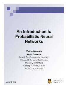
First, some very simple but typical situations will be considered. These situations are depicted in Fig. 1. Dotted circle represent uncertain evidences and dotted lines are uncertain implications. Situation 1: Suppose there is an uncertain evidence e. If e is valid, then it implies a hypothesis h necessarily. In terms of propositional logic, this situation can be expressed by e → h.

8

1

Situation 1: e


Situation 2: e

h

a

Situation 3: e

h

Situation 4:

a

h

Situation 5:

e1

e1

h

e2

~h

h e2

Figure 1: Different simple situation of propositional assumption-based models. The proposition e is considered as an assumption which may be valid or not. Let p(e) be its probability. Modus ponens permits to deduce h if e is valid. Thus, e is an argument for h, and there are no arguments against h. The degrees of support and plausibility for h are therefore dsp(h) = p(e) and dpl(h) = 1. If p(e) is sufficiently close to 1, for example if p(e) = 0.9, then we have sufficient reason to believe that h is true. Situation 2: Suppose now that evidence e holds for sure, but that it implies h only contingently. This can be encoded by two propositional statements e, a → (e → h). In this situation a is an assumption which is only valid with a certain probability p(a). Note that the second statement can also be written as a∧ e → h. Again, a is an argument for h and there are no arguments against h. The degrees of support and plausibility for h are again dsp(h) = p(e) and dpl(h) = 1. This situation changes, if the following statement is added: ∼a

→ (e → ∼h).

1.2


9

Now, ∼a is an argument against h and therefore dpl(h) = 1 − (1 − p(a)) = p(a). In this case support and plausibility are equal. Situation 3: If both the evidence e as well as the implication are uncertain, then the knowledge is encoded simply as a → (e → h). Both propositions e and a are considered as assumptions with probabilities p(e) and p(a). In this situation, both assumptions e and a must be valid in order to deduce h. The set of literals {e, a} is therefore an argument for h. If independence of the assumptions is assumed, then its degree of support is dsp(h) = p(e) · p(a). There are no arguments against h unless a second statement such as ∼a

→ (e → ∼h)

is added. Then, {e, ∼a} is an argument against h and the degree of plausibility of h becomes dpl(h) = 1 − p(e) · (1 − p(a)). Note that support and plausibility are different, but in any case we have dsp(h) ≤ dpl(h). Situation 4: Consider the following situation with two uncertain evidences e1 and e2 , each of them implying the hypothesis h: e1 → h,

e2 → h.

Each ei is considered to be an assumption which holds with probability p(ei ). Every assumption e1 and e2 is then an argument for h. The degree of support for h is the probability that at least one of these arguments is valid, that is dsp(h) = P (e1 ∨ e2 )

= 1 − (1 − p(e1 )) · (1 − p(e2 )).

10

1


This formula shows how multiple evidence enforces the credibility of a hypothesis. The situation becomes more interesting, if we add statements like ∼e1

→ ∼h,

∼e2

→ ∼h.

The remarkable fact is now that either both literals e1 and e2 or both literals ∼e1 and ∼e2 must be valid. All other cases lead to a contradiction. In the first case we have an argument in favor of h, and in the second case an argument against h. Contradictory combinations of assumptions are not possible, since they contradict the given knowledge. Therefore, the results must be conditioned on the fact, that (e1 ∧ e2 ) ∨ (∼e1 ∧ ∼e2 ) must be true. The degree of support of h can then be computed as follows: dsp(h) = P (e1 ∨ e2 |(e1 ∧ e2 ) ∨ (∼e1 ∧ ∼e2 )) P (e1 ∧ e2 ) = P ((e1 ∧ e2 ) ∨ (∼e1 ∧ ∼e2 )) p(e1 ) · p(e2 ) = . p(e1 ) · p(e2 ) + (1 − p(e1 )) · (1 − p(e2 )) The degree of support for ∼h can be determined in a similar way, that is we get dsp(∼h) =

(1 − p(e1 )) · (1 − p(e2 )) . p(e1 ) · p(e2 ) + (1 − p(e1 )) · (1 − p(e2 ))

Note that this situation implies dsp(h) + dsp(∼h) = 1, and consequently we have dsp(h) = dpl(h). Situation 5: The following situation of contradictory evidence must be treated similarly. Suppose that the statements e1 → h,

e2 → ∼h, are given. Here e1 and e2 are considered as assumptions with corresponding probabilities p(e1 ) and p(e2 ). Clearly, e1 is an argument in favor of h, and e2 is an argument against h. Therefore, if both assumptions e1 and e2 are

1.2


11

valid, then a contradictory situation arises. Again, contradictions must be eliminated by conditioning the results. dsp(h) = P (e1 |∼(e1 ∧ e2 )) = =

p(e1 ) · (1 − p(e2 )) . 1 − p(e1 ) · p(e2 )

P (e1 ∧ ∼(e1 ∧ e2 )) P (e1 ∧ ∼e2 ) = P (∼(e1 ∧ e2 )) 1 − P (e1 ∧ e2 )

Contradictory evidence weakens the strengths of belief in the hypothesis. In fact, suppose, for example, p(e1 ) = p(e2 ) = 0.9 such that e1 alone gives h a credibility of 0.9. However, in view of the above formula we obtain only dsp(h) = 0.474. General Situation: Now, consider a more general situation where an arbitrary set of propositional formulae Σ = {ξ1 , ξ2 , . . . , ξn } is given. These formulae contain propositional symbols from two sets A = {a1 , a2 , . . . , an } (assumptions) and P = {p1 , p2 , . . . , pm } (ordinary propositions). Let A± = {a1 , a2 , . . . , an , ∼a1 , ∼a2 , . . . , ∼an } be the set of all literals formed by elements of A. A subset a ⊆ A± is called contradiction, if a together with Σ is not satisfiable. If h is an arbitrary propositional formula, then a subset a ⊆ A± is called quasi-support of h, if a together with Σ entails h, that is a, Σ |= h. The subset a is called support of h, if it is a quasi-support of h, but not a contradiction. If we assume probabilities p(ai ) for the corresponding assumptions ai , then the degree of support of a hypothesis h can be defined as conditional probability dsp(h) = P (a support a of h is valid | no contradiction). Similarly, the plausibility of ∼h can be defined as dpl(h) = P (no support of ∼h is valid | no contradiction). For a rigorous discussion of this formalism we refer to (Kohlas & Monney, 1995).

12

1.3

1


Reasoning with Hints

Assumptions and propositions in propositional logic can be regarded as binary variables. In a generalization of this framework, consider variables with a finite set of possible values. Such a set of possible values is called frame. Again, some variables are considered as assumptions. A hint is defined relative to an assumption A with frame ΩA and another variable X with frame ΘX . A subset Γ(ω) ⊆ ΘX is associated to each possible value ω ∈ ΩA . The values in ΩA are also called interpretations. Furthermore, probabilities p(ω) are given for each value in ΩA such that X

p(ω) = 1.

ω∈ΩA

A hint is thought to represent a body of information relative to a variable X. This body of information is uncertain in the sense that the knowledge about X depends on different possible interpretations ω ∈ ΩA . One of the possible interpretations in ΩA is supposed to be the correct one. If ω happens to be the correct interpretation, then the unknown value of the variable X is known to be in the subset Γ(ω). The subset Γ(ω) is called focal set of ω. For example, consider a certificate of whether an expensive painting is original or faked. Thus, the frame of the variable X is ΘX = {original, f aked}. The expert’s certificate can be interpreted as follows: ω1 : the expert is experienced and not lying, ω2 : the expert is experienced and lying, ω3 : the expert is not experienced. The frame ΩA of possible interpretations is then {ω1 , ω2 , ω3 }. Suppose now that the expert certifies the originality of the painting. If ω1 is assumed to be the correct interpretation, then the conclusion is necessarily that the painting is original, that is Γ(ω1 ) = {original}. If ω2 is assumed, then the conclusion must be Γ(ω2 ) = {f aked}. Finally, if ω3 is assumed, then the expert may be right or wrong, and nothing can be concluded, that is Γ(ω3 ) = {original, f aked} = ΘX . Under this third interpretation the certificate is worthless, since it contains no information about the question of the originality of the painting.

1.3


13

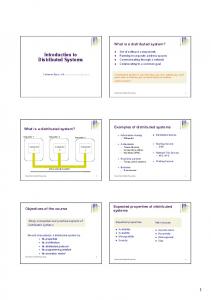
The hint is completed by defining probabilities for the three possible interpretations. These probabilities indicate the confidence we have in the expert. For example, if the expert is judged to be trustworthy, but if there is still some doubt about his expertise, we may set p(ω1 ) = 0.8, p(ω2 ) = 0.01, and p(ω3 ) = 0.19. The given hint is depicted in Fig. 2. 0.8 ω1 ω2 ω3

ΩA

0.01

original faked

0.19

ΘX

Figure 2: Graphical representation of a hint. For a given hint, hypotheses about the variable X may be of interest. A hypothesis about X is defined by a subset H of the frame ΘX . The hypothesis H states that the unknown value of X is contained in H. Which assumptions or interpretations ω ∈ ΩA support this hypothesis? Clearly, every ω such that Γ(ω) ⊆ H is an argument for H since H must necessarily be true, if ω is the correct interpretation. Therefore, the support of H is the set {ω ∈ ΩA : Γ(ω) ⊆ H}. According to this remark, the degree of support for H is the probability that the unknown interpretation supports the hypothesis, that is dsp(H) = P {ω ∈ ΩA : Γ(ω) ⊆ H} =

X

p(ω).

ω∈ΩA : Γ(ω)⊆H

Note that dsp(H) as a function of H ⊆ ΘX is a belief function in the sense of the Dempster-Shafer theory of evidence (Shafer, 1976). An interpretation ω ∈ ΩA supports the complement H c if Γ(ω) ⊆ H c or equivalently, if Γ(ω) ∩ H = Ø. Hence, the degree of plausibility of H can be defined as dpl(H) = P {Γ(ω) ∩ H 6= Ø} = 1 − dsp(H c ). In the example above, only the interpretation ω1 supports the hypothesis H = {original} that the painting is original, that is dsp({original}) = p(ω1) = 0.8. On the other hand, ω2 supports the hypothesis H c = {f aked}

14

1


and therefore we have dsp({f aked}) = p(ω2 ) = 0.01. This implies also that dpl({original}) = 1 − dsp({f aked}) = 0.99. If there is a second hint regarding the same variable X, we need some way to combine it with the first one. Consider then two hints relative to the same variable X with frame ΘX , but with two distinct assumptions A1 and A2 with corresponding frames (possible interpretations) Ω1 and Ω2 . In both hints there must be a correct interpretation, say ω ∈ Ω1 for the first and υ ∈ Ω2 for the second hint. Looking at the two hints simultaneously, the pair (ω, υ) must be the correct combined interpretation. According to the first hint, the unknown value of X must be in the subset Γ1 (ω) and according to the second hint in the subset Γ2(υ). Consequently, the correct value of X must be in the subset Γ(ω, υ) = Γ1 (ω) ∩ Γ2 (υ). Unfortunately, the correct interpretations of the given hints are unknown, but suppose that their probabilities p1 (ω) and p2 (υ) are given. If stochastic independence between the two interpretations is assumed, then we obtain the probabilities p(ω, υ) = p1 (ω) · p2 (υ) of the combined interpretations. Therefore, the combination of the two original hints leads to a new (combined) hint with Ω1 × Ω2 as set of possible interpretations and with probabilities and focal sets as defined above. However, in some cases an additional consideration is necessary. It is possible that a pair of combined interpretations ω, υ from two hints have empty focal sets, that is Γ1 (ω)∩Γ2 (υ) = Ø. Since the variable X must have a value, such pairs do not represent possible combined interpretations. For example, if a second expert also certifies the painting as original, then it is not possible that one of the experts is a liar and the other one says the truth (and both are experienced). In this case one would conclude {original} from one hint and {f aked} from the other one. Clearly, this is contradictory. Contradictory combined interpretations must be eliminated such that the set of possible combined interpretations is defined as Ω = {(ω, υ) : ω ∈ Ω1 , υ ∈ Ω2 , Γ1 (ω) ∩ Γ2 (υ) 6= Ø}. The probabilities of the combined interpretations must then be conditioned on this set. For that purpose let’s define k=

X

(ω,υ)∈Ω

p1 (ω) · p2 (υ).

1.3


15

The probabilities of the combined interpretations in Ω are then p1 (ω) · p2 (υ) , for k > 0. k With this additional element we obtain Dempster’s rule of combination (Dempster, 1967; Shafer, 1976). p(ω, υ) =

As an illustration suppose that the second expert is judged to be less trustworthy but more experienced than the first one. We assume for this second expert p(ω1 ) = 0.6, p(ω2 ) = 0.35, and p(ω3 ) = 0.05. The following table shows the possible combined interpretations, the corresponding focal sets, and their combined probabilities before and after conditioning. Expert 1 ω1 ω1 ω2 ω2 ω3 ω3 ω3

Expert 2 ω1 ω3 ω2 ω3 ω1 ω2 ω3

Focal Set {original} {original} {f aked} {f aked} {original} {f aked} {original, f aked} k=

p1 · p2 0.4800 0.0400 0.0035 0.0005 0.1140 0.0665 0.0095 0.7140

p1 ·p2 k

0.6723 0.0560 0.0049 0.0007 0.1597 0.0931 0.0133

There are three combined interpretations supporting {original} and three others supporting {f aked}. From the table above we can therefore derive dsp({original}) = 0.888, dpl({original}) = 1 − dsp({f aked}) = 1 − 0.0987 = 0.9013. Note that the second certificate reinforces the credibility of the originality of the painting. In contrast, a second contradicting certificate would weaken the credibility. In Chapter 3, more examples of reasoning with hints will be given. For the mathematical background of hints, we refer to (Kohlas & Monney, 1995). Hints can be implemented efficiently with the technique of finite set constraints (Anrig et al., 1997c; Haenni & Lehmann, 1998). An advantage of this approach is that the concept of hints can easily be combined with propositional assumption-based systems (see Section 1.2). As a consequence of this, it is possible to treat mixed models by the same inference mechanism.

16

2

2

ELEMENTS OF ABEL

Elements of ABEL

This chapter describes ABEL (Assumption Based Evidential Language) which is both a modeling language for assumption-based systems and an interactive tool for assumption-based reasoning (Anrig et al., 1997a; Anrig et al., 1997b).1 Given an assumption-based system and some additional facts or observations, the aim of ABEL is to compute symbolic arguments and numerical supports for the user’s hypotheses (see Fig. 1). ??? Hypothesis

Facts and Observations

Expert

User

ABEL 2.2

sp(h,∑) ? Knowledge Base

ABEL 2.2

Hypothesis

0.74

Symbolic & Numerical Arguments

Figure 1: Using ABEL to compute symbolic and numerical arguments.

ABEL was originally designed and implemented at the University of Fribourg for the Macintosh platform. It results from a research project of an extent of several years. The developers are the authors of this publication. The program is written in Common Lisp and CLOS (Common Lisp Object System), and it is therefore easily portable to different platforms. The software can be downloaded from the ABEL homepage: 1

The actual version is ABEL 2.2.

2.1

Introduction

17 http://www-iiuf.unifr.ch/tcs/abel

An introduction to the language, its grammar and a lot of other information, as well as several interactive examples can be accessed on the internet at the same address. Examples of ABEL models can also be found in the Chapter 3 and in (Anrig et al., 1997a).

2.1

Introduction

The language is based on three other computer languages: (1) from Common Lisp (Steele, 1990) it adopts prefix notation and therewith a number of opening and closing parentheses; (2) from Pulcinella (Saffiotti & Umkehrer, 1991) it takes the idea of the commands tell, ask, and empty; and (3) from a former ABEL prototype (Lehmann, 1994; Haenni, 1996) it inherits the concept of modules and the syntax of the queries. Working with ABEL usually involves three sequential steps: 1. The actual information is expressed using the command tell (see Section 2.2). The resulting model is called basic knowledge base. It describes the part of the available information that is relatively constant and static in course of time such as rules, hints, relations, or dependencies between different statements or entities. 2. Actual facts or observations about the concrete, actual situation are specified using the command observe (see Section 2.3). Facts and observations may change in course of time. The basic knowledge base completed by actual observations is called actual knowledge base. 3. Queries about the actual knowledge base are expressed using the command ask. For a given hypothesis, different types of queries are possible (see Section 2.4).

2.2

The Command tell

The most important feature in ABEL is the command tell. It is used to build the basic knowledge base. It consists of one or several lines called instructions. The contents of an instruction can be (1) a definition of types,

18

2

ELEMENTS OF ABEL

variables, assumptions, or modules, (2) a statement, that is a rule or another part of the basic knowledge base, or (3) an instantiation of a module. The sequence of instructions is interpreted in parallel as a conjunction. The order in which the instructions appear within a tell command is therefore not important. The syntax of a tell command is the following: (tell ... )

Every instruction can be seen as a piece of information. Therefore, the command tell is used to add new pieces of information to the existing basic knowledge base. Note that the instructions of a tell command can be distributed among several tell commands. The following sequence of tell commands, for example, is equivalent to the command above: (tell ) (tell ) ... (tell )

Different tell commands are often used to group related pieces of information and to separate these groups from each other. ABEL supports this technique by allowing keywords for specifying different tell commands. A keyword is either a name with a preceding colon (e.g. :part1, :part2, etc.) or an integer. A keyword is always the first argument of a tell command: (tell ... )

Keywords can be used to change or delete different parts of the knowledge base independently (see Section 2.5). In cases of big knowledge bases, this technique turns out to be very useful. It also helps to visualize the structure of the given information.

2.2

The Command tell

2.2.1

19

Type Definitions and Pre-Defined Types

Reasoning under uncertainty is always concerned with open questions. A question is determined by the set of possible answers called frame. An important element of ABEL is therefore the possibility of declaring frames. Note that different questions may have the same frame; they are said to be of the same type. Therefore, ABEL provides a command type to define frames. Such a set may contain symbols or numbers. Examples: (type test (passed failed)) (type colors (red green blue yellow)) (type month (1 2 3 4 5 6 7 8 9 10 11 12))

There are also a few pre-defined types in ABEL: • integer: the set of (positive and negative) integers;

• real: the set of (positive and negative) real numbers;

• binary: a special type to declare propositional symbols. It is also possible to define subsets of pre-defined types such as intervals. Examples: (type (type (type (type (type

year integer) month (integer 1 12)) size (real 0 250)) pos-integer (integer 0 *)) neg-real (real * 0))

The symbol * represents an unbound interval, that is (real 5 *) denotes the real numbers greater than or equal to five. 2.2.2

Variables and Assumptions

The second step consists in defining variables and assumptions. Variables represent questions. ABEL is a typed language, so for each variable, the set of possible values (answers) has to be specified, that is the type of the variable must be declared. Note that different variables can be of the same type. In ABEL, variables are defined as follows:

20

2

ELEMENTS OF ABEL

(var ... )

An individual var command is therefore necessary for each type of variable. The type specifier can either be a pre-defined type, a user-defined type, or a new type specification according to the previous subsection. Examples: (var (var (var (var (var (var (var

c1 c2 colors) a b n integer) x y z real) language (french german spanish english)) s (real 0 250)) pi 3.1416) p q r binary)

Assumptions are defined in a similar way. The difference between assumptions and variables is that assumptions represent uncertain events, unknown circumstances, or risks, rather than precise open questions. Assumptions are used to build arguments for hypotheses. Additionally, it is often possible to impose probabilities on the values of an assumption. The actual version of ABEL supports only probabilities for binary and finite assumptions. The probabilities of different assumptions are assumed to be mutually independent. Specifying probabilities is optional in ABEL. If no probabilities are declared, then a uniform distribution is assumed, that is 0.5 for binary assumptions and n1 for finite assumptions with n possible values. Assumptions can be defined as follows: (ass ... )

The probabilities are given as a list of values between 0 and 1 summing to 1. The order in which the probabilities appear in the list corresponds to the order in which the values for the given type are defined. Examples: (ass (ass (ass (ass

test1 test2 test (0.8 0.2)) weather (sun clouds rain) (0.5 1/3 1/6)) k1 k2 k3 colors) ok? binary 0.75)

In the special case of assumptions of type binary (propositional symbols), only the probability p for the positive literal has to be specified. The probability for the negative literal is given implicitly by 1 − p.

2.2

The Command tell

2.2.3

21

Expressions

Based on numerical variables and assumptions of type integer or real, it is possible to build compound (algebraic) expressions. The syntax of ABEL expressions corresponds to LISP expressions. It uses prefix notation: the first element within a pair of opening and closing parentheses is the name of one of the pre-defined algebraic operators. The remaining elements are the operands, that is names of numerical variables or assumptions: ( ... )

ABEL provides the following algebraic operators: +, -, *, /, sqr, sqrt, exp, expt, log, abs, sin, cos, tan, asin, acos, atan, mod, min, and max. The semantic of these operators corresponds to Common LISP (Steele, 1990). Examples: (+ x y z) (/ (* x y) z) (- (max x y z) (min x y z)) (abs (sin (sqrt x)))

Note that variables (e.g. x, y, c1, language, etc.), assumptions (e.g. test1, test2, weather, ok?, etc.), numbers (e.g. 17, 1/3, -23.5, etc.), symbols (e.g. french, sun, etc.), and sets (e.g. (german spanish), (1 2 4 5 10), etc.) are also considered as (atomic) expressions. Furthermore, there are two pre-defined expressions true and false. 2.2.4

Constraints

ABEL expressions can be used to build so-called constraints. They restrict the possible values of the variables or assumptions involved to a subset of their Cartesian product. Constraints always compare two expressions. The syntax is therefore as follows: ( )

ABEL provides the following operators to build constraints:

22

2 =

ELEMENTS OF ABEL

sets a variable or assumption (1st expression) to a certain value (2nd expression), or restricts the two expressions to be equal;

complement of =; in restricts the possible values of a finite variable or assumption (1st expression) to a subset of the corresponding frame (2nd expression);
= restricts the first (algebraic) expression to be greater or equal than the second (algebraic) expression. Examples: (= c1 blue) (= n 17) ( (+ x y) z) (in language (german spanish)) (< x 23.5) (>= (/ (sin x) (cos x)) (tan x)) ok? (= p true) (= q false)

Note that variables and assumptions of type binary (e.g. ok?, p, q, etc.) are also considered as (atomic) constraints. In this sense, ok? is equivalent to (= ok? true), and (not ok?) is equivalent to (= ok? false). 2.2.5

Statements

Constraints can be used to build logical expressions called statements. A constraint itself is considered as (atomic) statement. ABEL supports the following different types of compound statements:

2.2

The Command tell

23

• (-> ): material implication; • ( ): equivalence; • (and ... ): logical and; • (or ... ): logical (inclusive) or; • (xor ... ): logical exclusive or; • (not ): negation. Examples: (and (= n 17) (= c1 blue)) (-> (= (+ x y) z) (in language (german spanish))) (not (>= (/ (sin x) (cos x)) (tan x))) ok?

Statements are used to build the basic knowledge base. Every single statement describes a part of the given information. A sequence of statements is interpreted as conjunction. The following two statements are therefore equivalent to the first statement of the previous examples: (= n 17) (= c1 blue)

Note that there are two pre-defined constraints: tautology represents a statement that is always true, and contradiction is a statement which is unsatisfiable. These special cases are of particular importance as possible hypotheses in queries (see Section 2.4).

2.2.6

Modules

The idea of modules is that similar parts of the given information are modeled only once. The definition of a module can be compared with the definition of a LISP function. Every module has a name and it consists of a set of parameters and a body. The parameters of an ABEL module are variables or assumptions. The body of a module is a sequence of ABEL instructions

24

2

ELEMENTS OF ABEL

(see Section 2.2). Therefore, it is possible to define local types, local variables, local assumptions, and local modules within the body of a module. The syntax for a module definition is the following: (module ( ... ) ... )

Note that the parameters of a module have to be declared either as variables or assumptions. Additionally, types have to be specified for the parameters. The parameter list is therefore a sequence of variable and assumption definitions (see Subsection 2.2.2). The following example of a module representing an and-gate is taken from Subsection 3.1.3: (tell (module AND-GATE ((var in1 in2 out binary)) (ass ok binary 0.99) (-> ok ( out (and in1 in2))) (-> (not ok) (not ( out (and in1 in2))))))

A module can be used to generate similar parts of the given information. An instance of a module is obtained by “calling” the module with actual parameters. Additionally, a keyword, that is a symbol with preceding colon or a number, can be assigned to each instance of a module. These keywords allow to access locally defined variables from outside a module. This is especially helpful for queries (see Section 2.4). If no keyword is specified, a unique keyword is generated by the system. Modules are instantiated as follows: ( ... ) ( ... )

Note that the types of the actual parameters are implicitly given by the parameter specification of the module definition. It is therefore possible but not necessary to define the actual parameters outside the module. Consider again the example from above. Two instances AND-1 and AND-2 of the module AND-GATE are created by the following code:

2.3

The Command observe

25

(tell (AND-GATE :AND-1 input-1 input-2 output-1) (AND-GATE :AND-2 output-1 input-3 output-2))

The local assumptions ok can then be accessed by AND-1.ok or AND-2.ok.

2.3

The Command observe

To complete a model, observations or facts are added to the basic knowledge base. Observations describe the actual situation or the concrete circumstances of the problem. Note that observations may change in course of time. It is therefore important to separate observations from the basic knowledge base. ABEL provides a command observe to specify observations. It expects a sequence of ABEL statements. The sequence is interpreted as a conjunction. (observe ... )

Examples: (observe (= n 17) (= c1 blue)) (observe (in language (german spanish))) (observe ok?)

Statements given by observe and tell commands are treated similarly. The difference is that observe-statements can be deleted or changed independently when new observations were made (see Section 2.5). Just as for the tell command (see Section 2.2), a keyword can be specified for each observe command: (observe ... )

26

2

ELEMENTS OF ABEL

These keywords allow then to change observations individually using the empty command (see Section 2.5). Example: (observe :first-observation (= n 17) (in language (german spanish))) (empty :first-observation) (observe :updated-observation (= n 19) (= language german))

Note that it is not possible to delete independently observations without keywords. They can only be deleted together with all observations or the whole knowledge base (see Section 2.5).

2.4

The Command ask

Queries about the actual knowledge base are expressed using the command ask. Generally, there are two different types of queries: (1) it can be interesting to get the available information about certain variables, (2) it can be interesting to get a qualitative or a quantitative judgment of a hypothesis. In both cases, several queries can be treated within the same command: (ask ... )

In the first case, a query is simply an ABEL expression in the sense of Subsection 2.2.3. This type of query is useful for questions like “what do we know about the variable X” or “what do we know about the variables X and Y ”. Examples:

2.4

The Command ask

27

(ask language) (ask (x y)) (ask (+ x y z))

The second way to state queries is important in problems of assumptionbased reasoning. The idea is to find arguments in favor or against hypotheses. For a given hypothesis, different types of arguments may be of interest: support, quasi-support, plausibility, or doubt (for further information on this we refer to (Haenni, 1996), (Kohlas & Besnard, 1995), etc.). A hypothesis is an ABEL statement in the sense of Subsection 2.2.5: (sp (qs (pl (db

) ) ) )

Examples: (ask (sp (and (= n 17) (< x 5)))) (ask (pl (in language (german spanish))) (db (not ok?)))

Arguments are minimal conjunctions of ordinary or negated ABEL constraints over assumptions. The support of a hypothesis, for example, is the set of all such minimal conjunctions (built of assumptions), which allow to deduce the hypothesis from the given knowledge base. Such a set set is presented as a list with each conjunction on one line, for example: 52.9% : OK? (= TEST1 PASSED) 47.1% : (= K1 RED) (= K2 GREEN)

The above result consists of two arguments. The percentage on the lefthand side of each line specifies the importance of the explanation. Note that these percentages do not coincide with the posterior probabilities of the explanations. If probabilities are specified for all assumptions, then these percentages reflect the normalized2 prior probabilities of the respective 2

Normalized means in this context that the sum of the percentages must be 1.

28

2

ELEMENTS OF ABEL

explanation. If no probabilities are specified then a uniform probability distribution is assumed to calculate the percentages. It is also possible to ask for numerical arguments like degree of support, degree of plausibility, or degree of doubt (Haenni, 1996): (dsp ) (dpl ) (ddb )

A numerical argument is obtained by computing the probability for the corresponding symbolic argument. This computation is based on a priori probabilities given by the definition of the assumptions (Bertschy & Monney, 1996; Kohlas et al., 1998a; Monney & Anrig, 1998).

2.5

Other Facilities

Sometimes, it is necessary to delete the entire knowledge base or parts of it. For that purpose, ABEL provides the command empty. If empty is called without arguments, then the entire model is deleted. If the keyword observe is supplied, then it deletes only the observations. Additionally, by supplying one or several keywords used within tell or observe commands, it is possible to delete only the corresponding parts of the knowledge base. Examples: (empty) (empty observe) (empty :part1 :part2) (empty :updated-observation)

To obtain more readable ABEL models, it is possible to introduce comments into the code. According to Common LISP, there are two different ways for introducing comments: #| This is a comment over one or several lines |# ; This is another comment

29

3

Applications

The aim of this chapter is to show the wide-ranging possibilities of using probabilistic argumentation systems such as ABEL. The following examples are grouped under the headings of model-based prediction and diagnostics, causal modeling and uncertain systems, and evidential reasoning. All the examples include a description of a concrete situation, the corresponding ABEL model, as well as a discussion of some interesting queries.

3.1

Model-Based Prediction and Diagnostics

The problem of technical systems (airplanes, nuclear power stations, television sets, cars, computers, etc.) is that a correct functioning can not be guaranteed. In this sense, technical systems are more or less unreliable. The degree of the reliability depends on different factors like the quality, the age, the complexity, the maintenance, and the service of the system. For a given technical system, two important questions are of interest: (1) How reliable is the system? (Prediction) (2) Which is the component to be repaired or replaced when the system is not working correctly? (Diagnostics) If a complete description or a model of the system’s functionality is given, then argumentation systems can help answering the above questions. The following subsections discuss a number of concrete examples of model-based prediction and diagnostics.

3.1.1

Communication Networks

Propositional assumption-based systems are well suitable for computing reliabilities of communication networks (Kohlas, 1987). Such a network is composed of nodes which are connected by communication wires. If one or several nodes or wires are broken, then some point-to-point connections may be impossible. In such a case, the system is not functioning according to its communication functionality between the two nodes.

30

3

APPLICATIONS

More generally, a system whose actual state is classified as functioning or not functioning is called a binary system. If a broken component of a binary system is always reducing the reliability of the entire system, then the system is called monotone. This condition seems to be reasonable for most cases. In fact, communication networks are monotone systems, since a broken node or wire is always decreasing the network reliability.

x w5

w4

u w0

y w2

w7

w

a

w9

w6

b

w3

w1

w8

v Figure 1: Example of a communication network. Communication networks can be described by directed or undirected graphs. For example, consider a communication network consisting of the nodes a, b, u, v, w, x, and y as shown in Fig. 1. The nodes are connected by wires w0 , w1 , . . . , w9 . A point-to-point communication has to be guaranteed between the nodes a and b. The reliability for this depends on the failure probabilities of the network components. For the purpose of simplification, we suppose that only the communication wires can break down, that is p(ok(a)) = p(ok(b)) = · · · = 1. Furthermore, we assume the following independent probabilities for the wires (instead of p(ok(wi )) we write p(oki )): p(ok0 ) = 0.6, p(ok4 ) = 0.5, p(ok8 ) = 0.2,

p(ok1 ) = 0.9, p(ok5 ) = 0.8, p(ok9 ) = 0.7.

p(ok2 ) = 0.9, p(ok6 ) = 0.9,

p(ok3 ) = 0.3, p(ok7 ) = 0.4,

Note that some of the communication wires (that is w1 , w2 , w3, w6 , w9 ) are bi-directed, whereas others (that is w0 , w4 , w5, w7 , w8 ) are directed. The problem of the given example is to compute the reliability of the communication between the nodes a and b. For that purpose, at least one of the

3.1


31

possible communication paths between a and b must be intact. Examples of communication paths are w1–w8, w0 –w2 –w7 , w0–w2–w3 –w8 , etc. The problem of computing the reliability of the network can therefore be divided into two sequential steps: (1) Determine all possible communication paths; (2) Derive the network reliability from the set of possible communication paths and the given failure probabilities. In ABEL, this corresponds to the idea of computing first a symbolic and in a second step the numerical solution. In fact, communication networks can easily be modeled in ABEL. The example above can be expressed in ABEL by defining binary variables for the nodes and binary assumptions with corresponding probabilities for the wires: (tell (var (ass (ass (ass (ass (ass (ass (ass (ass (ass (ass

a b ok0 ok1 ok2 ok3 ok4 ok5 ok6 ok7 ok8 ok9

u v w x y binary) binary 0.6) binary 0.9) binary 0.9) binary 0.3) binary 0.5) binary 0.8) binary 0.9) binary 0.4) binary 0.2) binary 0.7))

The network itself can then be modeled by implications of the form oki → (n1 → n2 ) for each directed communication wire, and oki → (n1 ↔ n2) for each bi-directed communication wire: (tell (-> (-> (-> (-> (-> (-> (->

ok0 ok1 ok2 ok3 ok4 ok5 ok6

(-> a u)) ( a v)) ( u w)) ( v w)) (-> u x)) (-> x y)) ( w y))

32

3

APPLICATIONS

(-> ok7 (-> w b)) (-> ok8 (-> v b)) (-> ok9 ( y b)))

Then, the interesting question is, if a message m from node a is also accessible at node b. The answer for this question is obtained by the following ABEL query: ? (ask (sp QUERY: (SP 24.6% : 15.6% : 13.0% : 12.3% : 12.2% : 7.8% : 6.3% : 4.9% : 2.3% : 0.9% :

(-> (-> OK0 OK0 OK1 OK1 OK0 OK1 OK0 OK1 OK0 OK0

a b))) A B)) OK2 OK6 OK2 OK7 OK8 OK3 OK6 OK4 OK5 OK3 OK7 OK4 OK5 OK2 OK3 OK2 OK3 OK3 OK4

OK9

OK9 OK9 OK6 OK7 OK4 OK5 OK9 OK8 OK5 OK6 OK8

The resulting arguments can be interpreted as possible minimal communication paths between a and b. The reliability of the network is then obtained by the corresponding numerical query: ? (ask (dsp (-> a b))) QUERY: (DSP (-> A B)) 0.623

This result can be interpreted as the probability for the message m to be passed from a to b assuming that the communication wires are breaking down according to the given failure probabilities. In a similar way, it is possible to compute the reliability for the inverse communication between b and a: ? (ask (sp (-> b a))) QUERY: (SP (-> B A)) 100.0% : OK1 OK3 OK6 OK9

3.1


33

? (ask (dsp (-> b a))) QUERY: (DSP (-> B A)) 0.170

Obviously, there is only one possible communication path from b to a (see Fig. 1), and a communication from b to a is therefore much more unreliable than from a to b (0.17 instead of 0.623). Now, suppose that a failure of the communication wire w3 between v and w is detected. In ABEL this can be expressed as follows: (observe (not w3))

Again, the interesting question is the reliability of the communication between a and b and inversely: ? (ask (dsp (-> a b))) QUERY: (DSP (-> A B)) 0.548 ? (ask (dsp (-> b a))) QUERY: (DSP (-> B A)) 0.000

Note that compared to the situation above the reliability for a communication from a to b has decreased slightly, while a communication from b to a is now completely unreliable (i.e. impossible). Suppose now that the broken wire w3 between v and w is replaced. If a correct functioning of the new wire is assumed, then we can write the following ABEL commands: (empty observe) (observe ok3)

Clearly, the communication reliabilities have increased for this new situation. ? (ask (dsp (-> a b))) QUERY: (DSP (-> A B))

34

3

APPLICATIONS

0.799 ? (ask (dsp (-> b a))) QUERY: (DSP (-> B A)) 0.567

Consider now another situation where a communication break-down between a and b is observed. The problem then is to compute possible diagnoses explaining the error. (empty observe) (observe (not (-> a b)))

The set of possible diagnoses is then obtained by the following query: ? (ask (sp QUERY: (SP 44.2% : 28.4% : 7.9% : 5.5% : 4.7% : 2.5% : 2.2% : 1.9% : 1.0% : 0.4% : 0.4% : 0.4% : 0.3% : 0.2% : 0.1% :

tautology)) TAUTOLOGY) (NOT OK0) (NOT (NOT OK7) (NOT (NOT OK0) (NOT (NOT OK2) (NOT (NOT OK4) (NOT (NOT OK1) (NOT (NOT OK2) (NOT (NOT OK5) (NOT (NOT OK1) (NOT (NOT OK1) (NOT (NOT OK1) (NOT (NOT OK0) (NOT (NOT OK2) (NOT (NOT OK1) (NOT (NOT OK1) (NOT

OK3) OK8) OK1) OK3) OK6) OK3) OK3) OK6) OK2) OK3) OK2) OK2) OK3) OK3) OK2)

(NOT OK8) (NOT OK9) (NOT (NOT (NOT (NOT (NOT (NOT (NOT (NOT (NOT (NOT (NOT (NOT

OK4) OK7) OK7) OK5) OK7) OK4) OK4) OK5) OK6) OK6) OK5) OK6)

(NOT (NOT (NOT (NOT (NOT

OK8) OK8) OK9) OK8) OK8)

(NOT OK6) (NOT OK7) (NOT (NOT (NOT (NOT

OK7) (NOT OK8) OK8) (NOT OK9) OK6) (NOT OK7) OK9)

Every resulting diagnosis can be considered as a cut between the nodes a and b (Kohlas, 1987). The first diagnosis, for example, tells us that a communication between a and b fails when the point-to-point communications between a and u, between v and w, and between v and b fail simultaneously (see Fig. 1). Note that this is the most probable explanation of the observed communication break-down. Another probable explanation is the second one, while the other explanations are rather unprobable.

3.1


35

To get a better idea of the faulty point-to-point communications, let’s examine the results of the following numerical queries: ? (ask (dsp (dsp (dsp (dsp QUERY: (DSP 0.689 QUERY: (DSP 0.145 QUERY: (DSP 0.141 QUERY: (DSP 0.840 QUERY: (DSP 0.527 QUERY: (DSP 0.211 QUERY: (DSP 0.133 QUERY: (DSP 0.720 QUERY: (DSP 0.973 QUERY: (DSP 0.474

(not (not (not (not (NOT

ok0)) (dsp (not ok1)) (dsp (not ok2)) ok3)) (dsp (not ok4)) (dsp (not ok5)) ok6)) (dsp (not ok7)) (dsp (not ok8)) ok9))) OK0))

(NOT OK1)) (NOT OK2)) (NOT OK3)) (NOT OK4)) (NOT OK5)) (NOT OK6)) (NOT OK7)) (NOT OK8)) (NOT OK9))

Given these degrees of support, it is reasonable to check or repair some of the communication wires, especially those with values > 0.5, that is the wires w8 , w3, w7 , w0 , and w4 (see Fig. 1). Again, suppose that the wire w3 between v and w is replaced and that the new wire is assumed to be intact: (observe ok3)

If the communication break-down between a and b is still observed after the replacement, then the new set of possible diagnoses can be computed as before: ? (ask (sp tautology))

36

3

QUERY: (SP 63.5% : 17.6% : 10.6% : 4.2% : 2.2% : 0.9% : 0.8% :

TAUTOLOGY) OK3 (NOT OK7) OK3 (NOT OK0) OK3 (NOT OK4) OK3 (NOT OK5) OK3 (NOT OK1) OK3 (NOT OK1) OK3 (NOT OK0) (NOT OK8) 0.1% : OK3 (NOT OK1)

(NOT (NOT (NOT (NOT (NOT (NOT (NOT

OK8) OK1) OK6) OK6) OK2) OK2) OK2)

APPLICATIONS

(NOT OK9) (NOT (NOT (NOT (NOT (NOT

OK7) (NOT OK8) OK7) (NOT OK8) OK4) OK5) OK6) (NOT OK7)

(NOT OK2) (NOT OK6) (NOT OK9)

The situation has now changed: the best explanation tells us that all the incoming wires of b must be faulty. This is clearly the most probable explanation and it is therefore reasonable to check or repair these wires. To get a confirmation for this, consider the new values of the numerical queries: ? (ask (dsp (dsp (dsp (dsp QUERY: (DSP 0.495 QUERY: (DSP 0.263 QUERY: (DSP 0.116 QUERY: (DSP 0.000 QUERY: (DSP 0.536 QUERY: (DSP 0.214 QUERY: (DSP 0.188 QUERY: (DSP 0.913 QUERY: (DSP 0.957 QUERY: (DSP 0.750

(not (not (not (not (NOT

ok0)) (dsp (not ok1)) (dsp (not ok2)) ok3)) (dsp (not ok4)) (dsp (not ok5)) ok6)) (dsp (not ok7)) (dsp (not ok8)) ok9))) OK0))

(NOT OK1)) (NOT OK2)) (NOT OK3)) (NOT OK4)) (NOT OK5)) (NOT OK6)) (NOT OK7)) (NOT OK8)) (NOT OK9))

3.1


3.1.2

37

Availability of Energy Distribution Systems

The function of an energy distribution system as depicted in Fig. 2 is to supply a high-tension line L3 from one of two incoming high-tension lines L1 and L2 over the bus A1 (Kohlas, 1987). The lines L1 , L2 , and L3 are protected by corresponding high-tension switches S1 , S2 , and S3. In case of a broken switch it is possible to redirect the electric current on a second bus A2 which is protected by another high-tension switch S4 . The corresponding switches T1 , T2 , and T3 can only be manipulated if no tension is present. L1

L2

S1

S2

A1 T1

T2

S4

A2 S3

T3

L3

Figure 2: Example of an energy distribution system. The energy distribution system is considered to be operating if L3 is linked to L1 or L2 over at least one protecting high-tension switch Si . The problem is to determine the availability of an operating system. The lines L1 , L2 , and L3 have one binary attribute (tension yes/no) and the switches have two attributes (state on/off, intact yes/no). It is uncertain whether the switches are intact or faulty. For that purpose, we assume the following probabilities: p(intact(Si )) = 0.8,

i = 1, 2, 3, 4,

p(intact(Ti )) = 0.95,

i = 1, 2, 3.

38

3

APPLICATIONS

The attributes of the lines and switches can then be modeled by the following definitions of binary variables and assumptions: (tell (var (var (ass (ass

L1 L2 S1 S2 OK-S1 OK-T1

L3 A1 S3 S4 OK-S2 OK-T2

A2 binary) T1 T2 T3 binary) OK-S3 OK-S4 binary 0.8) OK-T3 binary 0.95))

; ; ; ;

tension (yes/no) state (on/off) intact (yes/no) intact (yes/no)

The energy can only pass through a switch if the switch is on and intact. The circuit shown in Fig. 2 can therefore be modeled by the following implications: (tell (-> (and L1 S1 OK-S1) A1) (-> (and L1 T1 OK-T1) A2) (-> (and L2 S2 OK-S2) A1) (-> (and L2 T2 OK-T2) A2) (-> (and A1 S3 OK-S3) L3) (-> (and A2 T3 OK-T3) L3) (-> (and A1 S4 OK-S4) A2) (-> (and A2 S4 OK-S4) A1))

We assume that T1 , T2 , and T3 are only switched on if the corresponding high-tension switches S1 , S2 , and S3 are faulty. Furthermore, we suppose that all the high-tension switches are on. (tell (-> (not OK-S1) T1) (-> (not OK-S2) T2) (-> (not OK-S3) T3) (and S1 S2 S3 S4))

Another important part of the model is the fact that T1 and T3 as well as T2 and T3 are not allowed to be switched on at the same time, because this would supply L3 without protection.

3.1


39

(tell (not (and T1 T3)) (not (and T2 T3)))

Finally, suppose that the incoming lines L1 and L2 are under tension: (observe L1 L2)

The model is now complete and we are interested in the reliability of L3 being under tension. In a first step, this question can be treated by the following symbolic query: ? (ask (sp QUERY: (SP 21.5% : 21.5% : 20.4% : 20.4% : 16.2% :

L3)) L3) OK-S1 OK-S2 OK-S3 OK-S3 OK-S1

OK-S3 OK-S3 OK-S4 OK-T2 OK-S4 OK-T1 OK-S2 OK-S4 OK-T3

The resulting arguments can be interpreted as possible minimal paths of the electric current passing from either L1 or L2 to L3 . The reliability of the entire system is then given by the corresponding numerical query: ? (ask (dsp L3)) QUERY: (DSP L3) 0.960

The following table summarizes the numerical results for different values of p(intact(Si )) and p(intact(Ti )).

p(intact(Ti ))

0 0.2 0.4 0.6 0.8 1

0 0 0 0 0 0 0

0.2 0.31 0.36 0.39 0.42 0.44 0.45

p(intact(Si )) 0.4 0.6 0.52 0.68 0.57 0.73 0.62 0.77 0.66 0.81 0.69 0.84 0.71 0.87

0.8 0.83 0.86 0.89 0.92 0.94 0.96

1 1 1 1 1 1 1

40

3

APPLICATIONS

The table shows that of the high-tension switches Si are dominant and they are therefore much more important for the availability of the system.

3.1.3

Diagnostics of Digital Circuits

Consider the digital circuit for a binary adder as shown in Fig. 3. The system consists of five components: the logical gates and1 , and2 , xor1 , xor2 , and or. The input and output values of the components are the logical values true and f alse (interpreted as 1 and 0). If every component is assumed to work correctly, then the actual input and output values of the binary adder (see Fig. 3) are in conflict with the expected behavior. Therefore, one or several components must be faulty, and the question is which ones. in1 = 1 in2 = 0

xor1

v1 xor2

sum = 1 [0]

or

carry = 0 [1]

and2

inc = 1

v2 v3

and1

Figure 3: Digital circuit of a binary adder.

Suppose that each component has exactly two different operating modes, which are characterized by a binary predicate ok. A correct functioning component means that ok is true, whereas a faulty component implies that ok is false (respectively ∼ok is true). Figure 4 shows an and-gate with two inputs in1 and in2 and one output out. in1

and

out

in2

Figure 4: A simple and-gate.

3.1


41

Suppose that only the behavior of a correct functioning component is known, whereas the error mode is not further specified. An and-gate can then be described as follows (see Fig. 4): ok → (out ↔ in1 ∧ in2 ). All other components of the system are treated similarly. Suppose that the probability for a correct functioning component is 0.99 for and-gates, 0.98 for or-gates, and 0.95 for xor-gates. For each type of component, a corresponding module is defined in ABEL: (tell (module AND-GATE ((var in1 in2 out binary)) (ass ok binary 0.99) (-> ok ( out (and in1 in2)))) (module OR-GATE ((var in1 in2 out binary)) (ass ok binary 0.98) (-> ok ( out (or in1 in2)))) (module XOR-GATE ((var in1 in2 out binary)) (ass ok binary 0.95) (-> ok ( out (xor in1 in2)))))

According to the circuit topology of Fig. 3, another module for the entire adder can be modeled as follows: (tell (module ADDER ((var in1 in2 inc sum carry binary)) (var ok binary) (var v1 v2 v3 binary) (AND-GATE :AND1 (AND-GATE :AND2 (XOR-GATE :XOR1 (XOR-GATE :XOR2 (OR-GATE :OR v2

in1 in2 v3) inc v1 v2) in1 in2 v1) inc v1 sum) v3 carry)

( ok (and AND1.ok AND2.ok XOR1.ok XOR2.ok OR.ok))))

This module is instantiated with the actual variables (Fig. 3):

42

3

APPLICATIONS

(tell (ADDER :ADDER in1 in2 inc sum carry))

Note that it is not necessary to explicitly declare all of the variables used in the model. The types of the variables are determined according to their first occurrence in a module call. For example, in1 (in the instantiation of the adder :ADDER) is a binary variable as defined within the module ADDER. Finally, the ABEL model is completed by the input and output values of the system as shown in Fig. 3: (observe in1 (not in2) inc sum (not carry))

A diagnosis for the system’s behavior is a combination of faulty and correct components, such that the observed input and output values are not in contradiction with the knowledge base (Haenni, 1996). Possible diagnoses are produced by the following query: ? (ask (sp QUERY: (SP 97.1% : 1.9% : 1.0% :

(not (NOT (NOT (NOT (NOT

ADDER.ok))) ADDER.OK)) ADDER.XOR1.OK) ADDER.OR.OK) (NOT ADDER.XOR2.OK) ADDER.AND2.OK) (NOT ADDER.XOR2.OK)

There are three different minimal diagnoses. The first one seems to be the most important one, since it explains the faulty behavior of the systems with only one faulty component. The following numerical queries confirms this result: ? (ask (dsp ADDER.XOR1.ok) (dsp ADDER.XOR2.ok) (dsp ADDER.AND1.ok) (dsp ADDER.AND2.ok) (dsp ADDER.OR.ok)) QUERY: (DSP ADDER.XOR1.OK) 0.028 QUERY: (DSP ADDER.XOR2.OK) 0.924 QUERY: (DSP ADDER.AND1.OK) 0.990 QUERY: (DSP ADDER.AND2.OK) 0.981 QUERY: (DSP ADDER.OR.OK) 0.962

3.1


43

The xor1 -gate is most probably the faulty component of the system and should therefore be replaced. Note that a module for a simple 1-bit adder can be used for building other, more complex systems. For example, two 1-bit adders can be used for a 2-bit adder. Similarly, two 2-bit adders can be used for a 4-bit adder, and so on. In this sense, 2-bit and 4-bit adders can be modeled as follows: (tell (module ADDER2 ((var in1 in2 in3 in4 inc sum1 sum2 carry binary)) (var ok v binary) (ADDER :A1 in1 in2 inc sum1 v) (ADDER :A2 in3 in4 v sum2 carry) ( ok (and A1.ok A2.ok)))) (tell (module ADDER4 ((var in1 in2 in3 in4 in5 in6 in7 in8 inc sum1 sum2 sum3 sum4 carry binary)) (var ok v binary) (ADDER2 :A21 in1 in2 in3 in4 inc sum1 sum2 v) (ADDER2 :A22 in5 in6 in7 in8 v sum3 sum4 carry) ( ok (and A21.ok A22.ok))))

Further modules for 8-bit and 16-bit adders are modeled similarly. Consider now the situation where a modular 16-bit adder is faulty. Suppose that all input and output values are 0, except the value of the last output out16 is 1. (tell (ADDER16 :ADDER16 in01 in02 in03 in04 in05 in06 in11 in12 in13 in14 in15 in16 in21 in22 in23 in24 in25 in26 in31 in32 inc sum01 sum02 sum03 sum04 sum05 sum09 sum10 sum11 sum12 sum13 (observe (not in01) (not in06) (not in11) (not in16)

(not (not (not (not

in02) in07) in12) in17)

(not (not (not (not

in03) in08) in13) in18)

in07 in08 in09 in10 in17 in18 in19 in20 in27 in28 in29 in30 sum06 sum07 sum08 sum14 sum15 sum16 carry))

(not (not (not (not

in04) in09) in14) in19)

(not (not (not (not

in05) in10) in15) in20)

44

3

(not (not (not (not (not (not (not

APPLICATIONS

in21) (not in22) (not in23) (not in24) (not in25) in26) (not in27) (not in28) (not in29) (not in30) in31) (not in32) (not inc) sum01) (not sum02) (not sum03) (not sum04) (not sum05) sum06) (not sum07) (not sum08) (not sum09) (not sum10) sum11) (not sum12) (not sum13) (not sum14) (not sum15) carry) sum16)

ABEL computes then 47 possible minimal diagnoses. The most important results are the following: ? (ask (sp QUERY: (SP 35.2% : 35.2% : 14.1% : 7.0% : 7.0% : ...

(not (NOT (NOT (NOT (NOT (NOT (NOT

ADDER16.ok))) ADDER16.OK)) ADDER16.A82.A42.A22.A2.XOR2.OK) ADDER16.A82.A42.A22.A2.XOR1.OK) ADDER16.A82.A42.A22.A1.OR.OK) ADDER16.A82.A42.A22.A1.AND2.OK) ADDER16.A82.A42.A22.A1.AND1.OK)

Again, numerical results can help to get a better judgment of the situation: ? (ask (dsp (dsp (dsp (dsp (dsp QUERY: (DSP 0.371 QUERY: (DSP 0.371 QUERY: (DSP 0.148 QUERY: (DSP 0.074 QUERY: (DSP 0.074

(not (not (not (not (not (NOT

ADDER16.A82.A42.A22.A2.XOR2.ok)) ADDER16.A82.A42.A22.A2.XOR1.ok)) ADDER16.A82.A42.A22.A1.OR.ok)) ADDER16.A82.A42.A22.A1.AND2.ok)) ADDER16.A82.A42.A22.A1.AND1.ok))) ADDER16.A82.A42.A22.A2.XOR2.OK))

(NOT ADDER16.A82.A42.A22.A2.XOR1.OK)) (NOT ADDER16.A82.A42.A22.A1.OR.OK)) (NOT ADDER16.A82.A42.A22.A1.AND2.OK)) (NOT ADDER16.A82.A42.A22.A1.AND1.OK))

Now, suppose in a more elaborated model that explicit knowledge about one or several fault modes of a component is given. This can easily be modeled in ABEL. For example, consider an and-gate with three different possible fault modes:

3.1


45

st0 : the output is always 0 (stuck at 0), st1 : the output is always 1 (stuck at 1), inv: the output is always the negation of the correct output (inversion). A new variable type can be created to deal with this kind of operating modes. The domain of the variable consists of the fault modes together with the correct operating mode ok: (tell (type modes (ok st0 st1 inv)))

Assume that the probabilities for ok, st0 , st1 , and inv are 0.93, 0.01, 0.01, and 0.05, respectively. The corresponding module in ABEL can then be written as: (tell (module AND-GATE ((var in1 in2 out binary)) (ass mode modes (0.93 0.01 0.01 0.05)) (-> (= mode ok) ( out (and in1 in2))) (-> (= mode st0) (not out)) (-> (= mode st1) out) (-> (= mode inv) ( out (not (and in1 in2))))))

Similar modules can be defined for the other components. It is then possible to compute more precise diagnoses.

3.1.4

Diagnostics of Arithmetical Networks

In the previous subsection, a digital circuit consisting of binary variables has been considered. Now, the more general case of integer variables will be discussed. The following example has been introduced in (Davis, 1984). Subsequently, it was used in several papers on model-based diagnostics (Reiter, 1987; De Kleer & Williams, 1987; Kohlas et al., 1998a). The network consists of three multipliers m1 , m2 , m3 , and two adders a1 , a2. These components are connected as shown in Fig. 5. If only one failure mode is assumed, then a binary variable ok can be used to represent the

46

3 a=3

in1 in2

m1

out

x in1

b=2

c =2

in2

in1 in2

m2

out

out f = 10 [12]

in1 in2

in1 in2

a1

y

d=3

e =3

APPLICATIONS

m3

a2

out g = 12 [12]

out z

Figure 5: An arithmetical network. two modes of the components. The behavior of an adder, for example, can then be expressed by ok → (out = in1 + in2 ). Again, the behavior of a faulty component is not explicitly specified. In ABEL, a module is defined for each type of component. The reliability of a component is modeled by an assumption ok. We assume a probability 0.95 for adders and 0.97 for multipliers. (tell (module ADDER ((var in1 in2 out integer)) (ass ok binary 0.97) (-> ok (= out (+ in1 in2)))) (module MULTIPLIER ((var in1 in2 out integer)) (ass ok binary 0.95) (-> ok (= out (* in1 in2))))

Next, the modules are instantiated according to the network topology of Fig. 5. (tell (MULTIPLIER :M1 a c x)

3.1


47

(MULTIPLIER :M2 b d y) (MULTIPLIER :M3 c e z) (ADDER :A1 x y f) (ADDER :A2 y z g) (var ok binary) ( ok (and M1.ok M2.ok M3.ok A1.ok A2.ok)))

The global variable ok reflects the state of the whole system. Following the example presented in (De Kleer & Williams, 1987), we first consider the situation where only the input measurements are available. (observe (= a 3) (= b 2) (= c 2) (= d 3) (= e 3))

The observed values do not imply that some components are faulty. Therefore, we get the following trivial solution: ? (ask (sp QUERY: (SP 23.8% : 23.8% : 23.8% : 14.3% : 14.3% :

(not (NOT (NOT (NOT (NOT (NOT (NOT

ok))) OK)) M3.OK) M2.OK) M1.OK) A2.OK) A1.OK)

Now, the output value f = 10 is observed: (observe (= f 10))

This measurement together with the given knowledge implies that at least one component is faulty. Three possible minimal diagnoses of this situation are obtained by ABEL: ? (ask (sp QUERY: (SP 38.5% : 38.5% : 23.1% :


ok))) OK)) M2.OK) M1.OK) A1.OK)

48

3

APPLICATIONS

The problem is that the three result are more or less equally important (the percentages are nearly the same). This changes if a further measurement is supplied. Suppose that the value g = 12 is added to the model: (observe (= g 12))

Now, four (more precise) minimal diagnoses are computed: ? (ask (sp QUERY: (SP 59.5% : 35.7% : 3.0% : 1.8% :

(not (NOT (NOT (NOT (NOT (NOT

network-ok))) NETWORK-OK)) M1.OK) A1.OK) M2.OK) (NOT M3.OK) A2.OK) (NOT M2.OK)

Note that two resulting diagnoses are rather unprobable. The faulty component is therefore either the multiplier m1 or the adder a1 . A confirmation of this is obtained by the following numerical queries: ? (ask (dsp (dsp QUERY: (DSP 0.609 QUERY: (DSP 0.092 QUERY: (DSP 0.076 QUERY: (DSP 0.365 QUERY: (DSP 0.046

(not M1.ok)) (dsp (not M2.ok)) (dsp (not M3.ok)) (not A1.ok)) (dsp (not A2.ok))) (NOT M1.OK)) (NOT M2.OK)) (NOT M3.OK)) (NOT A1.OK)) (NOT A2.OK))

To discriminate between m1 and a1 , a further measurement is made for the variable x (see (Anrig, 1998) for a discussion and further literature on how to select such a variable): (observe (= x 6))

Only three minimal diagnoses remain, and only one of them has a high probability:

3.1


? (ask (sp QUERY: (SP 88.2% : 7.4% : 4.4% :


49

ok))) OK)) A1.OK) M2.OK) (NOT M3.OK) A2.OK) (NOT M2.OK)

The first adder is most probably the faulty component. Again, a confirmation for this can be obtained by numerical queries: ? (ask (dsp (dsp QUERY: (DSP 0.050 QUERY: (DSP 0.157 QUERY: (DSP 0.116 QUERY: (DSP 0.887 QUERY: (DSP 0.070

3.1.5

(not M1.ok)) (dsp (not M2.ok)) (dsp (not M3.ok)) (not A1.ok)) (dsp (not A2.ok))) (NOT M1.OK)) (NOT M2.OK)) (NOT M3.OK)) (NOT A1.OK)) (NOT A2.OK))

Failure Trees

The concept of failure trees (or event trees) can help to determine possible causes of a system failure, and it provides a useful structure for the computation of the probability of the system’s working mode. In the case of an ordinary tree, the possible causes are rather easy to detect. But in the literature, the term failure tree is somewhat misleading because in general, the structure considered is a causal network and not a tree. In this more general case, the computation of the causes is more difficult. The failure tree of the following medical example was originally modeled in (Simonaitus et al., 1972) and described in (Barlow & Proschan, 1975). The purpose is to analyze the electrical shock hazard to a patient using a certain heart assist device: “The intra-aortic balloon (IAB) circulatory assist device is intended to provide temporary circulatory assistance following ob-

50

3

APPLICATIONS

struction of blood circulation from the heart. In its application, a balloon-catheter positioned in the thoracic aorta is synchronously inflated and deflated with the action of the heart, resulting in decreased heart work, increased coronary blood flow, and support of the general circulation. A synchronization of the balloon with the heart is obtained through monitoring of the electrocardiogram (ECG) of the patient by a control console. This console provides all of the control, monitoring display, and alarm functions required for operation of the balloon device. In addition, provision is made for automatic deflation of the balloon in the event of an anomaly in the ECG signal or functioning of the balloon. A major hazard to the patient is electrical shock, either macroshock or microshock. Macroshock can cause heart failure (ventricular fibrillation) by currents entering the body through connections at the skin. Microshock can cause heart failure by currents having a conductive path directly to the vicinity of the heart. Other hazards to the patient are balloon inflation during the contraction period of heart function and balloon overpressurization.” A detailed structure of the example is shown in Fig. 6. Note that the example is only treated partially here. In order to reduce the tree’s complexity, some terminal nodes have been introduced for hiding some subtrees. The abbreviations for the nodes introduced in the figure (e.g. HP0 for the top node) will be used in the ABEL model in order to keep the source code readable. The structure of the tree of Fig. 6 can easily be implemented in ABEL. The terminal nodes of the tree are modeled as binary assumptions, and the non-terminal nodes as binary variables. (tell (var HP0 binary) (ass BI1 binary 0.01) (ass BO1 binary 0.01)

3.1


51

Hazard to patient

+

HP0

+

* Balloon infilation during systole

ES1

+

MI2

Patient lead– internal pathway to current source

MA2

*

Patient lead– external pathway to current source

Patient grounded

PI3

+

BO1

Macroshock through patient circuit

Microshock through patient circuit

*

PG3

+ Through bed or operating table

PE3

Through other equipment

TB4

Pathway to above ground potential

PE5

+

Via conductive aortic pressure catheter

Patient lead pathway to equipment ground

+

Via balloon catheter

CA6

*

Hazardous leakage current

HL7

Via balloon catheter

*

Patient lead pathway to equipment ground

PL7

+

Equipment ground – intact or open

TO4

PP5

BC6

*

Through operator error

TE4

Pathway to hazardous equipment ground

+

and-gate

Balloon overpressurization

Electric shock

BI1

or-gate

BK6

Aortic pressure transducer excitation voltage

AP6

Conductive path along balloon catheter

Solenid valve actuation voltage

CP7

PE7

EG8 Aortic pressure transducer

AP9

Thru operator

TO9

Solenid insulation failure

SI9

Thru operator

OP9

Figure 6: The failure tree of the heart assist device.

SV7

52

3

APPLICATIONS

(var ES1 binary)

( HP0 (or BI1 BO1 ES1))

(var MI2 MA2 binary)

( ES1 (or MI2 MA2))

(var PI3 PG3 binary) (ass PE3 binary 0.01)

( MI2 (and PI3 PG3)) ( MA2 (and PE3 PG3))

(ass TB4 binary 0.08) (ass TE4 binary 0.06) (ass TO4 binary 0.02)

( PG3 (or TB4 TE4 TO4))

(var PE5 PP5 binary)

( PI3 (or PE5 PP5))

(var CA6 BC6 BK6 binary) (ass AP6 binary 0.01)

(var PL7 HL7 PE7 binary) (ass CP7 binary 0.01) (ass SV7 binary 0.05)

(ass EG8 binary 0.05) (ass (ass (ass (ass

AP9 TO9 SI9 OP9

binary binary binary binary

0.15) 0.01) 0.01) 0.01)

( PE5 (or CA6 BC6)) ( PP5 (or BK6 AP6))

( CA6 (and PL7 HL7)) ( BC6 (and HL7 PE7 CP7)) ( BK6 (and CP7 SV7)) ( HL7 EG8)

( PL7 (or AP9 TO9)) ( PE7 (or SI9 OP9)))

In reliability theory, minimal paths and reliabilities are calculated for such systems. In ABEL, this means to calculate the support for the top event HP0, whose results are the minimal paths, and the degree of support of HP0, whose result is the reliability of the system. ? (ask (sp QUERY: (SP 40.7% : 40.7% : 3.3% : 3.3% :

HP0)) HP0) BI1 BO1 PE3 TB4 AP6 TB4

3.1


2.4% 2.4% 2.4% 1.8% 0.8% 0.8% 0.6% 0.2% 0.2% 0.1% 0.1% 0.0% 0.0% 0.0% 0.0% 0.0% 0.0% 0.0% 0.0%

: : : : : : : : : : : : : : : : : : :

PE3 AP6 AP9 AP9 PE3 AP6 AP9 EG8 CP7 EG8 CP7 EG8 CP7 CP7 CP7 CP7 CP7 CP7 CP7

TE4 TE4 EG8 EG8 TO4 TO4 EG8 TB4 SV7 TE4 SV7 TO4 SV7 EG8 EG8 EG8 EG8 EG8 EG8

53

TB4 TE4

TO4 TO9 TB4 TO9 TE4 TO9 TO4 SI9 OP9 SI9 OP9 SI9 OP9

TB4 TB4 TE4 TE4 TO4 TO4

? (ask (dsp HP0)) QUERY: (DSP HP0) 0.024 ? (ask (dsp (not HP0))) QUERY: (DSP (NOT HP0)) 0.976

These calculations and results are well-known in reliability theory, and a number of tools can do that. However, ABEL can do more than that. Assume that there has been a hazard to the patient (HP0). Furthermore, suppose that neither balloon inflation during systole (BI1) nor balloon overpressurization (BO1) has been observed: (observe HP0 (not BI1) (not BO1))

There are 21 possible diagnoses for this new situation. Again, they are obtained by computing the support of the top event HP0: ? (ask (sp HP0)) QUERY: (SP HP0)

54

3

17.5% : 17.5% : 13.2% : 13.2% : 13.2% : 9.9% : 4.4% : 4.4% : 3.3% : 0.9% : 0.9% : 0.7% : 0.7% : 0.2% : 0.2% : . . . ETC.

PE3 AP6 PE3 AP6 AP9 AP9 PE3 AP6 AP9 CP7 EG8 CP7 EG8 CP7 EG8

TB4 TB4 TE4 TE4 EG8 EG8 TO4 TO4 EG8 SV7 TB4 SV7 TE4 SV7 TO4

APPLICATIONS

(NOT BI1) (NOT BO1) (NOT BI1) (NOT BO1) (NOT BI1) (NOT BO1) (NOT BI1) (NOT BO1) TB4 (NOT BI1) (NOT BO1) TE4 (NOT BI1) (NOT BO1) (NOT BI1) (NOT BO1) (NOT BI1) (NOT BO1) TO4 (NOT BI1) (NOT BO1) TB4 (NOT BI1) (NOT BO1) TO9 (NOT BI1) (NOT BO1) TE4 (NOT BI1) (NOT BO1) TO9 (NOT BI1) (NOT BO1) TO4 (NOT BI1) (NOT BO1) TO9 (NOT BI1) (NOT BO1)

These diagnoses reflect the possible causes for the top level event, the hazard to the patient. Note that every diagnosis contains also the observed assumptions BI1 and BO1. In the present case, there are several causes within a certain interval of probability, so some mechanisms have to be applied to discriminate between these diagnoses. For example, another variable (or assumption) of the system can be measured (see Subsection 3.1.4). Furthermore, numerical queries are often helpful for a better analysis of situation. The following numerical results represent in fact the probabilities of the most probable events: ? (ask (dsp (dsp QUERY: (DSP 0.525 QUERY: (DSP 0.393 QUERY: (DSP 0.369 QUERY: (DSP 0.355 QUERY: (DSP 0.355 QUERY: (DSP 0.312

TB4) (dsp TE4) (dsp AP9) (dsp PE3) AP6) (dsp EG8) (dsp TO4)) TB4) TE4) AP9) PE3) AP6) EG8)

3.2

Causal Modeling and Uncertain Systems

55

QUERY: (DSP TO4) 0.131

3.2


Causal networks are used in a number of areas to represent patterns of influence among variables. They consist of connected causal relations. A causal relation can be regarded as a rule of the form “if cause, then effect”. Generally, causality can be seen as “any natural ordering in which knowledge of an event influences opinion concerning another event. This influence can be logical, physical, temporal, or simply conceptual” (Lauritzen & Spiegelhalter, 1988). Causal relations are often uncertain in the sense that the corresponding if-then-rules only hold when certain additional conditions or circumstances are present. The concept of Bayesian networks is an approach to uncertain reasoning which is based on the idea of such uncertain causal relations. The following subsections show that different types of uncertain causal systems can just as well be treated by probabilistic argumentation systems such as ABEL. 3.2.1

Medical Diagnostics

A doctor has to decide whether a patient, who complains about shortness-ofbreath, suffers from bronchitis, lung cancer, or tuberculosis. This fictitious example was first introduced in (Lauritzen & Spiegelhalter, 1988) in order to illustrate the use of Bayesian networks (Pearl, 1988). Here, the same example is treated by assumption-based reasoning. The doctor’s medical knowledge helps him to find the causes of the patient’s symptoms. His knowledge is summarized as follows (Lauritzen & Spiegelhalter, 1988): “Shortness-of-breath (dyspnoea) may be due to tuberculosis, lung cancer, or bronchitis, or none of them, or more than one of them. A recent visit to an under-developed country increases the chances of tuberculosis, while smoking is known to be a risk factor for both lung cancer and tuberculosis. The results of a

56

3

APPLICATIONS

single chest X-ray do not discriminate between lung cancer and tuberculosis; nor does the presence or absence of dyspnoea.” In Fig. 7 this small piece of fictitious medical knowledge is shown as a causal network. Causal relations are described by uncertain implications and direction of causality is from top to bottom. Note that some effects have more than one cause and that some causes produce more than one effect. visit to an underdeveloped country?

smoking? s

v

(1)

(2)

tuberculosis? t

lung cancer? l

(4)

(5)

positive X-ray? x

(3) bronchitis? b

dyspnoea? d

Figure 7: Causal network for the “chest clinic” example.

All causal relations of Fig. 7 are uncertain. Therefore, for each of the eight causal relations of Fig. 7 an assumption is needed. In addition to these eight assumptions another five assumptions are needed because it is furthermore assumed that for all effects there are also other (unknown) causes. With the thirteen assumptions a1 , . . . , a13 the fictitious medical knowledge is modeled as shown below. (1) (2) (3) (4) (5)

v ∧ a1 → t, a2 → t, t → (v ∧ a1 ) ∨ a2 ;

s ∧ a3 → `, a4 → `, ` → (s ∧ a3 ) ∨ a4 ;

s ∧ a5 → b, a6 → b, b → (s ∧ a5 ) ∨ a6 ; t ∧ a7 → x, ` ∧ a8 → x, a9 → x, x → (t ∧ a7 ) ∨ (` ∧ a8) ∨ a9 ;

t ∧ a10 → d, ` ∧ a11 → d, b ∧ a12 → d, a13 → d d → (t ∧ a10 ) ∨ (` ∧ a11 ) ∨ (b ∧ a12 ) ∨ a13 .

3.2


57

If the probabilities p(a1 ) = 0.1, p(a2 ) = 0.01, p(a3 ) = 0.2, p(a4 ) = 0.01, p(a5 ) = 0.3, p(a6 ) = 0.1, p(a7 ) = 0.9, p(a8 ) = 0.8, p(a9 ) = 0.1, p(a10 ) = 0.9, p(a11 ) = 0.8, p(a12 ) = 0.7, p(a13 ) = 0.1, are supposed, then the knowledge base can be written as follows: (tell (var visit tuberculosis x-ray lung-cancer smoker bronchitis dyspnoea binary) (ass a1 a6 a9 a13 binary 0.1) (ass a2 a4 binary 0.01) (ass a3 binary 0.2) (ass a5 binary 0.3) (ass a7 a10 binary 0.9) (ass a8 a11 binary 0.8) (ass a12 binary 0.7) (-> (and visit a1) tuberculosis) (-> a2 tuberculosis) (-> tuberculosis (or (and visit a1) a2)) (-> (and smoker a3) lung-cancer) (-> a4 lung-cancer) (-> lung-cancer (or (and smoker a3) a4)) (-> (and smoker a5) bronchitis) (-> a6 bronchitis) (-> bronchitis (or (and smoker a5) a6)) (-> (-> (-> (->

(and lung-cancer a7) x-ray) (and tuberculosis a8) x-ray) a9 x-ray) x-ray (or (and lung-cancer a7) (and tuberculosis a8) a9))

(-> (-> (-> (-> (->

(and tuberculosis a10) dyspnoea) (and lung-cancer a11) dyspnoea) (and bronchitis a12) dyspnoea) a13 dyspnoea) dyspnoea (or (and tuberculosis a10) (and lung-cancer a11)

58

3

APPLICATIONS

(and bronchitis a12) a13)))

The fact that the patient is suffering from dyspnoea can be introduced using the command observe: (observe dyspnoea)

Degrees of support and degrees of plausibility for tuberculosis, lung cancer, and bronchitis can then be obtained: ? (ask (dsp (dpl QUERY: (DSP 0.118 QUERY: (DSP 0.270 QUERY: (DSP 0.486 QUERY: (DPL 0.206 QUERY: (DPL 0.367 QUERY: (DPL 0.591

tuberculosis) (dsp lung-cancer) (dsp bronchitis)) tuberculosis) (dpl lung-cancer) (dpl bronchitis)) TUBERCULOSIS) LUNG-CANCER) BRONCHITIS) TUBERCULOSIS) LUNG-CANCER) BRONCHITIS)

The differences between degrees of support and degrees of plausibility are relatively large. Also, none of the three hypotheses are strongly supported or very plausible. This is a sign that additional observations are required. From a discussion with the patient the doctor then learns that the patient had recently visited an under-developed country. (observe visit)

This additional fact increases the degree of support for tuberculosis: ? (ask (dsp tuberculosis) (dsp lung-cancer) (dsp bronchitis) (dpl tuberculosis) (dpl lung-cancer) (dpl bronchitis)) QUERY: (DSP TUBERCULOSIS) 0.206

3.2


QUERY: (DSP 0.270 QUERY: (DSP 0.486 QUERY: (DPL 0.206 QUERY: (DPL 0.367 QUERY: (DPL 0.591

59

LUNG-CANCER) BRONCHITIS) TUBERCULOSIS) LUNG-CANCER) BRONCHITIS)

It is still not sufficient for the doctor to make a decision. After he observes that the patient is a smoker he obtains more support for lung cancer and bronchitis: (observe smoker) ? (ask (dsp (dpl QUERY: (DSP 0.206 QUERY: (DSP 0.367 QUERY: (DSP 0.591 QUERY: (DPL 0.206 QUERY: (DPL 0.367 QUERY: (DPL 0.591

tuberculosis) (dsp lung-cancer) (dsp bronchitis) tuberculosis) (dpl lung-cancer) (dpl bronchitis)) TUBERCULOSIS) LUNG-CANCER) BRONCHITIS) TUBERCULOSIS) LUNG-CANCER) BRONCHITIS)

Degrees of support and degrees of plausibility are now the same for all three hypotheses. But the doctor is not yet satisfied because he is not able to discriminate between lung cancer and bronchitis. So he decides to order a X-ray chest test. This test turns out to be negative: (observe (not x-ray)) ? (ask (dsp tuberculosis) (dsp lung-cancer) (dsp bronchitis) (dpl tuberculosis) (dpl lung-cancer) (dpl bronchitis))

60

3

QUERY: (DSP 0.062 QUERY: (DSP 0.062 QUERY: (DSP 0.760 QUERY: (DPL 0.062 QUERY: (DPL 0.062 QUERY: (DPL 0.760

APPLICATIONS

TUBERCULOSIS) LUNG-CANCER) BRONCHITIS) TUBERCULOSIS) LUNG-CANCER) BRONCHITIS)

Now, the doctor is satisfied because he is able to state a very clear diagnosis. Bronchitis has a quite strong degree of support, whereas lung cancer and tuberculosis are very unplausible. Figure 8 summarizes the process of finding the diagnosis. bronchitis

lung-cancer

0.8 0.7 degree of plausibility

degree of support

0.8 0.7

tuberculosis

0.6 0.5 0.4 0.3 0.2 0.1 0.0 dyspnoea

visit

Additional

smoker

(not x-ray)

Observations

0.6 0.5 0.4 0.3 0.2 0.1 0.0 dyspnoea

visit

Additional

smoker

(not x-ray)

Observations

Figure 8: Degrees of support and plausibility. Note that the doctor is only able to exclude lung-cancer and tuberculosis after observing (not x-ray). This last observation decreases the degrees of support and the degrees of plausibility of lung-cancer and tuberculosis significantly. This shows that assumption-based reasoning is non-monotone, in the sense that additional information can decrease the belief or credibility of a hypotheses.

3.2


3.2.2

61

Markov Systems

General Markov systems are a well-known mathematical concept for describing dynamic patterns of influence for stochastical variables. Here, only discrete Markov systems are considered where time is treated as a sequence of discrete points. Formally, a discrete Markov system is defined by a set of states S = {S0 , S1 , . . . , Sn }, and by probabilities pij , 0 ≤ i, j ≤ n, that state Sj is directly accessible from state Si . Often, a specific state SI ∈ S is declared as initial state. Furthermore, two conditions must hold for the probabilities: 0 ≤ pij ≤ 1, n X

pij = 1.

j=0

Figure 9 shows an example of a discrete Markov system. It corresponds to the ABEL example described below. States are represented by circles and non-zero probabilities pij > 0 by directed arrows from Si to Sj . The corresponding probabilities pij are attached to the arrows. 1– p

1 0

1– p 1

1– p 2

p

1– p 4

3 p

1– p

p

1– p 5

p

1– p

...

6 p

p

Figure 9: Graph of a Markov system. The initial state SI in Fig. 9 is state 2. Starting from the initial state, a random walk through the graph is performed. If a random variables Xt is used to denote the actual state at time t = 0, 1, . . ., then for t = 0 we have P (X0 = SI ) = 1, P (X0 = Si ) = 0, for all Si 6= SI . If all the probabilities P (Xt = Si ) are known for an arbitrary point in time t, then the probability distribution for the random variable Xt+1 is given by P (Xt+1 = Sj ) =

n X i=0

(P (Xt = Si ) · pij ) .

62

3

APPLICATIONS

Now, let’s investigate a concrete example of a discrete Markov system. Suppose that Peter is gambling with an initial amount m of money. At each step, he plays with 1 Dollar. Let p be the probability for winning one single game. In the case, where Peter has lost all his money, he stops gambling. Suppose that Peters initial amount is 2 Dollars. This situation is shown in Fig. 9. Note that state 0 can be considered as the final state, in which Peter has lost all his money. If we suppose a probability p = 0.4, then the story can be encoded in ABEL as follows: (tell (module gamble ((var x1 x2 integer)) (ass win binary 0.4) (-> (> x1 0) (and (-> win (= x2 (+ x1 1))) (-> (not win) (= x2 (- x1 1))))) (-> (= x1 0) (= x2 0)))) (tell (gamble (gamble (gamble (gamble (gamble (gamble

x0 x1 x2 x3 x4 x5

x1) x2) x3) x4) x5) x6))

(tell (= x0 2))

Note that the example is limited to 6 games only. A single game is described by the module gamble which consists of a local definition of an assumption and two implications. The first implication describes the normal situation where Peter is winning or loosing. The second implication ensures that Peter stops gambling when he has lost all his money. The variables x0 to x6 represent Peter’s amount of money at the corresponding point in time. The initial amount x0 is 2 Dollars. Now, the interesting question is Peter’s amount of money after he has played six times. The probability distribution for the variable x6 is obtained by the following queries: ? (ask (dsp (= x6 0)) (dsp (= x6 1)) (dsp (= x6 2))

3.2


63

(dsp (= x6 3)) (dsp (= x6 4)) (dsp (= x6 5)) (dsp (= x6 6)) (dsp (= x6 7)) (dsp (= x6 8))) QUERY: (DSP (= X6 0)) 0.636 QUERY: (DSP (= X6 1)) 0.000 QUERY: (DSP (= X6 2)) 0.194 QUERY: (DSP (= X6 3)) 0.000 QUERY: (DSP (= X6 4)) 0.129 QUERY: (DSP (= X6 5)) 0.000 QUERY: (DSP (= X6 6)) 0.037 QUERY: (DSP (= X6 7)) 0.000 QUERY: (DSP (= X6 8)) 0.004

The degree of support that Peter ends up with no money is very high. Clearly, this probability is increasing with the number of games: ? (ask (dsp (dsp (dsp QUERY: (DSP 0.000 QUERY: (DSP 0.000 QUERY: (DSP 0.360 QUERY: (DSP 0.360 QUERY: (DSP 0.533 QUERY: (DSP 0.533 QUERY: (DSP 0.636

(= (= (= (=

x0 x3 x6 X0

0)) (dsp (= x1 0)) (dsp (= x2 0)) 0)) (dsp (= x4 0)) (dsp (= x5 0)) 0))) 0))

(= X1 0)) (= X2 0)) (= X3 0)) (= X4 0)) (= X5 0)) (= X6 0))

A good advice for Peter is not to gamble at all, because the probability to

64

3

APPLICATIONS

end up with no money tends towards 1.

3.2.3

Project Scheduling

Suppose the construction of a new house consists of four main tasks: (1) the construction of the walls, (2) the roofing, (3a) the interior decoration, and (3b) the paintings. The time needed for task (i) is denoted by di , i = 1, 2, 3a, 3b. Assume that task (2) starts as soon as task (1) is finished, whereas task (3a) and task (3b) start in parallel as soon as task (2) is finished. This scenario is illustrated in Fig. 10.

foundation walls d1

roofing d2

interior decoration d3a paintings d3b

Figure 10: A house construction time schedule. The interesting question is the duration d of the project which is equivalent to the sum d1 +d2 +d3 with d3 = max(d3a , d3b ). This is a so-called scheduling problem. In this type of problems, the duration of the activities are traditionally supposed to be known. In reality, they can only be estimated in dependence of particular future conditions and circumstances. In the case of house constructing, the duration of a project depends mainly on future meteorological conditions. For example, for i = 1, 2, 3 let Ωi = {suni , cloudsi , raini } describe the possible weather conditions during phase (i). If durations are expressed in days, then Θ is the set of non-negative integers. Suppose that the durations are estimated as follows: • for d1: Γ1 (sun1 ) = {10, . . . , 14}, Γ1 (clouds1 ) = {12, . . . , 16}, and Γ1 (rain1 ) = {20, . . . , 25}; • for d2 : Γ2 (sun2 ) = Γ2 (clouds2 ) = {8, 9, 10}, Γ2 (rain2 ) = {14, 15, 16}; • for d3a : Γ3a (sun3 ) = Γ3a (clouds3 ) = Γ3a (rain3 ) = {10, . . . , 14};

3.2


65

• for d3b : Γ3b (sun3 ) = {4, 5, 6}, Γ3b (clouds3 ) = {7, 8}, and Γ3b (rain3 ) = {13, . . . , 17}. Obviously, the information contained in this example forms different hints (see Subsection 1.3 for a short introduction to the theory of hints) which can very easily be transformed into a corresponding ABEL model: (tell (type weather (sun clouds rain)) (ass w1 w2 w3 weather) (var d1 d2 d3a d3b (integer 0 *)) (-> (= w1 sun) (and (>= d1 10) ( (= w1 clouds) (and (>= d1 12) ( (= w1 rain) (and (>= d1 20) ( (in w2 (sun clouds)) (and (>= d2 8) ( (= w2 rain) (and (>= d2 14) ( (in w3 (sun clouds rain)) (and (>= d3a 10) ( (= w3 sun) (and (>= d3b 4) ( (= w3 clouds) (and (>= d3b 7) ( (= w3 rain) (and (>= d3b 13) ( (>= d3a d3b) (= d3 d3a)) (-> (< d3a d3b) (= d3 d3b)) (= d (+ d1 d2 d3)))

66

3

APPLICATIONS

The model can now be used to judge hypotheses about the duration of the house construction. Examples of possible hypotheses are (sp (> d 42)), (sp (< d3b d3a)), and (pl ( d 42)) (sp (< d3b d3a)) (pl ( D 42)) (= W1 RAIN) (= W2 RAIN) (< D3B D3A)) (= W3 (SUN CLOUDS)) (= age 40) ( (= book one-before) (= event 1635)) (-> (= book exact) (= event 1636)) (-> (= book one-after) (= event 1637)) (< birth event) (ass testimony binary 0.8) (-> testimony (= 5 (- event birth))))

Suppose now that we are interested in the year of birth. The variable birth can be queried and the results are the known restrictions about the variable: ? (ask birth) QUERY: BIRTH (< BIRTH 1637) (>= BIRTH 1626) (INTEGER BIRTH)

Therefore, the year of birth must be an integer between 1626 and 1637. However, ABEL can do more than that. For example, it is possible to compute the degrees of support and plausibility for every possible year of birth from 1624 to 1638: (ask (dsp (= birth 1624)) (dpl (= birth 1624)) (dsp (= birth 1625)) (dpl (= birth 1625)) ... (dsp (= birth 1638)) (dpl (= birth 1638)))

The results of these queries are depicted in Fig. 11. The maximums of the degrees of support and plausibility are clearly obtained for the year 1631. Further queries may be of interest. For example, let’s determine the degrees of support and plausibility that the year of birth is within a certain interval, say between 1630 to 1632:

68

3

APPLICATIONS

0.8 Degree of Support Degree of Plausibility

0.7 0.6

Degrees

0.5 0.4 0.3 0.2

1638

1637

1636

1635

1634

1633

1632

1631

1630

1629

1628

1627

1626

1625

0

1624

0.1

Year of birth

Figure 11: Degrees of support and plausibility for the years of birth. ? (ask (dsp (and (dpl (and QUERY: (DSP (AND 0.80000000 QUERY: (DPL (AND 1.00000000

(>= birth 1630) (= birth 1630) (= BIRTH 1630) (= BIRTH 1630) ( (not mistaken) (and (-> (not lying) statement) (-> lying (not statement))))))

The murderer is modeled as a finite variable. The values of the variable are the names of the possible suspects. (tell (var murderer (Bob Charly Conny Peter Susan)))

The statement of the first witness can now expressed as follows: (tell (witness :W1 statement1) ( statement1 (= murderer charly)))

3.3

Evidential Reasoning

73

Now, the first results can be computed. Since the first witness declares Charly as murderer, there is only one trivial argument for the corresponding hypothesis: ? (ask (sp (= murderer Bob)) (sp (= murderer Charly)) (sp (= murderer Conny)) (sp (= murderer Peter)) (sp (= murderer Susan))) QUERY: (SP (= MURDERER BOB)) CONTRADICTION QUERY: (SP (= MURDERER CHARLY)) 100.0% : (NOT W1.LYING) (NOT W1.MISTAKEN) QUERY: (SP (= MURDERER CONNY)) CONTRADICTION QUERY: (SP (= MURDERER PETER)) CONTRADICTION QUERY: (SP (= MURDERER SUSAN)) CONTRADICTION

To get a quantitative judgment of the above result, let’s compute the corresponding numerical queries: ? (ask (dsp (dsp (dsp QUERY: (DSP 0.000 QUERY: (DSP 0.560 QUERY: (DSP 0.000 QUERY: (DSP 0.000 QUERY: (DSP 0.000

(= (= (= (=

murderer murderer murderer MURDERER

Bob)) (dsp (= murderer Charly)) Conny)) (dsp (= murderer Peter)) Susan))) BOB))

(= MURDERER CHARLY)) (= MURDERER CONNY)) (= MURDERER PETER)) (= MURDERER SUSAN))

Now, let’s introduce the statement of the second witness saying that the murderer is female: (tell (witness :W2 statement2) ( statement2 (in murderer (Susan Conny))))

74

3

APPLICATIONS

A quantitative judgment of this new situation is obtained by the same queries as above. Note that the degree of support for (= murderer Charly) has now decreased, since the second witness is discharging Charly. ? (ask (dsp (dsp (dsp QUERY: (DSP 0.000 QUERY: (DSP 0.359 QUERY: (DSP 0.000 QUERY: (DSP 0.000 QUERY: (DSP 0.000

(= (= (= (=




To complete the knowledge base, the statement of the third and last witness is added: (tell (witness :W3 statement3) ( statement3 (in murderer (Charly Conny))))

Again, let’s determine the degrees of support for all possible murderers. ? (ask (dsp (dsp (dsp QUERY: (DSP 0.000 QUERY: (DSP 0.360 QUERY: (DSP 0.277 QUERY: (DSP 0.000 QUERY: (DSP 0.099

(= (= (= (=




3.3


75

The situation is now more interesting, since there are several values different from 0. Bob and Peter seem still to be innocent. However, as the results of the following queries show, their corresponding degrees of plausibility are also different from 0. ? (ask (dpl (dpl (dpl QUERY: (DPL 0.143 QUERY: (DPL 0.427 QUERY: (DPL 0.427 QUERY: (DPL 0.143 QUERY: (DPL 0.247

(= (= (= (=


Bob)) (dpl (= murderer Charly)) Conny)) (dpl (= murderer Peter)) Susan))) BOB))


Given the three statements of the witnesses, it is therefore not possible to exclude any of the suspects. The conclusion of the given situation is that Charly and Conny are the main suspects of the case.

3.3.3

Web of Trust

The increasing importance of computer networks requires secure communication techniques. For that purpose, messages are encrypted. One way of encoding messages is to use public key algorithms like RSA (Rivest et al., 1978). The idea behind public key systems is to define a pair of keys. One key is public and the other is secret. Everyone can encrypt a message with the public key. Then, the message can only be decrypted with the secret key. The problem using these systems is to get the public key of the receiver. If another key than the real public key of the receiver is used to encrypt the message, then the owner of the wrong public key can read the message. Therefore, the sender is interested in the authenticity of the public key. A solution is the Public Key Infrastructure (PKI) presented in (Maurer, 1996). The problem is as mentioned above: the sender (called Alice in the rest of the text) has a public key of the receiver (called Bob), but she does

76

3

APPLICATIONS

not know, whether the public key is authentic. Alice also has some public keys of other people, but she is not sure, whether they are all authentic or not. Furthermore, she trusts only some of the people. Suppose that Alice also gets certificates and recommendations of the other people she knows. Certificates concern the authenticity of other public keys, and recommendations influences the trust in other people. Based of this information she wants to decide, whether the public key of Bob is authentic or not. The authenticity of a public key is always relative to a possible sender. It is noted as a predicate AutA,X , where X is the expected owner of the public key, and A is the point of view, from which the public key is authentic or not. Another predicate CertX,Y says that X confirms the authenticity of Y . With certificates, another problem arises: why should the receiver A of the certificate trust X? For that purpose, a predicate T rustA,X is introduced into the PKI. Finally, the predicate RecX,Y represents a request of X to trust Y . The following two rules express the relation between authenticity, certificate, trust, and recommendation. The first rule tells us, that a certificate from X for Y implies the authenticity of Y , if (1) X is authentic, and (2) A trusts X. The second rule is analogous for the relation between recommendation and trust. (AutA,X ∧ T rustA,X ) → (CertX,Y → AutA,Y ),

(AutA,X ∧ T rustA,X ) → (RecX,Y → T rustA,Y ). Because trust is not a question of yes or no, it should be graded as a value in [0, 1]. The graduation of the trust influences all the other values. The problem then is to calculate the authenticity of Bob’s public key, which is also a value in [0, 1]. The problem of computing authenticity is illustrated for the simple situation shown in Fig. 12. Alice wants to send a confidential message to Bob, but she is not sure about the authenticity of Bob’s public key. However, she trusts Dan and Conny whose public keys are known (but possibly not authentic). Dan and Conny give her both the same public key for Bob. Furthermore, Conny certificates the public key of Dan. First, the variables for the trust and authenticity of each person including Alice, are defined.

3.3


77

Conny 0.7

Certificate 0.8 Recommendation

0.9 Alice

0.9

Bob

0.8 0.9 0.85 Dan

Figure 12: A trust and authenticity network. (tell (var Aa Ta Ac Tc Ad Td Ab Tb binary))

Second, the recommendations and certificates are defined as binary assumptions. (tell (ass Cac binary 0.9) (ass Rac binary 0.7) (ass Cad binary 0.8) (ass Rad binary 0.85) (ass Ccd binary 0.9) (ass Ccb binary 0.8) (ass Cdb binary 0.9))

The relations between the variables can then be written as follows: (tell (-> (and Aa Ta Cac) Ac) (-> (and Aa Ta Rac) Tc) (-> (and Aa Ta Cad) Ad) (-> (and Aa Ta Rad) Td)

78

3

APPLICATIONS

(-> (and Ac Tc Ccd) Ad) (-> (and Ac Tc Ccb) Ab) (-> (and Ad Td Cdb) Ab))

Because Alice knows and trusts herself, the two variables Aa and Ta are always true: (observe Aa Ta)

Now, Alice’s view of the situation is defined and the computation of the support for the authenticity of Bob’s public key can begin. ? (ask (sp Ab)) QUERY: (SP AB) 39.5% : CAD CDB RAD 32.5% : CAC CCB RAC 28.0% : CAC CCD CDB RAC RAD

This result tells us, that there are 3 possibilities for proving the authenticity of Bob’s public key. To get a quantitative judgment of the situation, consider the corresponding numerical query: ? (ask (dsp Ab)) QUERY: (DSP AB) 0.825

3.3.4

Information Retrieval

The information retrieval problem consists in selecting from a collection of documents the relevant documents according to a given query. The selection of the documents should (1) contain all relevant documents, and (2) contain no irrelevant documents.

3.3


79

Satisfying just one of the above criteria is very simple. The first criterion, for example, can be completely satisfied by selecting the entire collection of documents. Similarly, the second criterion is completely satisfied when no documents are returned. Therefore, the information retrieval problem consists in satisfying both criteria at the same time. As an example consider the collection of documents shown in Fig. 13. The collection consists of books about geography and biology. The lower part of the picture shows the relations between the books, the middle part the relations between the terms appearing in the books, and the upper part represents possible queries. For each query, the most relevant books must be selected. Query 1 0.7

Query 2 0.8

Valley

0.5

0.9

Lake 0.5

0.7

Fish 0.3

0.8

0.9

0.9

Mountain

Plankton

0.9

0.9 0.6

0.6 0.8

0.85

Book 2

Book 4

Book5 0.9

0.5

Book 1

Book 3

Figure 13: A simple literature database. The information retrieval problem can be solved by a corresponding ABEL model. First, the nodes appearing in the graph of the database are defined as binary variables. (tell (var query1 query2 binary) (var valley lake mountain plankton fish binary) (var book1 book2 book3 book4 book5 binary))

80

3

APPLICATIONS

The links between the different nodes of the graph in Fig. 13 are of different strength. From the point of view of probabilistic argumentation systems we say that the links are uncertain. Therefore, assumptions are defined for every link with corresponding probabilities as indicated in Fig. 13: (tell (ass (ass (ass (ass

query1-valley binary 0.7) query1-lake binary 0.8) query2-lake binary 0.5) query2-fish binary 0.9)

(ass (ass (ass (ass (ass (ass

valley-mountain binary 0.9) lake-mountain binary 0.7) lake-plankton binary 0.3) mountain-valley binary 0.5) plankton-fish binary 0.8) fish-plankton binary 0.9)

(ass (ass (ass (ass (ass

valley-book1 binary 0.9) mountain-book2 binary 0.6) plankton-book3 binary 0.85) fish-book4 binary 0.6) fish-book5 binary 0.9)

(ass book2-book1 binary 0.5) (ass book4-book5 binary 0.8) (ass book5-book4 binary 0.9))

The uncertain relations between the nodes of the graph can now be expressed by corresponding ABEL rules. (tell (-> (and query1 query1-valley) valley) (-> (and query1 query1-lake) lake) (-> (and query2 query2-lake) lake) (-> (and query2 query2-fish) fish) (-> (-> (-> (->

(and (and (and (and

valley valley-mountain) mountain) lake lake-mountain) mountain) lake lake-plankton) plankton) mountain mountain-valley) valley)

3.3


81

(-> (and plankton plankton-fish) fish) (-> (and fish fish-plankton) plankton) (-> (-> (-> (-> (->

(and (and (and (and (and

valley valley-book1) book1) mountain mountain-book2) book2) plankton plankton-book3) book3) fish fish-book4) book4) fish fish-book5) book5)

(-> (and book2 book2-book1) book1) (-> (and book4 book4-book5) book5) (-> (and book5 book5-book4) book4))

To obtain a measure for selecting the most relevant books of the first query, let’s compute the following degrees of support: ? (ask (dsp (dsp (dsp QUERY: (DSP 0.753 QUERY: (DSP 0.502 QUERY: (DSP 0.204 QUERY: (DSP 0.177 QUERY: (DSP 0.182

(-> (-> (-> (->

query1 query1 query1 QUERY1

book1)) (dsp (-> query1 book2)) book3)) (dsp (-> query1 book4)) book5))) BOOK1))

(-> QUERY1 BOOK2)) (-> QUERY1 BOOK3)) (-> QUERY1 BOOK4)) (-> QUERY1 BOOK5))

The first two books are obviously the most relevant documents in the collection. In a similar way we can compute the results for the second query: ? (ask (dsp (dsp (dsp QUERY: (DSP 0.215 QUERY: (DSP 0.210 QUERY: (DSP 0.713

(-> (-> (-> (->

query2 query2 query2 QUERY2

book1)) (dsp (-> query2 book2)) book3)) (dsp (-> query2 book4)) book5))) BOOK1))

(-> QUERY2 BOOK2)) (-> QUERY2 BOOK3))

82

3

APPLICATIONS

QUERY: (DSP (-> QUERY2 BOOK4)) 0.843 QUERY: (DSP (-> QUERY2 BOOK5)) 0.865

Now, the situation has changed: the first two books are rather irrelevant, while the other three books seem to fit well for the second query.

83

4

Conclusion and Outlook

The purpose of the present text is to illustrate the wide range of possible applications of probabilistic argumentation systems. The basic idea behind this approach is the concept of reasoning with symbolic and numerical arguments. In fact, this idea turns out to be appropriate and flexible enough for a number of different problems in the domain of reasoning under uncertainty. A corresponding modeling and query language called ABEL is used throughout the text in order to make the discussion of the examples operational. In this way, the descriptive power of the language is demonstrated. Although ABEL is an appropriate tool for solving the problems discussed in this text, there are still a number of possible extensions for improving the expressiveness of the language. For example, the model of Subsection 3.1.3 could be expressed more easily, if the language would allow indexed variables. Furthermore, there are cases in which real first-order sentences could simplify the model description significantly. Another weakness of the actual ABEL version is that probability distributions for numerical variables are not yet supported. The main weakness of the actual inference mechanism is the problem of the exploding number of arguments in many big models. The techniques of costbounded and topological focusing seem to be appropriate solutions for such cases. The idea is that only the shortest or the most probable arguments are calculated. Future versions of the inference mechanism will certainly include such features.

84

REFERENCES

References Allen, J. F. 1983. Maintaining Knowledge about Temporal Intervals. Communications of the ACM, 26(11), 832–843. Anrig, B. 1998. Best Next Measurements in the Framework of AssumptionBased Reasoning. Working Paper. Institute of Informatics, University of Fribourg. Anrig, B., Haenni, R., & Lehmann, N. 1997a. ABEL – A New Language for Assumption-Based Evidential Reasoning under Uncertainty. Tech. Rep. 97–01. University of Fribourg, Institute of Informatics. Anrig, B., Haenni, R., Kohlas, J., & Lehmann, N. 1997b. Assumption-based Modeling using ABEL. Pages 171–182 of: Gabbay, D., Kruse, R., Nonnengart, A., & Ohlbach, H.J. (eds), First International Joint Conference on Qualitative and Quantitative Practical Reasoning; ECSQARU– FAPR’97. Lecture Notes in Artif. Intell. Anrig, B., Lehmann, N., & Haenni, R. 1997c. Reasoning with Finite Set Constraints. Working Paper 97–11. Institute of Informatics, University of Fribourg. Barlow, R.E., & Proschan, R. 1975. Statistical Theory of Reliability and Life Testing. New York. Bertschy, R., & Monney, P.A. 1996. A Generalization of the Algorithm of Heidtmann to Non-Monotone Formulas. Journal of Computational and Applied Mathematics, 76, 55–76. Davis, R. 1984. Diagnostic Reasoning based on Structure and Behaviour. Artificial Intelligence, 24, 347–410. De Kleer, J. 1986a. An Assumption-based TMS. Artificial Intelligence, 28, 127–162. De Kleer, J. 1986b. Extending the ATMS. Artificial Intelligence, 28, 163– 196. De Kleer, J., & Williams, B.C. 1987. Diagnosing Multiple Faults. Artificial Intelligence, 32, 97–130.

REFERENCES

85

Dechter, R., Meiri, I., & Pearl, J. 1991. Temporal Constraint Networks. Artificial Intelligence, 49(1-3), 61–95. Dempster, A. 1967. Upper and Lower Probabilities Induced by a Multivalued Mapping. Ann. Math. Stat., 38, 325–339. Dubois, D., & Prade, H. 1990. An Introduction to Possibilistic and Fuzzy Logics. Pages 742–761 of: Shafer, G., & Pearl, J. (eds), Readings in Uncertain Reasoning. San Mateo, CA: Kaufmann. Haenni, R. 1996. Propositional Argumentation Systems and Symbolic Evidence Theory. Ph.D. thesis, Institute of Informatics, University of Fribourg. Haenni, R., & Lehmann, N. 1998. Assumption-Based Reasoning with Finite Set Constraints. Pages 1289–1295 of: IPMU’98, Proceedings of the seventh international conference, Paris, France. Hänni, U. 1997. Implementation und Anwendungen einer logik-basierten symbolischen Evidenz-Theorie. Ph.D. thesis, Institute of Informatics, University of Fribourg. Kohlas, J. 1987. Zuverl¨ assigkeit und Verf¨ ugbarkeit. Teubner. Kohlas, J. 1993. Symbolic Evidence, Arguments, Supports and Valuation Networks. Pages 186–198 of: M. Clarke, M. Kruse, & Moral, S. (eds), Symbolic and Quantitative Approaches to Reasoning and Uncertainty. Springer. Kohlas, J. 1997. Computational Theory for Information Systems. Tech. Rep. 97–07. University of Fribourg, Institute of Informatics. Kohlas, J., & Besnard, P. 1995. An Algebraic Study of Argumentation Systems and Evidence Theory. Tech. Rep. 95–13. Institute of Informatics, University of Fribourg. Kohlas, J., & Monney, P.A. 1993. Probabilistic Assumption-Based Reasoning. In: Heckerman, & Mamdani (eds), Proc. 9th Conf. on Uncertainty in Artificial Intelligence. Kaufmann, Morgan Publ. Kohlas, J., & Monney, P.A. 1995. A Mathematical Theory of Hints. An Approach to the Dempster-Shafer Theory of Evidence. Lecture Notes in Economics and Mathematical Systems, vol. 425. Springer.

86

REFERENCES

Kohlas, J., Anrig, B., Haenni, R., & Monney, P.A. 1998a. Model-Based Diagnostics and Probabilistic Assumption-Based Reasoning. Artificial Intelligence, accepted for publication. Kohlas, J., Moral, S., & Haenni, R. 1998b. Propositional Informations Systems. Journal of Logic and Computation, accepted for publication. Laskey, K.B., & Lehner, P.E. 1989. Assumptions, Beliefs and Probabilities. Artificial Intelligence, 41, 65–77. Lauritzen, S.L., & Spiegelhalter, D.J. 1988. Local Computations with Probabilities on Graphical Structures and their Application to Expert Systems. Journal of Royal Statistical Society, 50(2), 157–224. Lehmann, N. 1994. Entwurf und Implementation einer annahmenbasierten Sprache. Diplomarbeit. Institute of Informatics, University of Fribourg. Maurer, U.M. 1996. Modeling a Public-Key Infrastructure. In: Proc. of the European Symposium on Research in Computer Security ESORICS’96. Lecture Notes in Computer Science. Monney, P.A., & Anrig, B. 1998. Computing the Probability of Formulas Representing Events in Product Spaces. Pages 1724–1731 of: IPMU’98, Proceedings of the seventh international conference, Paris, France. Pearl, J. 1988. Probabilistic Reasoning in Intelligent Systems. Morgan Kaufmann Publ. Inc. Provan, G.M. 1990. A Logic-Based Analysis of Dempster-Shafer Theory. International Journal of Approximate Reasoning, 4, 451–495. Reiter, R. 1987. A Theory of Diagnosis From First Principles. Artificial Intelligence, 32, 57–95. Rivest, L. R., Shamir, A., & Adlemann, M. 1978. A method for obtaining digital signatures and public-key cryptosystems. Communications of the ACM, 21(2), 120–126. Saffiotti, A., & Umkehrer, E. 1991. PULCINELLA: A General Tool for Propagating Uncertainty in Valuation Networks. Tech. Rep. IRIDIA, Université de Bruxelles. Shafer, G. 1976. The Mathematical Theory of Evidence. Princeton University Press.

REFERENCES

87

Simonaitus, D.F., Anderson, R.T., & Kaye, M.P. 1972. Reliability evaluation of a heart assist system. In: Proc. of the 1972 Annual Reliability and Maintainability Symposium, San Francisco. Steele, G. L. 1990. Common Lisp – the Language. Digital Press.

Probabilistic Argumentation Systems: Introduction to ...

Probabilistic Argumentation Systems: Introduction to ...

Suggest Documents

Probabilistic Argumentation Systems and Abduction - CiteSeerX

Probabilistic argumentation - Core

Probabilistic Argumentation Frameworks

Introduction to Probabilistic Topic Models

Merging Argumentation Systems

(Probabilistic )Argumentation for Jury-based Dispute Resolution

Probabilistic Argument Graphs for Argumentation Lotteries

CHRiSM and Probabilistic Argumentation Logic - KU Leuven

Introduction to Modeling and Generating Probabilistic ... - CiteSeerX

An Introduction to Probabilistic Neural Networks

Introduction to Probabilistic Topic Models - CiteSeerX

Introduction to Cumulant-Based Probabilistic Optimal ... - Biblioteca

Introduction to Dynamical Systems

Introduction to Database Systems

Introduction to Operating Systems

Introduction to Dynamic Systems

Introduction to Distributed Systems

Introduction to Database Systems

Introduction to Control Systems

INTRODUCTION TO VLSI SYSTEMS

Introduction to Operating Systems

Introduction to Operating Systems

Introduction to Systems Programming

An introduction to argumentation semantics - Pages supplied by users