Probabilistic Assessment On The Basis Of Interval Data *Ben H. Thacker1 & Luc J. Huyse2 Materials Engineering Department, Southwest Research Institute, 6220 Culebra Road, San Antonio, Texas, USA ABSTRACT Uncertainties enter a complex analysis from1 a variety of sources: variability, lack of data, human errors, model simplification and lack of understanding of the underlying physics. However, for many important engineering applications insufficient data are available to justify the choice of a particular probability density function (PDF). Sometimes the only data available are in the form of interval estimates which represent, often conflicting, expert opinion. In this paper we demonstrate that Bayesian estimation techniques can successfully be used in applications where only vague interval measurements are available. The proposed approach is intended to fit within a probabilistic framework, which is established and widely accepted. To circumvent the problem of selecting a specific PDF when only little or vague data are available, a hierarchical model of a continuous family of PDF's is used. The classical Bayesian estimation methods are expanded to make use of imprecise interval data. Each of the expert opinions (interval data) are interpreted as random interval samples of a parent PDF. Consequently, a partial conflict between experts is automatically accounted for through the likelihood function. INTRODUCTION Recent programs of National significance are driving the development of numerical simulation to new levels. These include Federal Aviation Administration (FAA) Turbine Rotor Material Design program, the Nuclear Regulatory Commission (NRC) program to assess the long-term safety of the Nation's first underground high-level radioactive waste repository, the Department of Energy (DOE) Stockpile Stewardship program to replace underground nuclear testing with computationally based full weapon system certification, and the Department of Defense (DOD) Efficient Certification Program to augment expensive gas turbine engine testing for flight certification. The common denominator of these program areas is the need to compute—with high confidence—the reliability of complex, large-scale systems involving multiple2 physics, nonlinear behavior, and uncertain or variable input descriptions. Because current problems of interest are necessarily complex, models developed and applied to the solution of these problems will often involve multiple coupled physics such as solid mechanics, structural dynamics, hydrodynamics, heat conduction, fluid flow, transport, chemistry, or acoustics. The resulting simulations, which are highly complex, are relied upon to support design and high-consequence decisions. Our need for increased reliance on these types of simulations is changing the way in which we develop and use models. In the past, models were used to provide insight during the design phases. The models were first “calibrated” to match experimental data, and then exercised 1 2
Manager, Reliability and Materials Integrity Section,
[email protected] Principal Engineer, Reliability and Materials Integrity Section,
[email protected]
High
Current application domain of probabilistic methods High fidelity physics model Large amounts of data
Accurate physics model Expert opinion or some data available
Low
Quality of available data
to identify problem areas (e.g., high stress), and to explore the effect of changes in properties, geometry, etc. To support simulation-based design, models must now be used to make predictions, sometimes in the complete absence of test data. Thus well established and thought out verification and validation (V&V) strategies are needed now more than ever. In the simplest sense, model validation is the process of quantifying the accuracy of the model against known experimental data. Once the model accuracy has been established, it is exercised to make a prediction, again with the accuracy of the prediction quantified. This paradigm shift in modeling has motivated the professional community to begin developing well-defined guidelines and procedures for model V&V (AIAA, ASME, DMSO). Several reports and papers have recently been published on this subject (Oberkampf 2003, Oberkampf 2002, Thacker 2002, Thacker 2003) Uncertainties enter a complex simulation from a variety of sources: inherent variability in input parameters, lack of data, human errors, model simplification and lack of understanding of the underlying physics. Two types of uncertainty can be distinguished: inherent (or aleatory) and model (or epistemic) uncertainty. The key difference between these two types of uncertainties is that inherent variability is irreducible whereas epistemic uncertainty can, in principle, be reduced by gathering additional data, implementing more rigorous quality control, or by using more sophisticated analysis techniques. While reducing epistemic uncertainties is a worthwhile effort, solutions to complex engineering problems will always be forced to deal with both inherent and epistemic types of uncertainties.
Crude Model Little or no data available
Expanded application domain of probabilistic methods
Low
High
Quality of physics model
Figure 1. Domain of application of probabilistic methods expanded to include problems with little data or expert opinion. It is well accepted that probabilistic methods are appropriate for characterizing inherent uncertainties, provided sufficient data are available to characterize the probability density
function (PDF) of each random variable or random field. The continued successful application of probabilistic methods in engineering applications of practical interest has increased the acceptance of probabilistic analysis techniques by the entire engineering community. What is not as widely accepted is the validity of employing a probabilistic approach to epistemic uncertainty due to the fact that a particular PDF must be selected, which appears questionable in situations where only little or vague data are available. Since data are typically expensive or sometimes even impossible to collect, insufficient data will be available to support the clear choice of a particular PDF in many important engineering applications. Quite often the available data are not only limited but are also vague, as is the case when the data is in the form of, often conflicting, expert opinion. In response, several alternatives to probabilistic methods have been proposed, such as interval calculus, fuzzy set methods, possibilistic methods, and evidence theory. These alternative non-probabilistic, nondeterministic methods have been proposed to compute, broadly speaking, ranges of possible outcomes instead of actual probabilities for each outcome (Oberkampf 2001). The development and successful application of non-probabilistic, non-deterministic methods to complex problems remains to be seen. Because a probabilistic approach is arguably the best choice for dealing with inherent uncertainties, non-probabilistic methods must also be fully integrated with probabilistic methods to be useful in practice. These reasons have led us to pursue the development of a probabilistic-based methodology that will increase the domain of applicability of probabilistic methods to include situations where the amount of data is small, or the type of available data is in form of expert opinion. This concept is illustrated in Figure 1 where the original (light shading) domain is expanded (dark shading) to include situations where the available input data is insufficient to support the selection of a particular PDF. BACKGROUND The problem of risk assessment under imperfect states of knowledge is not new. In this context, the state of knowledge is said to be perfect when complete statistical information and perfect models are available (Der Kiureghian 1989). Under a perfect state of knowledge an exact assessment of the reliability or risk can be made. The risk can be expressed as either a failure probability p f or a reliability index β = Φ −1 (1 − p f ) .
In practical engineering problems the analyst is forced to make decisions using incomplete information. In these situations the measure of risk (such as the reliability index β ) is an uncertain variable itself and is described by a PDF f B ( β ) . Der Kiureghian uses a penalty function to capture the negative effects of “making the wrong decision” and uses the reliability index β mp to minimize the expected penalty as the best point estimate for the risk (Der Kiureghian 1989): β mp : min E p ( β * − β ) = min
∞
∫ p(β
*
− β ) fB ( β ) d β
−∞
where E [ i ] is the expectation operator, β * is the true value of the reliability index and
p ( β * − β ) represents the penalty function.
(1)
Particular attention must be paid to the selection of the PDF for any of the uncertain variables in the problem. Because of the low probabilities involved in structural reliability problems, the reliability can be quite sensitive to seemingly minor changes in the tail behavior (Maes 1995). Ditlevsen demonstrates that even when a reasonably large amount of data is available the probability of characterizing a PDF incorrectly remains substantial if the PDF is selected solely on the basis of a best-fit criterion (Ditlevesen 1993). He points out that, given the sensitivity of failure probabilities to tail behavior, the reliability community is not well-served by the arbitrary selection of PDFs, which are typically postulated in design codes. For instance, the compressive strength of concrete is lognormal according to the Eurocode but Gaussian according to the ACI code. Several researchers have addressed this issue when the statistical information is limited to low-order statistical moments or only limited sample data are available (Der Kiureghian 1989). In this paper we focus on the practical case where only bounds are known for a continuous or a discrete variable. It seems that one of the main concerns regarding the use of probabilistic methods is the requirement to select a particular PDF (Oberkampf 2002). In many published cases, analysts will select a uniform distribution when little or no information exists. This indiscriminate use of the uniform distribution as a non-informative prior has caused a great deal of controversy. It is our belief that this is not so much a shortcoming of Bayesian or probabilistic methods but rather, a sloppy application of Laplace's principle of insufficient reason3 by the analyst. The fact that a uniform distribution often does not adequately represent ignorance can be demonstrated with a simple example. If one assumes that little is known about X, then “equally little” is known about X 2 . However, if one models the variable X with a uniform PDF, then the mathematical rules of probability indicate that the PDF for X 2 cannot be uniform and vice versa. It is simply impossible to assign equal probabilities to all values of X and to all values of X 2 at the same time (Thacker 2002). The non-informative priors that are used in the Bayesian approach, therefore seek to represent not so much total ignorance (which seldom or never exists) but an amount of prior information that is small relative to the information that the particular observations can be expected to reveal (Box 1992). Expert Elicitation Process In Bayesian analysis, the prior PDF is often derived from expert opinion. Frequently, a certain amount of vagueness is associated with such expert opinion. It is then left up to the analyst to assign exact probabilities to an intrinsically vague assessment, which introduces arbitrariness in this process. In addition, the epistemic uncertainties themselves are not necessarily of random nature. Consider as an example a probabilistic seismic hazard analysis (PSHA), shown in Figure 2. PSHA has become the state of the art methodology to assess seismically induced vibratory ground motions at critical nuclear facilities. A critical component of this methodology is that uncertainty, both epistemic and aleatoric, is explicitly incorporated into the results. The basic approach consists of four steps: (1) identification of seismic sources and siteto-source distance relationships; (2) characterization of earthquake occurrence and magnitude 3
Stated briefly, Laplace’s Principal of Insufficient Reason says that if we are ignorant of the ways in which an event can occur (and therefore have no reason to believe that one way will occur preferentially compared to another), the event will occur equally likely in any way.
relationships; (3) attenuation of seismic ground motion from the source (either epicenter or focus) to the site; and (4) calculation of the seismic hazard in terms of the annual exceedance probabilities (see Figure 2).
Figure 2. The four steps used to develop a probabilistic seismic hazard analysis [Budnitz et al. 1997]
The most common approach to developing a single expert’s PSHA inputs is a logic tree. Figure 3 shows and example of a portion of a logic tree that was used to characterize the seismic sources as part of a license application to the NRC. Example parameters include fault activity, maximum magnitude, and slip rate. In all cases the uncertainties of these parameters are assumed to be random in the PSHA method. However, it can be argued that several of the uncertainties mentioned in Figure 3 are nonrandom in nature. For instance, the choice of the recurrence model, shown on the right hand side of Figure 3, is hardly a random process. Instead, the probabilities represent the expert's degree of belief that a particular model is applicable. Approach When only interval bounds are given for a random variable the selection of a uniform or any other type of PDF requires additional assumptions that are not supported by the available evidence. We therefore propose to not select a single PDF, but rather a continuous family of Beta density functions; all of which are compatible with the available data. In this paper we only consider random variables that have a strict lower and upper bound.
For such bounded variables we propose to use a continuous family of Beta distributions with parameters a and b, which are random variables themselves and represent the model uncertainty due to the non-specificity of the data. The standard Beta distribution has the following PDF ( 0 ≤ y ≤ 1 and a, b > 0 ) : y a −1 (1 − y ) fY ( y a, b ) = B ( a, b)
b −1
Γ ( a ) Γ (b ) B (a, b) = Γ (a + b) where B(a, b) is the Beta function of a and b. Some important statistics of the Beta distribution are:
Mean = a /( a + b) Mode = (a − 1) /(a + b − 2) 2 Variance = ab / ( a + b ) ( a + b + 1)
Figure 3. Portion of a PSHA logic tree. [Geomatrix Consultants, Inc, 1998]
(2)
Depending on the choice of the parameters, a wide range of shapes can be achieved for the Beta distribution: symmetric, skewed to the left or skewed to the right. Shown in Figure 4 is a family of Beta cumulative distribution functions (CDF). The important point to note is that the shape of the Beta distribution is a statistic, similar to the mean and standard deviation in a Normal distribution. Thus, the data dictate the shape of the PDF, not the analyst. The mean value of the standard Beta distribution can be anywhere in the interval [0,1] and the COV can be relatively small or large. The standard Beta random variates are easily scaled from [0,1] to an arbitrary [ ymin , ymax ] . In addition, random variate generation from a Beta distribution is relatively efficient, which makes the analysis very amenable to solution approach on the basis of sampling algorithms (Monte Carlo or Importance Sampling) (Banks 1998). If the entire population for Y could be sampled, one would be able to precisely determine the value of the parameters a and b in the Beta PDF (assuming that Y is indeed Beta distributed). However, since typically only a limited sample of Y is known, a and b are uncertain variables themselves. In a hierarchical model this uncertainty is described by a (joint) PDF for the parameters a and b (Gelman 1995). Hierarchical models provide a compact, mathematically elegant and powerful method to model the uncertainty on the shape of the Beta distribution. A non-hierarchical approach would require an unwieldy large number of shape parameters, which increases the risk of “overfitting” the available data. 1 0.9 0.8 0.7
CDF(X)
0.6 0.5 0.4 0.3 0.2 0.1 0 1E-10
1E-09
1E-08
1E-07
1E-06
0.00001 0.0001
0.001
0.01
0.1
1
X
Figure 4. Beta PDF for various values of a and b.
We will demonstrate that Bayesian estimation methods can be used successfully to estimate the PDF's for a and b when only interval data are known for Y. An additional advantage of the Bayesian approach is that the distributions for a and b are easily updated if more data
become available. The suggested method allows one to compute an uncertain risk or reliability, conditional upon the value of the parameters a and b. Bayes' Theorem Suppose that y is a vector of n observations whose probability distribution f (y | θ ) depends on the value of the parameter θ . Suppose also that θ itself has a probability distribution f (θ ) . Then, (Box 1992) f ( y | θ ) f (θ ) = f ( y,θ ) = f (θ | y ) f ( y )
(3)
Given the data y, f (y | θ ) may be regarded as a function of θ instead of y. In this case it is called the likelihood of θ for given data y and is usually written as l (θ | y ) . Since f(y) does not depend on θ , it can be omitted from the equation and the unnormalized posterior density of θ , given the data y, becomes: f (θ | y ) ∝ l (θ | y ) f (θ )
(4)
In the Bayes' theorem prior knowledge about the parameter θ is combined with additional data y to compute the posterior density of θ : f (θ y ) =
l (θ y ) f (θ )
∫
Θ
l (θ y ) f (θ ) dθ
(5)
That is, the posterior distribution, f (θ y ) , is proportional to the product of the likelihood l (θ y ) and the prior distribution f (θ ) . The integral in the denominator of the expression normalizes the density so the total probability for θ remains equal to 1. In addition, the Bayes' Theorem is sequential in nature; it allows the parameter θ to be continually updated as more observations y are taken: f (θ y2 , y1 ) ∝ f (θ ) l (θ y1 ) l (θ y2 ) ∝ f (θ y1 ) l (θ y2 )
(6)
Use of Interval Data Consider now the case where not a precise point value y is observed but rather an interval [ y1 , y2 ] . Only a single interval observation, [ y1 , y2 ] , is considered in order not to overload the notations. This interval can be thought of as representing an expert's opinion about the value of the parameter Y in the model. Alternatively, the interval [ y1 , y2 ] may represent the measurement uncertainty of an observation. The probability of observing this interval realization for a given value of θ is:
f
([ y , y ] θ ) = ∫ 1
2
y2 y1
f ( y θ ) dy.
(7)
where f ( y θ ) represents the probability density. When interpreted as a function of θ for given values of yi , the value f
([ y , y ] θ ) can be interpreted as the likelihood of θ 1
2
for the
given interval observation [ y1 , y2 ] . Application of the Bayes' theorem to this result gives:
(
)
f θ [ y1 , y2 ] =
f (θ ) ∫
∫
Θ
f (θ ) ∫
y2 y1 y2
y1
f ( y θ ) dy f ( y θ ) dydθ
(8)
This equation indicates that the Bayes' theorem can equally well be applied to imprecise interval observations as it is to single-point observations. Since the Bayes' theorem is sequential, interval data and precise single-point observations can readily be combined in the estimation of the parameter θ .
Selection of Prior Distribution A Bayesian analysis requires the selection of a prior distribution for each of the parameters a and b. If one has no prior information available about the shape of the PDF of Y, a relatively diffuse hyperprior should be used for both a and b. When a large amount of data are available, the likelihood (i.e. data) will always dominate the prior. However, when few data are available, the results can be very sensitive to selection of prior. It becomes paramount to select a prior that properly represents ignorance so as not to unduly influence the results with the analyst’s opinion. Jeffrey's invariance principle states that non-informative priors should yield equivalent results under parameter transformations (Box 1992). Jeffrey's choice for a non-informative prior density is: f A, B ( a, b ) = J ( a , b )
1/ 2
(9)
where J ( a, b ) is the Fisher information matrix for a and b associated with the sample y. ∂ 2l ∂a J ( a, b ) = symm . 2
∂ 2l ∂a∂b ∂ 2l ∂b
2
(10)
For the multivariate case, Jeffrey's principle does not explicitly require that the loglikelihood function be data-translated, i.e., that the shape of likelihood function is completely determined a priori, except for its location, which depends on the yet to be observed data. It only states that the same volume be captured under the likelihood curve. It is therefore important to check to what extent the shape of the log-likelihood curves is preserved. An alternative approach, which we employ here, is to choose a prior distribution that specifies a uniform distribution on the mean and the standard deviation of the Beta distribution (Gelman 1995). For the Beta distribution the standard deviation is approximately uniform if a
uniform distribution is assigned for 1/ a + b (Gelman 1995). When combined with an independent uniform distribution on the mean of the Beta distribution, a / ( a + b ) , the resulting non-informative prior is: f A, B ( a, b ) = ( a + b )
−5/ 2
(11)
Comparison of Bayesian Updating with Precise and Interval Data In this section we demonstrate how Bayesian updating is performed using precise and interval data. Consider the Beta-distributed random variable Y with parameters a = b = 6. The objective is to estimate a and b using Bayesian updating in the PDF fY ( y ) from 20 observations of Y. The diffuse hyperprior given in Eqn. (1) is used for a and b. For a precise point observation yi the likelihood function l ( yi a, b ) is given by the Beta density function: y a −1 (1 − yi ) l ( yi a, b )α i B ( a, b )
b −1
(12)
The posterior density f A, B ( a, b ) obtained using 20 values yi , i = 1… 20 randomly
generated from the Beta distribution fY ( y a = b = 6 ) is shown in
Figure 5a. The same 20 sample points are now used to construct 20 interval data points [ yi − δ , yi + δ ] , where δ = 0.15 . These intervals represent the uncertainty on the measured data (e.g. expert opinion). Since the domain of the standard Beta distribution is [0, 1], the intervals are truncated at 0 and 1. Figure 5b shows the posterior density for f A, B ( a, b ) when these interval data are combined with the diffuse prior for a and b. A comparison of Figure 5a and Figure 5b reveals that the additional uncertainty on the interval observations makes the posterior distribution f A, B ( a, b ) more dispersed. The Bayesian estimation procedure has estimated the effect of the interval uncertainty δ on the original observations yi on the hyperparameters a and b in the Beta-distribution. It is observed that the contours mostly grow outwards towards larger values of a and b. This is caused by the truncation of the intervals [ yi − δ , yi + δ ] to ensure they all fall within the physical bounds [0, 1]. The truncation at these bounds reduces the length of sample Y-intervals near the bounds, which in turn reduces the variance on the observed Y-intervals and causes a and b to be overestimated (a larger value for a and b reduces the variance of the Beta distribution).
Conflicting data Typically experts will disagree with each other and give (partially) conflicting information. The issue of how conflicting evidence is combined may have a large impact on the
results of an uncertainty analysis (Oberkampf 2002). In addition to the level or degree of conflict, the relevance of the conflict also plays a critical role in the application of so-called evidence combination rules (Sentz 2002). In the proposed approach, the various interval data, which represent multiple expert opinions, are treated as sample observations of the random variable Y ∈ [0,1]. Therefore conflicting interval estimates do not pose a numerical problem. However, if conflicting interval data are given the resulting posterior distribution cannot converge to a unique PDF. In such a case one would expect large uncertainties to remain on a and b. The lack of convergence indicates there is either a conflict in the data or the PDF choice is inappropriate.
(a)
(b)
Figure 5. Impact of interval length on posterior PDF. Table 1 shows expert estimates for the annual failure probability of a reactor subsystem (Meyer 2001). All ten experts provided a “best” or point estimate as well as an uncertainty range for their estimate. Note that some of the interval estimates are disjoint, e.g. Expert 1 and Expert 5 are in total disagreement. Meyer and Booker (2001) suggest several ways in which an analyst can use this information for formulating a distribution for the failure rate: they suggest using a variety of “logical choices for the PDF” or altogether avoiding the selection of a PDF type by using a bootstrap simulation of the original data instead. When only the “best”, point estimates are used, the bootstrap simulation significantly underestimates the variance of the failure rate since the bootstrap variance is essentially limited by the variance of the original data set. To overcome this shortcoming, Meyer and Booker suggest supplementing the data set by adding the upper and lower range values as if they were additional estimates. This approach, however, in effect assigns equal weight to the “best” estimate and to the end points of the bounding interval for the estimate. Such information is not contained in the original expert data and it therefore seems to us that the opinion of the “analyst” augments the opinion of the “expert.”
The proposed Bayesian updating scheme for interval data, presented earlier in this paper, is applied to each expert opinion. The failure rate is modeled by a Beta-distributed random variable and the non-informative prior given by Eqn. (1) is used. The joint posterior PDF for the Beta-parameters is shown in Figure 6 for the “Best” estimate case and the Interval estimate case. As expected, Bayesian updating with the interval estimates significantly increases the uncertainty of the parameters for the annual failure rate distribution. It is believed that this more accurately reflects the true uncertainty of the annual failure rate.
Table 1. Expert opinion estimates for failure rate [Meyer and Booker] Expert 1 2 3 4 5 6 7 8 9 10
“Best” Estimate 0.00250 0.00100 0.05000 0.00500 0.01000 0.02500 0.00100 0.00250 0.00010 0.00005
Interval Estimate 0.00100 - 0.00400 0.00010 - 0.01000 0.00100 - 0.10000 0.00100 - 0.01000 0.00500 - 0.05000 0.01000 - 0.05000 0.00500 - 0.00250 0.00100 - 0.00500 0.00010 - 0.01000 0.00005 - 0.00050
The estimates for the 5th, 50th, and 95th percentile of the annual failure rate are compared in Table 2. The estimates for the median annual failure rate are almost identical. However, the uncertainty on failure rate is significantly smaller when only best estimates are used. Note that when the interval estimates are used for the Bayesian estimation of the annual failure rate, each expert interval is entirely contained within the 90% confidence bounds. When the annual failure rate is estimated using only the best estimates, the lower bound of Expert 10 and upper bound of Expert 3 fall outside the 90% confidence bounds. As an indicator of the uncertainty on the Beta distribution, randomly selected values of a and b could be drawn from the sampling distributions shown in Figure 6, and the corresponding CDF plotted. Figure 4 shows the family of CDF’s corresponding to 20 samples of a and b. The “scatter” in the CDF’s reflect the uncertainty in a and b due to limited data.
Table 2. Expected values for the 5th, 50th and 95th percentile of the annual failure rate (obtained using Monte Carlo simulation with 65,000 samples) Expert Data “Best” estimate Interval estimate
5th Percentile 8.78E-05 1.68E-05
Median 6.39E-03 6.25E-03
95th Percentile 0.070 0.125
Demonstration Problem This application is based on a workshop challenge problem on Epistemic Uncertainty, which we will hereinafter refer to as the “Sandia Problem.” (Oberkampf 2002) This challenge problem is designed to include various representations of uncertainty (some through intervals, some through PDFs, some through moments only). In the Sandia Problem the form of the mathematical model describing the physical system is assumed known with certitude. Only parametric uncertainty is considered in the model: z = ( x + y)
x
(13)
where z is the response variable and x and y are independent, continuous parameters. The objective is to compute the probability that the response Z exceeds 1.17. Joint PDF for (a,b) with 10 interval estimates of failure rate
Joint PDF for (a,b) with 10 "best" point estimates of failure rate 100
100 1e-5
1e-5
1e-4
1e-4 1e-3
1e-3
1e-2
1e-2 1e-1
80
60
60
b
b
80
40
40
20
20
0.2
0.4
0.6
a
(a)
0.8
1.0
0.2
0.4
0.6
0.8
1.0
a
(b)
Figure 6. Posterior density for the Beta-parameters in the annual failure rate PDF using 10 expert estimates. The Sandia Problem set consists of many sub-problems where more or less information is given about the parameters x and y. The information can be mutually supportive or some of it can be contradictory to some degree. Sometimes the information about the variables is scant and only an interval is given (We can expand this interval to be a confidence interval only). Other times, the information is stated as a probability distribution with imprecise parameters. Such a mixture of input data format poses no problem for the Bayesian analysis. In this paper, we compare the solutions of three cases: 1. X is uniform over [0.1, 1], Y is uniform over [0, 1]} 2. X is uniform over [0.1, 1], Multiple experts give their assessment for Y: y1 = 0.6; y2 = 0.6; y3 = 0.4; y4 = 0.5 3. X is uniform over [0.1, 1], Multiple experts give their assessment for Y in the form of interval estimates: y1 in [0.5, 0.7]; y2 in [0.4, 0.8]; y3 in [0.1, 0.7]; y4 in [0.3, 0.7]
Note that the expert opinion yi in the first case coincides with the midpoints of the intervals given for Y in the second case. Figure 7 indicates that the parameters a and b are likely to be smaller when interval data are input. This is in line with our expectations since smaller values for a and b increase the variance of the Beta-distribution. If only vague interval data are given, the variance on Y is likely to be higher. 4 Interval data for random variable Y
4 Precise data points for random variable Y 12
12 1e-5
1e-5
1e-4 1e-3
1e-4 1e-3 1e-2
10
10
8
8
b
b
1e-2
6
6
4
4
2
2
2
4
6
8
10
12
a
1e-1
2
4
6
8
10
12
a
(b)
(a)
Figure 7. Iso-likelihood contours for the posterior PDF of the hyper-parameters aY and bY for the Beta PDF of Y The first analysis (uniform distribution for both X and Y) is used for reference purposes only; the probability Pr [ Z > 1.17 ] = 0.285 . The exceedance probabilities in Table 3 show that the median values for Pr [ Z > 1.17 ] for cases 2 and 3 are fairly close to the value obtained in case 1.
Table 3. Expected values for various percentiles of the exceedance probability Pr(Z>1.17). PDF model for Y Percentile 1st 5th 50th 95th 99th
Precise data 0.084 0.117 0.220 0.376 0.458
Interval data 0.073 0.111 0.245 0.417 0.493
Figure 8 shows the results from the Monte Carlo simulations (10,000 samples) for Case 3. The confidence bounds indicate how sensitive the probability estimate is to the lack of data. Therefore, the confidence bounds are widest when only interval data are available.
1
Exceedance probability Pr(Z > z
0)
0.9 0.8 0.7 0.6 0.5 0.4
1st Percentile
0.3
5th Percentile Median
0.2
95th Percentile 99th Percentile
0.1 0 0
0.5
1
1.5
2
z 0-level
Figure 8. Pr(Z > z0) when only interval data are available for Y (Case 3).
SUMMARY AND CONCLUSION In this paper we have demonstrated that Bayesian estimation techniques can successfully be used in applications where only vague interval measurements are available. The use of the probabilistic methods is characterized by: 1. The avoidance of the selection of a specific PDF for a variable in the absence of specific knowledge about the variable. A hierarchical model of a continuous family of PDF's is used instead. 2. The Bayesian estimation methods are expanded to make use of imprecise interval data. 3. Each expert opinion (interval data) is interpreted as random interval samples of a parent PDF. Consequently, a partial conflict between experts is automatically accounted for through the likelihood function.
FUTURE WORK 1. Compare and contrast methodology with recently proposed alternate solutions, such as pbox, evidence theory, etc. 2. Explore and update choice of prior density. 3. Derive equations for the relative weight of each expert opinion depending on the interval width and the degree of conflict. 4. Expand choice of Beta PDF to more general family of PDF’s (unbounded and multimodal distributions). 5. Apply methodology to large-scale problem utilizing approximate probabilistic methods.
REFERENCES AIAA, Guide for the Verification and Validation of Computational Fluid Dynamics Simulations, American Institute of Aeronautics and Astronautics, AIAA-G-077-1998, Reston, VA, 1998. American Institute of Aeronautics and Astronautics (AIAA) Computational Fluid Dynamics Committee on Standards. American Society of Mechanical Engineers, Council on Codes and Standards, Board on Performance Test Codes #60, Committee on Verification and Validation In Computational Solid Mechanics, http://www.asme.org/cns/departments/performance/ public/ptc60/. Banks, J. (ed.) (1998). Handbook of Simulation. John Wiley & Sons. Box, G. and G. Tiao (1992). Bayesian Inference in Statistical Analysis. John Wiley & Sons. Der Kiureghian, A. (1989, May). Measures of Structural Safety under Imperfect States of Knowledge. ASCE Journal of Structural Engineering 115(5), 1119-1140. Der Kiureghian, A. and P.-L. Liu (1986, January). Structural Reliability under Incomplete Probability Information. ASCE Journal of Engineering Mechanics 112(1), 85-104. Ditlevsen, O. (1993). Distribution arbitrariness in structural reliability. In G. Schueller, M. Shinozuka, and J. Yao (Eds.), Structural Safety and Reliability, Innsbruck, pp. 1241-1247. Proceedings of ICOSSAR 1993. Gelman, A., J. Carlin, H. Stern, and D. Rubin (1995). Bayesian Data Analysis. London, UK: Chapman & Hall. Maes, M. and L. Huyse (1995). Tail Effects of Uncertainty Modeling in QRA. In Third International Symposium on Uncertainty Modeling and Analysis (ISUMA-95), College Park, MD, pp. 133-138. Meyer, M. A. and J. M. Booker (2001). Eliciting and Analyzing Expert Judgment: A Practical Guide. Society for Industrial and Applied Mathematics and American Statistical Association. Oberkampf, W.L., T.G. Trucano and C. Hirsch, “Verification, Validation and Predictive Capability in Computational Engineering and Physics,” SAND2003-3769, February 2003. Oberkampf, W. and J. Helton (2002). Investigation of Evidence Theory in Engineering Applications, AIAA-Paper 2002-1569. In 43rd AIAA/ASME/ASCE/AHS/ASC Oberkampf, W., J. Helton, C. Joslyn, S. Wojtkiewicz, and S. Ferson (2002, August). Challenge Problems: Uncertainty in System Response Given Uncertain Parameters. Technical report, Sandia National Laboratories. Oberkampf, W., J. Helton, and K. Sentz (2001). Mathematical Representation of Uncertainty, AIAA-Paper 2001-1645. In42nd AIAA/ASME/ASCE/ASC Structures, Structural Dynamics, and Materials Conference and Exhibit, Seattle, WA. CD-ROM. Pratt, J., H. Raiffa, and R. Schlaifer (1995). Introduction to Statistical Decision Theory. Cambridge, MA: MIT Press. Sentz, K. and S. Ferson (2002, April). Combination of Evidence in Dempster-Shafer Theory. Technical Report SAND2002-0835, Sandia National Laboratories.
Thacker, B.H. and E.A. Rodriguez, “Verification and Validation Plan for Dynamic Experimentation Containment Vessels,” Los Alamos National Laboratory Draft Report, December 2002. Thacker, B.H., “The Role of Nondeterminism in Verification and Validation of Computational Solid Mechanics Models,” Reliability & Robust Design in Automotive Engineering, SAE Int., SP-1736, No. 2003-01-1353, SAE 2003 World Congress, Detroit, MI, 3-6 March 2003. United States Department of Defense, Defense Modeling and Simulation Office (DMSO), “Verification, Validation, and Accreditation,” https://www.dmso.mil/public/ transition/vva/