Probabilistic inference by program transformation in Hakaru (system

Probabilistic inference by program transformation in Hakaru (system description)? Praveen Narayanan1 , Jacques Carette2 , Wren Romano1 , Chung-chieh Shan1 , and Robert Zinkov1 1

Indiana University {pravnar,wrengr,ccshan,zinkov}@indiana.edu 2 McMaster University [email protected]

Abstract. We present Hakaru, a new probabilistic programming system that allows composable reuse of distributions, queries, and inference algorithms, all expressed in a single language of measures. The system implements two automatic and semantics-preserving program transformations—disintegration, which calculates conditional distributions, and simplification, which subsumes exact inference by computer algebra. We show how these features work together by describing the ideal workflow of a Hakaru user on two small problems. We highlight our composition of transformations and types in design and implementation.

1

Introduction

To perform probabilistic inference is to answer a query about a probability distribution. The longstanding enterprise of probabilistic programming aims to perform probabilistic inference in a modular way, so that the distribution, query, and inference algorithm can be separately reused, composed, and modified. The modularity we envision is motivated by the typical machine-learning paper published today. Often the first section presents a problem, the second section presents a distribution and query, and the third section presents an inference algorithm that answers the particular query for the particular distribution. Just as the second section composes its content using words such as “mixture” and “condition”, the third section composes its content using words such as “proposal” and “integrate out”. From this description using English and math, a person skilled in the art of probabilistic inference can write the specialized code that reproduces the results of the paper. We aim to automate this code-generation task, so that changes to programs that perform probabilistic inference become easier to try out and carry out. We focus on making inference compositional—that is, on making the third section of the typical machine-learning paper executable—because less is known about it. ?

Thanks to Mike Kucera and Natalie Perna for helping to develop Hakaru. This research was supported by DARPA grant FA8750-14-2-0007, NSF grant CNS0723054, Lilly Endowment, Inc. (through its support for the Indiana University Pervasive Technology Institute), and the Indiana METACyt Initiative. The Indiana METACyt Initiative at IU is also supported in part by Lilly Endowment, Inc.

2

Narayanan, Carette, Romano, Shan, Zinkov

Contributions Hakaru is a new, proof-of-concept probabilistic programming system that achieves unprecedented modularity by two means: 1. a language of measures that represents distributions and queries as well as inference algorithms; 2. semantics-preserving program transformations based on computer algebra. The two main transformations are 1. disintegration, which calculates conditional distributions and probability densities, and 2. simplification, which subsumes exact inference and supports approximate inference, by making use of Maple. All our transformations take input and produce output in the same language, so we can compose them to express inference algorithms. This paper shows how these features work together by describing the ideal workflow of a Hakaru user on two small problems.

2

Inference example on a discrete model

In Pearl’s classic textbook on probabilistic reasoning [9], Example 1 (page 35) begins as follows: Imagine being awakened one night by the shrill sound of your burglar alarm. What is your degree of belief that a burglary attempt has taken place? The workflow of a Hakaru user is that of Bayesian inference: 1. Model the world as a prior probability distribution on what is observed (alarm or not) and what is to be inferred (burglary or not). Hakaru defines a language of distributions that formalizes this modeling. 2. Turn the prior into a conditional distribution, which is a function that maps what is observed to a distribution on what is to be inferred. Hakaru provides transformations that automate this conditioning. 3. Apply the function to what is actually observed (true, the alarm did sound) to get the posterior distribution on what is to be inferred (burglary or not, given that the alarm did sound). Hakaru can show the distribution not only by generating a stream of samples, but also as a term in the language. 2.1

Modeling

We start with an example of step 1. The prior distribution given by Pearl can be expressed as the following Hakaru term: model :: (Mochastic repr) => repr (HMeasure (HPair HBool HBool)) model = bern 0.0001 `bind` \burglary -> bern (if_ burglary 0.95 0.01) `bind` \alarm -> dirac (pair alarm burglary)

Probabilistic inference by program transformation in Hakaru

3

Hakaru is a language embedded in Haskell in “finally tagless” form [1], so the code above is actually parsed and type-checked by the Haskell compiler GHC. In the type signature, (Mochastic repr) => repr is due to the finally-tagless embedding, HBool is Hakaru’s boolean type, HPair is Hakaru’s product type constructor, and HMeasure turns a type of values into a type of distributions. The type constructor HMeasure is a monad [3, 10], whose unit and bind operations are spelled dirac and bind. In this embedding style the types of dirac and bind do not unify with Haskell’s return and >>=. Although we could use -XRebindableSyntax to obtain do notation, we avoid doing so in this work. As usual, the monad HMeasure is made interesting by the primitive operations Hakaru provides for it. In the model above, bern 0.0001 is the distribution on booleans that is true 0.01% of the time and false the other 99.99% of the time. Its type is (Mochastic repr) => repr (HMeasure HBool). The boolean randomly produced by this distribution is fed to Hakaru’s if_, which models how burglary influences alarm. Besides reading it, another way to understand this model is to run it as a sampler. Each run produces a pair of booleans: runSample model usually prints Just (False,False). The sampler chooses burglary, the second component of the pair, followed by alarm, the first component. 2.2

Conditioning

To answer Pearl’s question, we should focus on the portion of the distribution where alarm is true. We could run model over and over as a sampler and collect only the samples where alarm is true, but the vast majority of samples would have alarm be false, so it would take a long time to gather enough samples to answer Pearl’s question with any accuracy. Instead, we move to step 2 of our workflow. We apply Hakaru’s disintegrate transformation to obtain the conditional distribution of burglary given alarm: conditional :: (Mochastic repr, Lambda repr) => repr (HBool :-> HMeasure HBool) conditional = disintegrate model In general, Hakaru’s disintegrate transformation turns a Hakaru program of type HMeasure (HPair a b) into a Hakaru function (:->) from a to HMeasure b. The particular function produced in this case is shown in Figure 1. This is produced by Hakaru’s pretty-printer. The generated code is large and full of reducible expressions, such as superpose [(1, weight (19/20) $ weight (1/10000) $ dirac true), (1, weight (1/100) $ superpose [])] To explain what this expression means and how it can be reduced, we need to describe the semantics of Hakaru.

4

Narayanan, Carette, Romano, Shan, Zinkov

lam $ \x1 -> superpose [(1, superpose [(1, superpose [(1, superpose [(1, if_ x1 (superpose [(1, weight (19/20) $ weight (1/10000) $ dirac true), (1, weight (1/100) $ superpose [])]) (superpose [])), (1, superpose [(1, superpose []), (1, if_ x1 (superpose []) (superpose []))])]), (1, superpose [(1, if_ x1 (superpose []) (superpose [])), (1, superpose [(1, superpose []), (1, if_ x1 (superpose []) (superpose [(1, weight (1/20) $ weight (1/10000) $ dirac true), (1, weight (99/100) $ superpose [])]))])])]), (1, superpose [(1, superpose [(1, if_ x1 (superpose [(1, weight (19/20) $ superpose []), (1, weight (1/100) $ weight (9999/10000) $ dirac false)]) (superpose [])), (1, superpose [(1, superpose []), (1, if_ x1 (superpose []) (superpose []))])]), (1, superpose [(1, if_ x1 (superpose []) (superpose [])), (1, superpose [(1, superpose []), (1, if_ x1 (superpose []) (superpose [(1, weight (1/20) $ superpose []), (1, weight (99/100) $ weight (9999/10000) $ dirac false)]))])])])]), (1, superpose [])]

Fig. 1: The output of disintegrating the burglary model

A Hakaru program of HMeasure type can be understood in two ways: as an importance sampler and as a measure. An importance sampler is a random procedure that produces an outcome along with a weight (or fails, which is like producing the weight 0). A weight is a non-negative real number. For example, dirac true produces the outcome true with the weight 1. In general, dirac always produces the weight 1, whereas the weight produced by m `bind` \x -> k x is the product of the weights produced by m and k x. The weight produced by weight (1/10000) $ m is 1/10000 times the weight produced by m. A typical use of an importance sampler is to run it repeatedly while maintaining a running weighted average of some function of the outcome.

Probabilistic inference by program transformation in Hakaru

5

The syntax of superpose in Hakaru is that it takes a list of weight-measure pairs [(w1 , m1 ), . . . , (wn , mn )] and produces a measure. What a sampler built with superpose does is to choose one of the measures mi , with probability proportional toPthe weights wi , and sample from it. The weight produced by n superpose is i=1 wi times the weight produced by mi . If the list is empty (that is, n = 0) then superpose simply fails. Hence, the fragment displayed above produces the outcome true with weight (1 + 1) · (19/20) · (1/10000) half of the time, and fails the other half of the time. This sampler is not preserved when we simplify a Hakaru expression. What is preserved is the measure. A measure is like a probability distribution, but it doesn’t necessarily sum to 1, thanks to weight and superpose in the language. The measure denoted by weight (1/10000) $ m is the measure denoted by m scaled by 1/10000. And superpose represents a linear combination of measures, so superpose [] denotes the zero measure. The following equations on measures are valid, like in linear algebra: weight w $ superpose [] weight w $ weight w' $ m superpose [(w, m), (w', m)] superpose [(w, m), (w', superpose [])]

= = = =

superpose [] weight (w * w') $ m weight (w + w') $ m weight w $ m

Consequently, the fragment displayed above denotes the same measure as the simpler expression: weight ((19/20) * (1/10000)) $ dirac true. This latter program as a sampler always produces the outcome true with weight (19/20) · (1/10000). This behavior is not the same but better, because a running weighted average would converge to the same result more quickly when we don’t throw away half of our samples. Instead of simplifying Figure 1 by hand, we can apply Hakaru’s simplify transformation: simplified = simplify conditional The result produced by Hakaru’s pretty-printer is: lam $ \x1 -> if_ x1 (superpose [(19/200000, dirac true), (9999/1000000, dirac false)]) (superpose [(1/200000, dirac true), (989901/1000000, dirac false)])

This result both runs more efficiently (because again, it fails less often) and reads more easily (because again, it is shorter). It is a Hakaru function (constructed using lam) that takes the observed alarm as input and returns a measure on burglary. In this instance, Hakaru performed linear-algebra-like reductions with the help of the computer algebra system Maple, and produced a compact representation of the conditional distribution. In this sense, simplification subsumes exact inference. We can easily read off that, if we apply this function to true in step 3 of our workflow, then we would get a posterior distribution that is 19/200000 parts burglary and 9999/1000000 parts no burglary. (These numbers do not sum to 1, nor do we expect them to.)

6

2.3

Narayanan, Carette, Romano, Shan, Zinkov

Sampling

The simplified posterior is a Hakaru program and it can be run as a sampler: runSample (app simplified true) usually prints Just False.

3

Inference example on a continuous model

We now turn to an example that involves random real numbers. Imagine the task of building thermometers to measure room temperatures. To build a reliable thermometer we would like to calibrate two attributes of the device. The first attribute is the amount of temperature noise—how much the room temperature fluctuates over time. The second attribute is the amount of measurement noise— how much the thermometer measures the same actual temperature as a different value each time it is used because of its imperfections. Calibrating a thermometer would mean approximating these attributes as best as possible. We can then build a thermometer that corrects its measurements with accurate knowledge of the temperature noise and measurement noise. 3.1

Modeling

To perform our calibration task, we would like to make several experimental measurements and then infer the noises from these measurements. We need step 2 of our workflow to produce a conditional distribution on noises given measurements. So we begin in step 1 by defining a distribution on pairs of measurements and noises: thermometer :: (Mochastic repr) => repr (HMeasure (HPair (HPair HReal HReal) (HPair HProb HProb))) thermometer = liftM unsafeProb (uniform 3 8) `bind` \noiseT -> liftM unsafeProb (uniform 1 4) `bind` \noiseM -> normal 21 noiseT `bind` \t1 -> normal t1 noiseM `bind` \m1 -> normal t1 noiseT `bind` \t2 -> normal t2 noiseM `bind` \m2 -> dirac (pair (pair m1 m2) (pair noiseT noiseM)) The type of thermometer shows it is a measure on pairs. The first component of the pair has type HPair HReal HReal. That is, we take only two measurements in this simplistic model. To determine the noises accurately, we should use thousands of measurements, not just two. That is why we need to add arrays to Hakaru. In order to handle arrays, the simplification and disintegration program transformations would have to be modified, which is the focus of ongoing work. Here we describe a system without container data-types and show its use on examples having a low number of dimensions.

Probabilistic inference by program transformation in Hakaru

7

The second component is a pair of non-negative reals, which are denoted by the HProb type in Hakaru. The HProb type is like HReal but records the knowledge that the number is non-negative. This knowledge is useful in at least two ways. First, knowing that noiseT is positive helps the simplification transformation produce noiseT instead of sqrt(noiseT^2). Second, during sampling an HProb number is typically a probability and represented by its log in floating point. This alleviates the common probabilistic computation problem of underflow errors in extremely small probabilities. In thermometer we express prior beliefs about how noises are distributed, which are seen in the calls to uniform. Often such beliefs about distributions (and their parameters such as 3, 8 and 1, 4 above) come from domain knowledge. Furthermore, we model temperatures and measurements as being Gaussian distributed with some noisy perturbations. This is expressed in Hakaru by normal: normal :: (Mochastic repr) => repr HReal -> repr HProb -> repr (HMeasure HReal) normal mu sd = lebesgue `bind` \x -> superpose [( exp_ (- (x - mu)^2 / fromProb (2 * pow_ sd 2)) / sd / sqrt_ (2 * pi_) , dirac x )]

The first argument to normal is the mean of the Gaussian distribution. The second argument is the standard deviation, which must be non-negative, as the type HProb above shows. Actually, it has to be positive. The term lebesgue denotes the Lebesgue measure on the reals. Besides expressing these distributions, we model the network of influences among the random variables. First we draw the candidate noise values noiseT and noiseM from their respective distributions. We want to use these noises as standard deviations for the normal distributions. However, the uniform distribution is over HReal values since uniform distributions can, in general, produce negative real numbers. But, because the parameters to the uniform distributions are positive, we know that values drawn from them must in fact be positive. Thus, we use the unsafeProb construct (which is safe in this case) to produce the HProb-typed noiseT and noiseM. The initial room temperature t1 is centered around 21◦ C, and the later temperature t2 is centered around t1. Both are drawn with standard deviation noiseT. We can think of this as a random walk starting at 21◦ C. Finally, measurements m1 and m2 are taken of each temperature, with standard deviation noiseM. These dependencies amount to a hidden Markov model, more specifically a linear dynamic model in one dimension. 3.2

Conditioning

For our inference goal we need to obtain a conditional distribution on the noises given the measurements. We can get it by applying the disintegration transformation, as in Section 2. A conditional distribution on noises given measurements is a function from measurements to a distribution on noises. This is precisely what the function type of thermConditional says.

8

Narayanan, Carette, Romano, Shan, Zinkov

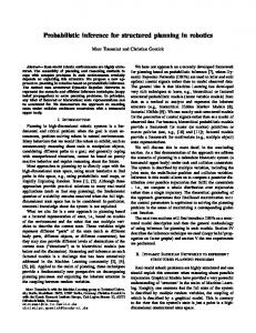
thermConditional :: (Mochastic repr, Lambda repr) => repr (HPair HReal HReal :-> HMeasure (HPair HProb HProb)) thermConditional = disintegrate thermometer Hakaru’s pretty-printer, used on thermConditional, produces Figure 2. Of course, this expression is different from thermometer. The measurements m1 and m2, which used to be drawn from normals, are now the input variables x2 and x3 (bound by deconstructing the argument x1 using unpair). In place of the two measurement calls to normal, the distribution is now weighted by the density of each Gaussian at the corresponding measurement. Unlike a distribution, a density is a function from HReal to HProb. lam $ \x1 -> x1 `unpair` \x2 x3 -> uniform 3 8 `bind` \x4 -> normal 21 (unsafeProb x4) `bind` \x5 -> uniform 1 4 `bind` \x6 -> normal x5 (unsafeProb x4) `bind` \x7 -> weight (exp_ (-(x3 - x7) * (x3 - x7) / fromProb (2 * pow_ (unsafeProb x6) 2)) / unsafeProb x6 / sqrt_ (2 * pi_)) $ weight (exp_ (-(x2 - x5) * (x2 - x5) / fromProb (2 * pow_ (unsafeProb x6) 2)) / unsafeProb x6 / sqrt_ (2 * pi_)) $ dirac (pair (unsafeProb x4) (unsafeProb x6))

Fig. 2: The thermometer model after disintegration The reader might wonder why Figure 1 is rather large, given the simple model it came from, while Figure 2 is modest though the model it comes from seems more complex. This is because the burglar model contains discrete choices (calls to bern), which tend to inflate the output of disintegration, while the thermometer model is a straight-line program. While thermConditional represents the correct posterior distribution, it is not yet efficient for inference. This is because of the two calls to normal that still exist. Our prior distribution thermometer does not return the variables drawn from these normals, which are the temperatures t1 and t2. The measure is a marginal distribution on only m1, m2, noiseT, and noiseM. Similarly, thermConditional, when given measurements, returns a distribution only on the noises, not on the variables x5 and x7. Because the distribution uses the random variables x5 and x7 only internally, running it as a sampler amounts to naive numerical integration over them, which is inaccurate and slow. It would be better to integrate over x5 and x7 exactly. We can use the simplification transformation to do it: thermSimplified = simplify thermConditional The pretty-printed output of simplifying the conditional distribution is shown in Figure 3. The remaining calls to normal have disappeared and all the weight

Probabilistic inference by program transformation in Hakaru

9

factors are combined into a single formula. By removing x5 and x7 and storing the intermediate factors that are the results of integrating these variables, Hakaru has performed what is known as marginalization or variable elimination. lam $ \x1 -> weight (recip pi_ * (1/6)) $ uniform 3 8 `bind` \x2 -> uniform 1 4 `bind` \x3 -> weight (exp_ ((x2 * x2 * ((x1 `unpair` \x4 x5 -> x4) * (x1 `unpair` \x4 x5 -> x4)) * 2 + x2 * x2 * (x1 `unpair` \x4 x5 -> x4) * (x1 `unpair` \x4 x5 -> x5) * (-2) + x2 * x2 * ((x1 `unpair` \x4 x5 -> x5) * (x1 `unpair` \x4 x5 -> x5)) + x3 * x3 * ((x1 `unpair` \x4 x5 -> x4) * (x1 `unpair` \x4 x5 -> x4)) + x3 * x3 * ((x1 `unpair` \x4 x5 -> x5) * (x1 `unpair` \x4 x5 -> x5)) + x2 * x2 * (x1 `unpair` \x4 x5 -> x4) * (-42) + x3 * x3 * (x1 `unpair` \x4 x5 -> x4) * (-42) + x3 * x3 * (x1 `unpair` \x4 x5 -> x5) * (-42) + x2 * x2 * 441 + x3 * x3 * 882) * recip (x2 * x2 * (x2 * x2) + x2 * x2 * (x3 * x3) * 3 + x3 * x3 * (x3 * x3)) * (-1/2)) * recip (sqrt_ (unsafeProb (x2 ** 4 + x2 ** 2 * x3 ** 2 * 3 + x3 ** 4))) * 3) $ dirac (pair (unsafeProb x2) (unsafeProb x3))

Fig. 3: The result of simplifying thermConditional Once again, simplification subsumes exact inference with help from computer algebra. While this code could be made yet more concise by let-binding, it already makes for an efficient sampler. 3.3

Sampling

The next step in the workflow of a Hakaru user is to sample from the posterior. In this example, the posterior distribution is only 2-dimensional, so it is easy to tune the noise parameters by importance sampling or by searching a grid exhaustively. In higher dimensions, most parameter combinations are very bad, and exhaustive search is intractable, so we often want to use a Markov chain Monte Carlo (MCMC) technique in order to get an answer in a reasonable amount of time. That is what we demonstrate here. MCMC means that the sampler generates not a single random sample but a chain of them, each dependent on the previous one. Most MCMC algorithms require specifying an easy-to-sample proposal distribution that depends on the current element of the chain [7]. This distribution is sampled to propose a candidate for the next element in the chain. We show here the Metropolis–Hastings method (MH), a popular MCMC algorithm that compares the posterior and proposal densities at the current and proposed elements in order to decide whether

10

Narayanan, Carette, Romano, Shan, Zinkov

the next element of the chain should be the proposed element or a repetition of the current element. This decision mathematically ensures that the chain is composed of samples that represent the posterior accurately. A good proposal distribution will propose samples that are representative of the posterior. In this sense, the proposal embodies a strategy for searching and approximating the posterior space. Hakaru lets us specify our own proposal distribution based on our understanding of the model. MH practitioners know that custom proposal distributions are an important way to improve MH performance. Here we show a proposal distribution that a Hakaru user could write for the current example. proposal :: (Mochastic repr) => repr (HPair HReal HReal) -> repr (HPair HProb HProb) -> repr (HMeasure (HPair HProb HProb)) proposal _m1m2 ntne = unpair ntne $ \noiseTOld noiseEOld -> superpose [(1/2, uniform 3 8 `bind` \noiseT' -> dirac (pair (unsafeProb noiseT') noiseEOld)), (1/2, uniform 1 4 `bind` \noiseE' -> dirac (pair noiseTOld (unsafeProb noiseE')))]

This particular proposal distribution leaves one noise parameter unchanged and draws an update to the other noise parameter from a uniform distribution. Thus, once the Metropolis–Hastings sampler finds a good setting for one parameter, it can remember it and more or less leave it alone for a while as it fiddles with the other parameter. In contrast, importance sampling tries to hit upon good settings for both parameters at once, which is less likely to happen. On the other hand, the chain dependency of Metropolis–Hastings sampling means it can stay stuck in a globally sub-optimal part of the search space for a long time. A generic MH algorithm can be defined as a reusable transformation on Hakaru terms. It has this type: mh

:: (Mochastic repr, Integrate repr, Lambda repr, env ~ Expect' env, a ~ Expect' a, Backward a a) => (forall r'. (Mochastic r') => r' env -> r' a -> r' (HMeasure a)) -> (forall r'. (Mochastic r') => r' env -> r' (HMeasure a)) -> repr (env :-> (a :-> HMeasure (HPair a HProb)))

The various constraints in the type are a consequence of the finally tagless embedding. The Expect, Integrate and Lambda constraints require the interpretation (repr) to define operations for expectation, integration, and the lambda calculus. The Backward constraint is required for the density calculation step that forms a part of the MH procedure. The sampling interpretation satisfies these constraints.

Probabilistic inference by program transformation in Hakaru

11

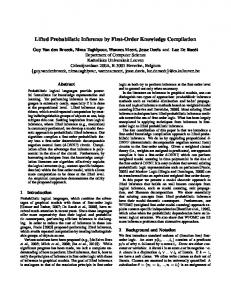
We cam apply the generic mh to our custom proposal and the desired posterior thermSimplified: mhKernel = mh proposal thermSimplified This invocation generates a Metropolis–Hastings transition kernel that can be used to produce samples from the posterior. We first condition the kernel on observed temperature measurements – pair 29 26. We then run this sampler for 20000 iterations and use every 5th sample (a process known as thinning) to produce the plot in Figure 4. noiseT 8 7 6 5 4

Value

3 0

1000

2000 noiseE

3000

4000

4

noiseT 3

0.20 2

0.15

1 0

0.10 2000

1000

3000

Sample number

4000

0.05

Density

(a) Traceplot of sampled parameter values given observed temperatures (29◦ C,26◦ C) noiseT

0.20

0.00

3

4

5

6

7

8

noiseE

0.3

0.15

0.2 0.10

0.1

Density

0.05

0.00

0.0 3

4

5

6

7

8

noiseE

1

2

Value

3

4

(b) Density plots for the noise parameters 0.3

0.2

Fig. 4: Sampling from the conditioned posterior using Metropolis–Hastings

0.1

Knowing that the MH kernel likely contains large mathematical expressions from density calculation, and knowing that the simplify transformation is modValuecan attempt to speed up the computation at each iteration ular and reusable, we of the MH kernel by invoking simplify mhKernel. The performance gained from this reuse of algebraic simplification is shown in the middle row of Table 1. Simplification here introduces efficiency with respect to wall clock time and not in the number of samples needed for convergence. The third program in Table 1 is a hand-coded Hakaru sampler written non-compositionally. For comparison, we also wrote a model of thermometer in the probabilistic language 0.0

1

2

3

4

12

Narayanan, Carette, Romano, Shan, Zinkov Source of Hakaru code

Average run time

Generated by disintegrator 2,015 ± 4ms Generated, then automatically simplified 569 ± 4 Written by hand 529 ± 10

Table 1: Time needed to draw 20,000 MH samples averaged over 10 runs.

WebPPL [5]; it generates a Metropolis-Hastings sampler that takes 948 ± 8ms. All measurements were produced on a quad-core Intel i5-2540M processor running 64-bit Ubuntu 14.04. Hakaru’s samplers use GHC 7.8.3 -O2, and WebPPL’s sampler is compiled to JavaScript and run on Node.js version 0.10.28.

4

Inference by composable program transformations

As the examples above show, Hakaru transforms a probabilistic program to other programs in the same language that generate samples or otherwise perform inference. This major design decision contrasts with most other probabilistic programming systems, which handle a probabilistic program either by producing code in a different language, or by generating samples or otherwise performing inference directly—without staging. Because Hakaru transformations stay in the same language, we can compose them. For example, we use disintegration and simplification together to generate efficient densities, which are at the heart of Metropolis–Hastings sampling, as well as conditional distributions, which are at the heart of Gibbs sampling. Even after we apply an approximate inference technique such as Metropolis–Hastings to a problem, we can still inspect and optimize the generated solution before running it. We can also compose inference techniques (such as particle filtering and Metropolis–Hastings) as well as analyses (perhaps to estimate the running time or accuracy of a sampler). 4.1

Semantic specifications of transformations

Although all our transformations operate on Hakaru syntax, we specify what they do by referring to Hakaru semantics based on integrators. For example, for the models in Section 2 and Section 3, the specification of disintegration guarantees that the denotations of the model and the posterior are related as below. model = superpose [(1, dirac true), (1, dirac false)] `bind` \alarm -> app (disintegrate model) alarm `bind` \burglary -> dirac (pair alarm burglary)

thermometer = lebesgue `bind` \m1 -> lebesgue `bind` \m2 -> app (disintegrate thermometer) (pair m1 m2) `bind` \noise -> dirac (pair (pair m1 m2) noise)

We describe elsewhere the implementation of this specification, which involves reordering integrals and computing a change of variables [12].

Probabilistic inference by program transformation in Hakaru

13

The specification of simplification is just that its output has the same measure semantics as the input. Implementing the specification involves translating to and from an integrator representation of measures, and improving the integral using computer algebra. We describe this process in detail elsewhere [2]. 4.2

Comparison with other embeddings

´ Like us, Kiselyov and Shan [6] and Scibior et al. [11] both embed a probabilistic language in a general-purpose functional language, respectively OCaml and Haskell. Like us, they both express and compose inference techniques as transformations that produce programs in the same language. But unlike our embedding, their embeddings are “shallower”: the language defines a handful of constructs for manipulating distributions, and reuses the host languages’ primitives for all other expressions. On one hand, their transformations consequently cannot inspect most of the input source code, notably deterministic computations and the right-hand side of >>=. Thus, Hakaru can compute densities and conditional distributions in the face of deterministic dependencies, and Hakaru can generate Metropolis–Hastings samplers using a variety of proposal distributions. On the other hand, a shallow embedding ensures that any deterministic part of a probabilistic program runs at the full speed of the host language. WebPPL is a probabilistic language embedded in Javascript, providing inference methods to transform input programs into a different language [5]. Venture [8] and Anglican [13] are probabilistic programming systems that build upon Lisp and Clojure respectively to define strict, impure languages for composing inference procedures. In all these works, the code – derived via transformations or building blocks – can perform direct inference but not stage any computation.

5

Expressing semantic distinctions by types

We make crucial use of types to capture semantic distinctions in Hakaru. These distinctions show up both in the implementation and in the language itself. Figure 6 illustrates the types of each construct or macro described in this paper, grouped by the interface (such as Mochastic) that an interpretation (such as Sample) would need to implement. 5.1

Distinguishing Hakaru from Haskell

The foremost distinction is between Hakaru’s type system and Haskell’s type system. That is, we distinguish between the universe 3 of Hakaru types, Hakaru, and the universe of Haskell types, *. At first this distinction may seem unnecessary, since we can identify Hakaru types as those which are the argument to some repr. However, making the distinction eliminates two broad classes of bugs. 3

We implement this universe of types by defining our own Haskell kind using GHC’s -XDataKinds extension. Thus, we call Hakaru and * both “universes” and “kinds”.

14

Narayanan, Carette, Romano, Shan, Zinkov

class (...) => Base (repr :: Hakaru * -> *) where pair :: repr a -> repr b -> repr (HPair a b) unpair :: repr (HPair a b) -> (repr a -> repr b -> repr c) -> repr c true, false :: repr HBool if_ :: repr HBool -> repr c -> repr c -> repr c unsafeProb :: repr HReal -> repr HProb fromProb :: repr HProb -> repr HReal exp_ :: repr HReal -> repr HProb pow_ :: repr HProb -> repr HReal -> repr HProb sqrt_ :: repr HProb -> repr HProb class (Base repr) => Mochastic (repr :: Hakaru * -> *) where dirac :: repr a -> repr (HMeasure a) bind :: repr (HMeasure a) -> (repr a -> repr (HMeasure b)) -> repr (HMeasure b) superpose :: [(repr HProb, repr (HMeasure a))] -> repr (HMeasure a) uniform :: repr HReal -> repr HReal -> repr (HMeasure HReal) normal :: repr HReal -> repr HProb -> repr (HMeasure HReal) class Lambda (repr :: Hakaru * -> *) where lam :: (repr a -> repr b) -> repr (a :-> b) app :: repr (a :-> b) -> repr a -> repr b bern :: (Mochastic repr) => repr HProb -> repr (HMeasure HBool) weight :: (Mochastic repr) => repr HProb -> repr (HMeasure w) -> repr (HMeasure w) liftM :: (Mochastic repr) => (repr a -> repr b) -> repr (HMeasure a) -> repr (HMeasure b)

Fig. 6: The types of language constructs and macros used in the examples

First, there are many types in * which we do not want to allow within Hakaru. For example, Hakaru has support for arbitrary user-defined regular recursive polynomial data types. However, Haskell’s data types are far richer, including: non-regular recursive types, non-strictly-positive recursive types, exponential types, higher-rank polymorphism, GADTs, and so on. Consequently, we must not allow users to embed arbitrary Haskell data types into Hakaru. The kind * is much too large for Hakaru, so by introducing the Hakaru kind we can statically prohibit all these non-Hakaru types. Second, distinguishing between Hakaru and * guarantees a form of hygiene in the implementation. Without the kind distinction it is easy to accidentally equivocate between Haskell’s types and Hakaru’s types. This equivocation introduces confusion about what exists within the Hakaru language itself, versus what exists within the interpretation of Hakaru programs. One example of this confusion is the lub operator used by disintegration to make a nondeterministic choice between two Hakaru programs that mean the same measure. When introducing the Hakaru kind we noticed that it was not entirely clear whether the lub operator is in the language or a mere implementation detail. 5.2

Distinguishing values and distributions

Hakaru’s type system draws a hard distinction between individual values (of type a) and distributions on values (of type HMeasure a). To see why this is necessary, consider the pseudo-program “x = uniform 0 1; x + x”. As written

Probabilistic inference by program transformation in Hakaru

15

it is unclear what this pseudo-program should actually mean. On one hand, it could mean that the value x is drawn from the distribution uniform 0 1, and then this fixed value is added to itself. On the other hand, it could mean that x is defined to be the distribution uniform 0 1, and then we draw two samples from this distribution and add them together. To distinguish these two meanings, stochastic languages like Church [4] must introduce a memoization operator; however, it is often difficult to intuitively determine where to use the memoization operator to obtain the desired behavior. In contrast, Hakaru distinguishes these meanings by distinguishing between letbinding and monadic-binding: sampleOnce = uniform 0 1 `bind` \x -> dirac (x + x) sampleTwice = uniform 0 1 `let_` \x -> liftM2 (+) x x Importantly, there is no way to mix up the second lines of these programs. If x is monadically bound, and hence has type HReal, then the expression liftM2 (+) x x does not type check, because HReal is not a monad so it cannot be the type of arguments to liftM2 (+). Whereas, if x is let-bound, and hence has type HMeasure HReal, then the expression dirac (x + x) does not type check, because we do not define (+) on measures; but even if we did define (+) on measures, then the expression would have type HMeasure (HMeasure HReal) which doesn’t match the signature. 5.3

Distinguishing values in different domains

It is often helpful to distinguish between various numeric domains. Although the integers can be thought of as real numbers, it is often helpful to specify when we really mean integers. Similarly, although the natural numbers can be thought of as integers and the positive reals can be thought of as reals, it is often helpful to explicitly capture the restriction to non-negative numbers. Thus, Hakaru provides four primitive numeric types: HNat, HInt, HProb, and HReal. There are at least four reasons for making these distinctions. First, it helps with human understanding to say what we mean. Second, many of the built-in distributions are only defined for non-negative parameters, thus the non-negative types HNat and HProb are necessary to avoid undefinedness. Third, capturing the integral and non-negative constraints helps with algebraic simplification since we do not have to worry about the non-occurring cases. Fourth, for the situations where we must actually compute values (e.g., the sampling interpretation), knowing that HProb is non-negative means that we can represent these values in the log-domain in order to avoid problems with underflowing. 5.4

Distinguishing different interpretations of Hakaru

We use a “finally tagless” embedding of Hakaru in Haskell [1]. Thus an interpretation of Mochastic is implemented as an instance. We have several such interpretations—a sampler, a pretty-printer, and two variants of embedding our

16

Narayanan, Carette, Romano, Shan, Zinkov

language into Maple. Transformations are also instances, but where repr appears as a free variable. For example, we have an expectation transformation Expect, which takes a measure expression and returns its expectation functional. Another transformation implements disintegration, which is performed by lazy partial evaluation of measure terms. As our use of bind indicates, we use Higher Order Abstract Syntax (HOAS) to encode Hakaru binding. In exchange for preventing scope extrusion, HOAS makes some manipulations of bindings difficult to express. Basically, one significant advantage of finally tagless is that if we can write your transformation compositionally, then it will compose beautifully with other such transformations. But some transformations are hard to write compositionally. For example, it is easy to write “macros” such as liftM2, as well as the Expect transformation, but it is hard to implement lazy partial evaluation. Even for a compositional transformation, finally-tagless style makes our code hard to debug, because for example Expect repr is implemented in terms of an abstract repr that is not required to be an instance of Show. This rules out using Debug.Trace.traceShow in the middle of the implementation of Expect. We love how the Haskell type of a Hakaru term tracks how the term will be interpreted, such as Expect PrettyPrint. The flip side is that to apply multiple interpretations to the same term (like to scale a distribution so it sums to 1), we must either create the “product” of two interpretations (and using it to interpret a term takes time exponential in the number of nested binders in the term), or the Haskell type of a term must be universally quantified over repr. The latter is very natural for experienced Haskell programmers, but is hard to explain to others, thus limiting the potential of Hakaru as a general-purpose probabilistic programming language. Another issue is that the very hygiene which is a strength of finally-tagless makes it awkward to have “free variables” (parameters) in a term; these must all be lam bound before a term can be disintegrated or simplified. This contrasts sharply with how easily a computer algebra system handles free variables in equivalent terms [2].

6

Conclusion

A major challenge faced by every probabilistic programming system is that probabilistic models and inference algorithms do not compose in tandem: just because a model we’re interested in can be built naturally from two submodels does not mean a good inference algorithm for the model can be built naturally from good inference algorithms for the two submodels. Due to this challenge, many systems with good support for model composition resort to a fixed or monolithic inference algorithm and do their best to optimize it. Hakaru demonstrates a new way to address this challenge. On one hand, Hakaru supports model composition like any other embedded monadic DSL does: on top of primitive combinators such as dirac, bind, and superpose, users can define Haskell functions to express common patterns of samplers and measures. On the other hand, because each inference building block is a transformation on

Probabilistic inference by program transformation in Hakaru

17

this DSL, Hakaru supports inference composition like a compiler construction kit or computer algebra system does: users can define Haskell functions to express custom pathways from models to inference. We are working to extend the Hakaru language, to express high-dimensional models involving arrays and trees, and to express more inference algorithms, including parallel and streaming ones. We are also working to make Hakaru more usable: by representing the abstract syntax as a data type, by customizing the concrete syntax, and by inviting user interaction for transforming subexpressions.

References [1] Carette, J., Kiselyov, O., Shan, C.c.: Finally tagless, partially evaluated: Tagless staged interpreters for simpler typed languages. Journal of Functional Programming 19(5), 509–543 (2009) [2] Carette, J., Shan, C.c.: Simplifying probabilistic programs using computer algebra (2015), http://www.cs.indiana.edu/ftp/techreports/TR719.pdf [3] Giry, M.: A categorical approach to probability theory. In: Banaschewski, B. (ed.) Categorical Aspects of Topology and Analysis: Proceedings of an International Conference. pp. 68–85. Springer (1982) [4] Goodman, N.D., Mansinghka, V.K., Roy, D., Bonawitz, K., Tenenbaum, J.B.: Church: A language for generative models. In: Proceedings of the 24th Conference on Uncertainty in Artificial Intelligence. pp. 220–229. AUAI Press (2008) [5] Goodman, N.D., Stuhlm¨ uller, A.: The design and implementation of probabilistic programming languages. http://dippl.org (2014), accessed: 2015-11-20 [6] Kiselyov, O., Shan, C.c.: Embedded probabilistic programming. In: Proceedings of the Working Conference on Domain-Specific Languages. pp. 360–384. No. 5658 in Lecture Notes in Computer Science, Springer (2009) [7] MacKay, D.J.C.: Introduction to Monte Carlo methods. In: Jordan, M.I. (ed.) Learning and Inference in Graphical Models. Kluwer (1998) [8] Mansinghka, V.K., Selsam, D., Perov, Y.N.: Venture: a higher-order probabilistic programming platform with programmable inference. CoRR abs/1404.0099 (2014), http://arxiv.org/abs/1404.0099 [9] Pearl, J.: Probabilistic Reasoning in Intelligent Systems: Networks of Plausible Inference. Morgan Kaufmann (1988), revised 2nd printing, 1998 [10] Ramsey, N., Pfeffer, A.: Stochastic lambda calculus and monads of probability distributions. In: POPL ’02: Conference Record of the Annual ACM Symposium on Principles of Programming Languages. pp. 154–165. ACM Press (2002) ´ [11] Scibior, A., Ghahramani, Z., Gordon, A.D.: Practical probabilistic programming with monads. In: Proceedings of the 8th ACM SIGPLAN Symposium on Haskell. pp. 165–176. ACM Press (2015) [12] Shan, C.c., Ramsey, N.: Symbolic Bayesian inference by lazy partial evaluation (2015), http://www.cs.tufts.edu/~nr/pubs/disintegrator-abstract.html [13] Wood, F., van de Meent, J.W., Mansinghka, V.: A new approach to probabilistic programming inference. In: Proceedings of the 17th International conference on Artificial Intelligence and Statistics. pp. 1024–1032 (2014)