Probabilistic Modeling of Duration of Load Effects in ...

Presented at the 35. CIB W18 Meeting in Kyoto, September 2002

Probabilistic Modeling of Duration of Load Effects in Timber Structures Jochen Köhler Swiss Federal Institute of Technology ETH, Switzerland Staffan Svensson Dept. Building Technology and Structural Engineering, Aalborg University, Denmark Keywords: Timber, Reliability, Duration of Load (DOL), Damage Accumulation, Creep Rupture, Damaged Viscoelastic Material Theory, Load Processes.

Abstract: Reliability analysis of structures for the purpose of code calibration or reliability verification of specific structures requires that the relevant failure modes are represented and analyzed. For structural timber, sustaining a lifelike load, two failure cases for each failure mode have to be considered. These two cases are: maximum load level exceeding load-carrying capacity, and damage accumulation (caused by the load and its duration) leading to failure. The effect of both load intensity and load duration on the capacity of timber has been an area of large interest over the last decades. Several research projects address this problem and a number of different damage models, based on experimental evidence, have been formulated to describe the phenomenon. Three damage models are analyzed in this study. In the present paper a method for probabilistically modeling the effect of load duration is presented. The method accounts for the overall imprecision of the damage models in comparison to experiments, the variability of the damage models parameters, and the dependency between the parameters. The method is consistent in such a way that it includes the damage models themselves as well as the accuracy in relation to actual data. This allows the calculated long-term behavior of the structure to be directly connected to the experimental data on which the damage model is calibrated. This is shown in simulations applying three different well-known damage models. The DOL effect is usually taken into account in code based design of timber structures in terms of a modification factor kmod which is multiplied on the short term resistance of the timber material. The scenario of a beam subject to office space life loads is analyzed and the modification factor kmod is calibrated for each damage model.

Presented at the 35. CIB W18 Meeting in Kyoto, September 2002

Introduction The load-carrying capacity of timber is significantly reduced under sustained load. This effect of load duration (DOL) is well known for timber. The general hypothesis is that load duration creates damage in the timber material at load levels below load levels leading to failure in short-term tests. If the accumulation of damage, caused by the duration of load, continues, it will with time lead to failure. For a timber structure sustaining a load with constant intensity the observed failure is referred to a creep rupture failure. For timber structures sustaining a lifelike load for which the intensity varies with time the failure is not given to be a creep rupture failure. Research on both clear wood (e.g. Wood 1947,1951) and structural timber (e.g. Madsen 1974 and Hoffmeyer 1990) sustaining long-term constant load is documented in the literature. From existing experimental data it is possible to obtain a reasonable estimate of the reduction of loadcarrying capacity, as a function of time under constant load. In practice, however, load excitation on structures fluctuates significantly and is not constant in time. For a normal case of time-variable load, reduction of load-carrying capacity of structural timber must be estimated by other means. Three damage theories widely spread in the field of DOLresearch and investigated in this study are Gerhards’ model (Gerhards 1977, 1979 and Gerhards and Link 1987), Foschi and Yaos’ model (Foschi and Yao 1986) and Nielsens’ model (Nielsen 1979 and in Madsen 1992). It should be underlined that most models estimating DOL-effects are originally founded on the case of constant load and estimate the effect of DOL in relation to the assumed short-term load-carrying capacity. The models are, however, utilized for cases with time-varying load levels. In timber design codes, effects of load duration are accounted for by a strength modification factor, kmod, which depends on the type of load acting on the structure. The loads are classified in terms of their expected duration time and intensity. Calibration of kmod, accounting for DOL by applying damage theories in probabilistic analyses, has been carried out and reported by Foschi et al. (1989), Ellingwood et al. (1991), Svensson et al. (1999), and Sorensen et al. (2002). Different approaches to describe with time decreasing capacity for the prevailing load and the load history have been used. In the following, a method to calibrate kmod by also including the applied damage model uncertainty to represent experimental data is presented. With this method the outcome of the kmod calibration is directly connected to the accuracy of the damage model to represent experimental data.

Live load model The live load model used in this study is the model proposed in (CIB 1989) and recommended by the Joint Committee on Structural Safety (JCSS, 2001). The model contains two parts, sustained live load and intermittent live load. The sustained live load covers ordinary live load such as furniture, average utilization by persons, etc. The intermittent live load describes the exceptional load peaks, e.g. furniture assembly while re-modeling, people gathering for special occasions, etc. The live load model is based on the following definitions: The occurrences of changes in magnitude of the sustained load are modeled as a Poisson process. The duration of load will then be exponential distributed with expected value λsus.

2

Presented at the 35. CIB W18 Meeting in Kyoto, September 2002

The magnitude of the sustained load is modeled by a Gamma distribution with expected A0 2 2 value µsus and standard deviation σ sus = σ sus κ , r + σ sus , sp A The occurrences of intermittent loads are also modeled as a Poisson process. The duration between intermittent loads are thus exponentially distributed with expected value νint. The magnitude of the intermittent load is modeled by a Gamma distribution with expected A0 2 value µint and standard deviation σ int = σ int, κ . The duration of the intermittent load sp A tint is considered exponentially distributed. Parameters used to model live load are given in table 1. Table 1. Parameters used for model live load in office space Type of building Office

A0 m2 2

µ sus

kN/m2 0.5

σ sus,r

kN/m2 0.3

σ sus,sp 1/λsus kN/m2 0.6

year 5

µ int

kN/m2 0.2

σ int,sp

kN/m2 0.4

νint

tint

year days 0.3 1-3

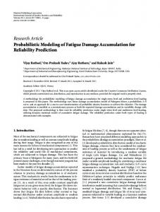
In the study, a floor structure based on joists with a span of 3.5-5.5 m and a spacing of 0.6 m is considered. The area, A, is assumed to cover the span and twice the spacing of the joists A=5m2. The peak factor, κ, is calculated for load influence on the joist for maximum mid-span bending moment, therefore κ = 1.778. In table 2 results derived when simulating the model for live load in office space are shown and in figure 1 an example of 50 years of live load is presented. Table 2. Results from simulations of live load in office space (non-parametric) Annual max mean COV kN/m2 [-] 0.96 0.78

4 3.5 3 2.5 2 1.5 1 0.5 0

50 year max mean COV kN/m2 [-] 3.05 0.29

98% quantile kN/m2 3.10

Load

0

10

20

30

Time [year] 40 50

Figure 1. A typical live load realization acting as midspan bending moment on a joist beam in an office space.

3

Presented at the 35. CIB W18 Meeting in Kyoto, September 2002

Load-carrying capacity model Initial load-carrying capacity Initial load-carrying capacity of structural timber, R0, is determined by loading an undamaged structural timber member with a ramp load with constant loading rate k until failure. The rate of loading and the test procedure have to be in accordance with the prevailing code. This capacity is frequently referred to as the short-term capacity. The strength of the structural timber is then defined for that particular mode of testing. If bending moment capacity is tested, the bending strength, fm, of the structural member is the capacity divided by the resistance moment as a geometric quantity. For known bending strength the initial capacity is here determined as:

R0 = fm a where a is the geometric quantity.

Damage models Three different damage models are investigated in this study. They are named after their developers as Gerhards’ model (Gerhards 1977, 1979 and Gerhards and Link 1987), Foschi and Yaos’ model (Foschi and Yao 1986), and Nielsens’ model (Nielsen 1979 and in Madsen 1992). The two first models are usually described as phenomenological models and the latter is a fracture mechanics based model. The models are all functions of the initial short-term capacity, as defined above. This makes calibration and verification of the models against duration of load tests unambiguous, since the initial capacity of a sample failed in long-term load case is hypothetical. In the calibration of the models shown later the (assumption) equal rank sampling (Madsen 1992) is utilized for estimating the initial strength of sample failed in duration of load tests. In the following the mathematical expressions for each model is presented. The models were originally presented in a stress – strength perspective the small modification of using a load effect – load capacity perspective has here been done.

Gerhards’ model Equation (1) shows the mathematical expression of Gerhards’ model for calculating damage accumulation of a timber member with initial capacity, R0, sustaining a load, S(t). The degree of damage, α, is defined in the range α = 0 denoting no damage and α =1 denoting failure. a and b are model parameters. S (t )

− a +b dα R0 =e dt

for 0 ≤ α ≤ 1

(1)

By solving equation (1) for the case of determining the short-term capacity R0, with a standard test procedure as previously described, one will ascertain the following expression for the model parameter a:

4

Presented at the 35. CIB W18 Meeting in Kyoto, September 2002

a = ln(

R0 b (e − 1)) bk

(2)

where k is the rate of loading dS(t)/dt. The damage caused by a period of constant load level, Ŝ, when derived from equation (1) is: Sˆ   b  bk e R 0  t + α 0 α (t ) =  b  R0 (e − 1)   

for 0 < α 0 < α (t ) ≤ 1

(3)

where α0 is the degree of damage prior to the studied period of constant load. Time to failure, tf, for a prior-to-testing undamaged member loaded with a ramp load, with the same rate of loading, k, as the standard test, to the constant load level, Ŝ, is reached and held until failure occurs has the following expression: Sˆ Sˆ R0  b (1− R0 )  −1 tf = + e  k kb   

for

Sˆ < R0

(4)

Equation (4) is used here when calibrating the model against test results.

Foschi and Yao Model Equation (5) shows the mathematical expression of Foschi and Yao’s model for calculating damage accumulation of a timber member with initial capacity, R0, sustaining a load S(t). The degree of damage, α, is also in this model defined in the range α = 0 denoting no damage and α =1 denoting failure. B

D

 S (t )   S (t )  dα = A − η  + C  − η  α (t ) dt  R0   R0  dα =0 dt

for

S (t ) > ηR0 (5)

for S (t ) ≤ ηR0

A, B, C, and D are model parameters. With the model expressed as equation (5) the model parameters C and D are dimensionless and A and B have the dimension time-1. This is a modification of the original proposal by Foschi and Yao, however, the model is not compromised by this modification. η is the threshold ratio and, as expressed in equation (5), no damage will accumulate for load effects below the threshold level, which is defined as the product of initial capacity and threshold ratio. There is no evidence of structural timber healing, which means that the threshold is constrained between zero and unity, the latter bound referring to material not affected by DOL.

5

Presented at the 35. CIB W18 Meeting in Kyoto, September 2002

By solving equation (5) for the case of determining the short-term capacity R0, with a standard test procedure as previously described, one will ascertain also for Foschi and Yaos’ model one model parameter, A, with the equation: A=

k ( B + 1) R0 (1 − η ) ( B +1)

(6)

where k is the rate of loading dS(t)/dt. The damage caused by a period of constant load level, Ŝ, when derived from equation (5) is:

α (t ) = κα 0 + κλ − λ α (t ) = 0

Sˆ > ηR0 , Sˆ < R0 , 0 < α 0 < α (t ) ≤ 1 Sˆ ≤ ηR 0

(7)

κ =e λ=

Sˆ C ( −η ) D ∆t R0

k ( B + 1) Sˆ ( − η ) B−D ( B +1) R0 CR0 (1 − η )

where α0 is the degree of damage prior the studied period of constant load. The time to failure, tf, for a prior-to-testing undamaged member loaded with a ramp load, with the same rate of loading, k, as the standard test, until the constant load level, Ŝ, is reached and held until failure occurs has the following expression: tf =

Sˆ + k

 1+ λ   ln α 0 + λ  Sˆ  D C( − η) R0

1

tf = ∞

Sˆ > ηR0 , Sˆ < R0 (8) Sˆ < ηR0

Equation (8) is used when calibrating the model against test results.

Nielsen’s Model A model based on fracture mechanics was proposed by Nielsen (1979). The main idea behind the ‘Damaged Viscoelastic Material’ (DVM) model is that structural timber may be seen as an initially damaged viscoelastic material, with the load-carrying capacity R0 and where the damage is represented by cracks along the fibers. The time-dependent behavior of timber under load is modeled by a single crack under stress perpendicular to the crack plane. For the case of a constant load level, Ŝ, a damage accumulation law can be formulated from the DVM-model as

6

Presented at the 35. CIB W18 Meeting in Kyoto, September 2002 −

1

2 −1  b  2  Sˆ     Sˆ    dα κ (π ⋅ FL ) = α κ ⋅    α κ ⋅   (9) − 1   8q τ dt   R0     R0     FL is the strength level defined as the ratio σcr/ σl between the short-term strength, σcr, measured in a very fast ramp test and the intrinsic strength of the (hypothetical) noncracked material σl. The damage, ακ, is defined as the ratio between the actual crack length, l, and the initial crack length l0. ακ = 1 corresponds to no damage and ακ = (Ŝ/R0)-2 to full damage. τ and b are creep material parameters depending e.g. on loading mode and 1 climate history. q is given as a function of the creep exponent b as q = (0.5(b + 1)(b + 2 )) b and considers a parabolic increasing crack propagation. It should be underlined that, compared with the original DVM-model, (Ŝ/R0) replaces the ‘stress level’ SL which is defined by SL = σ / σcr where σ is the stress as a consequence of an applied load. Nielsens definition of stress level differs from the one used in this study. The time to failure tf can be expressed by the time between ακ (t = 0) = 1 and ακ (tf) = (Ŝ/R0)-2, as: 2

tf =

 π  

Sˆ  ⋅ FL ⋅  R0 

(ϕ − 1) ∫ ϕ dϕ

SL−2

8 qτ 2

1

b

(10)

1

where φ is a damage state variable. Equation (10) is used when calibrating the model against test results.

Calibration of damage models to test For the three damage models an expression for the time to failure was derived above. These expressions can be written in the general form, equation (11). This allows for the estimation of the time to failure based on the models. t f ,m = t f ,m (S R ,θ,C)

(11)

where SR is the ratio between applied load to short term strength. θ = (θ1, θ2,…, θk)T is a vector of model parameters and C = (C1, C2,…,Cj)T is a vector of constants. The estimation of the model parameters is performed in n simultaneous observations of the time to failure tf = (tf,1,tf,2,…,tf,n)T and the indicator SR = (SR,1, SR,2,.., SR,n)T. Assuming that (at least) locally the relationship between tf and SR can be described with the models, the parameter assessment may be performed by introducing an error term ε which takes account for the difference between observed time to failure tf and modeled time to failure tf,m. t f = t f , m (S R , θ, C) + ε

(12)

Assuming that the error term is normally distributed with zero mean and unknown standard deviation, σε, the maximum likelihood method, see e.g. Lindley (1965), may be used for estimating the mean values and covariance matrix for the parameters θ and σε. 7

Presented at the 35. CIB W18 Meeting in Kyoto, September 2002

The likelihood is then given as n

L(θ1 , θ 2 ,..., θ n , σ ε ) = ∏ i =1

 1  − t f ,i + t f , m ,i ( S R ,i , θ, C) 2    exp −   2 σε 2π σ ε    1

(13)

The parameters are estimated by the solution of the optimization problem (14)

max L (p) p

where p = (θ1 ,θ 2 ,...,θ n , σ ε )T . It can be shown that the estimated parameters asymptotically become normally distributed with mean values µ = p*, i.e. the parameter values satisfying equation (14). By considering instead of the likelihood function L the log-likelihood function l l = ln(L)

(15)

the covariance matrix for the parameters p = (θ1, θ2,…, θn, σ ε)T may be obtained through the inverse of the Fischer information matrix with components given by

H ij = −

∂ 2l ∂p ∂p i j

(16) p =p ∗

The parameters of the damage models are calibrated on results from long-term tests (Hoffmeyer, 1990). The considered test was performed on structural timber in four point bending. In all, 306 specimens of graded Norway spruce were tested. One third was tested in standard short-term test with ramp load until failure (prEN 408, 1994). The remaining specimens were tested with constant load corresponding to the 5 percentile for one half the sample and the 15 percentile for the other half. The tests where conducted in a constant climate corresponding to a 20% moisture content for the timber. In figure 2 the test results are presented. The abscissa in the diagram, figure 2, represents the time to failure in logarithmic hours for a beam sustaining a constant load and the ordinate represents the ratio of load and initial short-term load-carrying capacity. The matching of initial shortterm capacity for the long-term test was based on the assumption of equal rank. This assumption states that the order of failure in short-term test matches 3 to 5. For Gerhards’ damage model and Foschi and Yaos damage model the ramp rate, k, was set to 500 MPa/hour. The threshold ratio, η, in Foschi and Yaos’ model was set to a constant value of 0.5. In Nielsen’s damage model the parameters b and FL are held constant with values 0.2 and 0.25, respectively.

8

Presented at the 35. CIB W18 Meeting in Kyoto, September 2002

1

S/R0

Gerharts Nielsen

0.9

Foschi 15%-frac.

0.8

5%-frac

0.7 0.6 0.5 time [log (hours)]

0.4 -1.5

0

1.5

3

4.5

6

Figure 2. Duration of load data (Hoffmeyer, 1990) and damage models based on the mean value from an ML-estimation on the data. Table 3: Model parameters for the Foschi and Yao damage model calibrated on results form DOL tests (Hoffmeyer, 1990) by the ML-method. Model parameter D C B

σeps

Expected value 4.37 12.06 20.16 0.37

Standard deviation 0.31 7.29 0.610 0.02

With the ML method also the correlation, ρ, between the parameters is determined. For the Foschi and Yao model the following correlation was found: ρBC = 0.62, ρBD = 0.49, and ρCD = 0.97. The standard deviation of the error term σ ε is not correlated to B, C or D. Table 4: Model parameter for Nielsen’s damage model calibrated on results form DOL tests (Hoffmeyer, 1990) with the ML method. Model parameter

τ σeps

Expected value 75.74 0.38

Standard deviation 5.41 0.02

Correlation 0

Table 5: Model parameter for Gerhards’ damage model calibrated on results form DOL tests (Hoffmeyer, 1990) with the ML-method. Model parameter B

σeps

Expected value 43.35 0.476

Standard deviation 0.004 0.03

9

Correlation 0

Presented at the 35. CIB W18 Meeting in Kyoto, September 2002

Procedure of calibrating the modification factor kmod Code format The building codes, found rules of structural design in a deterministic format. In its most general form, the design equations require that a design value of the load effect, Sd, never exceeds the design value of a structural member’s load-carrying capacity, Rd. In a partial safety factor code format, the design values (in its simplest form) consist of characteristic values and partial coefficients, γ as given in equation (17). Rd = z

R0,k

γR

≥ Sk ⋅γ S = Sd

(17)

where index k denotes characteristic value and z is the design parameter. Irrespective of the duration of load, the load description (right hand-side of equation (17)) is based on the annual maximum load level, i.e. the description of load effect will not change to account for load duration. For materials being affected by load duration a modification factor, kmod, is introduced on the capacity as: Rd = z

k mod ⋅ R0,k

(18)

γR

The whole effect of load duration is accounted for by the kmod factor and the partial coefficient, γR, connected to the capacity is independent of load duration.

Probabilistic format Two failure cases (for each failure mode), load intensity exceeding the capacity, and damage accumulation during load duration leading to failure are considered. Hence, when conducting the reliability analyses each failure case is connected to a specific limit state function. For analyzing the case of load intensity, S, exceeding the initial load-carrying capacity, R0, for a reference time period the short-term limit state function in equation (19) is used. g = zR0 X R − S

(19)

where XR is the model uncertainty, normal distributed with mean equal to 1 and a COV of 5%.. For the case of damage accumulation leading to failure, αult, of a beam sustaining a load S(t) variable with time, the long-term limit state function is given in the equation below g = α ult − α (p, S (t ), z )

(20)

where α is the damage as a function of the model parameters p, S(t) is the load history, and z is the design variable. 10

Presented at the 35. CIB W18 Meeting in Kyoto, September 2002

Procedure of determining of kmod By utilizing Monte Carlo simulation for generating random variables the modification kmod has been determined according to the following procedure. The partial safety factor for the short-term strength γR,S is calibrated to a target reliability index, βt, using the limit state function (19) and the design equation (17) for constant γS. The load distribution is based on the maximum load for a reference period of 50 years. The partial safety factor for the long-term strength γR,L is calibrated using the limit state function, equation (20), and the design equation (17) for constant γS. The live load S(t) in the limit state function, equation (20), is generated based on the parameters in table 3 for the service life of 50 years. For the generated load scenario, the damage models calculate the accumulation of damage in the timber beams. Failure calculated by the three damage models is directly comparable since it is calculated on the same (identical) load scenarios. After a sufficient number of simulations, the ratio of number of failures and the total number of realizations estimates the probability of failure Pf. The corresponding reliability index is determined from β = Φ-1(pf). The long-term partial coefficient, γR.L, is re-calculated until the target reliability index, βt, is reached. kmod is then determined as: k mod =

γ M , S (β t ) γ M , L (β t )

The calculations are based on the load model given in tables 1 and 2. The values of the parameters for the damage models are given in tables 3 – 4. The short-term load-carrying capacity R0 is modeled as log-normally distributed with mean 1 and the standard deviation 20%. Referring to the Eurocode a target reliability βt = 3.8 for a reference period of 50 years is used.

Results and Discussion Three different damage models have been analyzed in this study. They have been fitted to a set of DOL data using the ML-method for estimating their parameters. In Figures 3 to 5 realizations of the models based on the ML estimated parameters for time to failure for the case of constant load (load ratio S/R0) is presented. The data are the heavy continuous curves, each calculated model value is marked as diamond marker, and the mean value of the model is the thin continuous curve. Comparison of the diagram indicates that the difference of the model when estimating time to failure for constant load is minor within the data range. A tendency of deviation between the models is, however, found in the end tail of the data range, around 4 to 5 log hours. Here the models project different paths. The Foschi and Yao model follows the data up to 4.5 log hours thereafter the model projects a path seemingly overestimating the test data. Nielsen’s model, on the other hand, projects a path that underestimates the data of the end tail. Compared to the end tail of the data Gerhards’ model shows the largest overestimation. For load ratio values above 0.9, above the data range, Nielsen’s model shows a very different behavior compared to the other models. This can be explained by the fact that Nielsen’s model, as expressed in equation (9), is restricted to load ratios below unity.

11

Presented at the 35. CIB W18 Meeting in Kyoto, September 2002

S/R 0 1 0.9 0.8 0.7 0.6 0.5

time [log hour]

0.4 -1.5

0

1.5

3

4.5

6

Figure 3. Realization of time to failure according to the Foschi and Yao model when based on the ML- estimated model parameters shown in table 3 together with the parameters correlation and the error term σeps. S/R 0 1 0.9 0.8 0.7 0.6 0.5

time [log hour]

0.4 -1.5

0

1.5

3

4.5

6

Figure 4. Realization of time to failure according to Nielsen’s model when based on the ML- estimated model parameter shown in table 4 together with the error term σeps. S/R 0 1 0.9 0.8 0.7 0.6 0.5

time [log hour]

0.4 -1.5

0

1.5

3

4.5

6

Figure 5. Realization of time to failure according to Gerahards’ model when based on the ML- estimated model parameter shown in table 5 together with the error term σeps.

12

Presented at the 35. CIB W18 Meeting in Kyoto, September 2002

When comparing, the damage models’ estimation of the time to failure for a constant load only minor differences were found. When investigating the damage accumulation for a case with constant load the models show very different behavior. In figure 6 the damage accumulation for a case of constant load (load ratio = 0.7) until failure is shown. The ordinate of the diagram in figure 6 is the difference between damage, α, and damage at failure, αf, on the abscissa is time. The damage accumulation according to Gerhards’ model is for this load case linear with time. Nielsen’s model shows for the same case high non-linearity as does Foschi and Yao’s model. The latter is, however, smoother than the first.

α -α f 1

B

0.8 A

0.6 0.4

C

0.2 0

time

Figure 6. Damage accumulation for the case of constant load ratio of 0.7 according to A) Foschi and Yao’s model B) Nielsen’s model and C) Gerhards’ model The results from the calibration of kmod factor for the case with live load in office space are shown in table 6. The results show that the damage models give almost the same result. This might not be a surprise when looking at the figures 3 to 5 in the times representing the duration of intermittent load, 1-3 days around 1.5 log hours, and the duration between intermittent loads, 1/3 of a year around 3.5 log hours where the models estimate very similar load ratios, i.e. allowable load. Table 6. Calibrated values of kmod for the different damage models. Foschi and Yao 0.77

Nielsen 0.76

Gerhards 0.75

Conducting reliability analyzes accounting for all prevailing uncertainties is of high priority, since it is the uncertainties that affect the outcome. For the studied case of longterm load additional uncertainties are introduced compared to the short-term case. Introducing models for estimating failure is one way of increasing uncertainty. If the models are dependent on a hypothetical quantity the uncertainty may be hard to quantify. This is the case for damage (according to the models studied herein) acquired during longterm load, which is dependent on an initial capacity defined in a short-term test. In addition to this the models used herein were calibrated against tests where the load level, after loading, was held constant for the whole load duration until failure. The load level for the load scenario, live load, analyzed in the reliability evaluation is, however, not 13

Presented at the 35. CIB W18 Meeting in Kyoto, September 2002

constant with time. This gives an uncertainty of higher order since there might be additional failure mechanisms for the case of with-time-variable load level that are not captured in long-term tests with constant load level. None of the above uncertainties have been accounted for in this study.

Conclusion In this paper a method for probabilistically modeling the effect of load duration is presented. The method was exemplified for calibrating the code modification factor kmod for live load in office space. Three different damage models have been applied in the method for determining the effect of load duration. The damage models were calibrated against duration of load tests using the maximum likelihood estimation as a part of the described probabilistic method. The damage models were also thoroughly investigated and compared. The following main conclusions of this study are: The Maximum likelihood method, used to determine damage model parameters for given experimental data, facilitates the advantage if accounting for parameter variation and correlation, and estimating of the overall model precision. The three damage models when realized using the parameters from the ML fit show similar characteristics for the case of time to failure of beams sustaining a constant load level, within the time range of the experimental data. If the models are extrapolated outside this range some different characteristics are observed. The damage accumulation for the case of constant load is for the damage models significantly different. Gerhard’s model shows linearity of damage accumulation with time and the others show highly non-linear behavior. When calibrating kmod-factor for the case of live load in office space the different damage models give similar values.

Acknowledgements The experimental test results used in this study were provided to us by Dr P Hoffmeyer and his contribution made this research possible. The work described in the present paper was conducted as part of the European research project, Reliability design of timber structures’ under the EC Action COST E24. The financial support from the Federal Office of Education and Science, Switzerland is gratefully acknowledged.

References BARRETT, J.D., FOSCHI, R.O., 1978. ‘Duration of load and probability of failure in wood.’ Part I + II, Canadian Journal of Civil Engineering, 5(4):505-532. ELLINGWOOD, B.,ROSOWSKI, D. V., 1991. ‘Duration of Load effects in LRFD for wood constructions.’ ASCE J. Struct. Eng. 117(2):584-599.

14

Presented at the 35. CIB W18 Meeting in Kyoto, September 2002

CIB Commision W81. (1989). Actions on Structures – Liveloads in Buildings. CIB Publication 116 FOSCHI, R.O., YAO, Z.C., 1986. ‘Another look at three duration of load models.’ Proc. 19th CIB/W18 Meeting, Florence, Italy. GERHARDS, C.C., 1979. ‘Time-related effects of loads of wood strength. A linear cumulative damage theory.’ Wood science, 19(2):139-144. GERHARDS, CC., LINK, C.L., 1987. ‘A cumulative damage model to predict load duration characteristics in lumber.’ Wood and Fiber Science, 19(2):147-164. HOFFMEYER, P., 1990. ‘Failure of Wood as Influenced by Moisture and Duration of Load.’ PhD Thesis, College of Environmental Science and Forestry Syracuse, State University of New York. Joint Committee on Structural Safety 2001. ‘Probabilistic Model Code’, Internet Publication: www.jcss.ethz.ch. LINDLEY, D. V. ,1965. ‘Introduction to Probability & Statistics’ Cambridge University Press. MADSEN, B. ,1992. ‘Structural Behavior of Timber’. Timber Engineering Ltd., Vancouver, Canada. NIELSEN, L.F., 1979. ‘Crack failure of dead-, ramp- and combined loaded viscoelastic materials.’ Proceedings First International Conference on Wood Fracture, Banff, Alberta, Canada. NIELSEN, L.F., 2000. ‘Lifetime and Residual Strength of wood subjected to static and variable load – Part I +II.’, Holz als Roh- und Werkstoff 58: 81-90 and 141-152. Springer,. SORENSEN, J.D., STANG, B.D., SVENSSON, S., 2002 ‘Calibration of duration factor kmod.(draft)’ to be published. FOSCHI, R.O., FOLZ, B.R., AND YAO, F.Z., 1989. ‘Reliability-based Design of Wood Structures’. Structural Research Series, Report No. 34, Department of Civil Engineering, University of British Columbia, Vancouver, British Columbia, Canada. SVENSSON, S., S. THELANDERSSON AND H. J. LARSEN, 1999. ‘Reliability of timber structures under long term loads’. Materials and structures, Vol. 32, pp 755760.

15