Article
Probabilistic Multi-Sensor Fusion Based Indoor Positioning System on a Mobile Device Xiang He, Daniel N. Aloi and Jia Li * Received: 16 September 2015; Accepted: 9 December 2015; Published: 14 December 2015 Academic Editor: Leonhard M. Reindl Department of Electrical and Computer Engineering, Oakland University, 2200 N Squirrel Road, Rochester, MI 48309, USA;
[email protected] (X.H.);
[email protected] (D.A.) * Correspondence:
[email protected]; Tel.: +1-313-205-7274
Abstract: Nowadays, smart mobile devices include more and more sensors on board, such as motion sensors (accelerometer, gyroscope, magnetometer), wireless signal strength indicators (WiFi, Bluetooth, Zigbee), and visual sensors (LiDAR, camera). People have developed various indoor positioning techniques based on these sensors. In this paper, the probabilistic fusion of multiple sensors is investigated in a hidden Markov model (HMM) framework for mobile-device user-positioning. We propose a graph structure to store the model constructed by multiple sensors during the offline training phase, and a multimodal particle filter to seamlessly fuse the information during the online tracking phase. Based on our algorithm, we develop an indoor positioning system on the iOS platform. The experiments carried out in a typical indoor environment have shown promising results for our proposed algorithm and system design. Keywords: indoor positioning; HMM framework; graph structure; multimodal particle filter; sensor fusion; iOS platform
1. Introduction In recent years, researchers have developed various approaches for mobile-device (smartphone, tablet) user-positioning in GPS-denied indoor environment. To name a few, radio frequency (RF) fingerprinting techniques, motion-sensor-based pedestrian dead reckoning (PDR) techniques, and visual-sensor-based feature matching techniques, are some of the most popular approaches in indoor positioning. However, all of them have their own limitations. RF fingerprinting techniques (Bluetooth [1], RFID [2], Zigbee [3] and WiFi [4–6],) have the problem of signal fluctuation due to the multipath fading effect in indoor environment. The motion-sensor-based PDR approach [7,8] suffers from the fact that the motion sensors equipped in the mobile device are low cost Micro Electromechanical System (MEMS) sensors, which have relatively low accuracy. Thus, the integration drift will cause the positioning error to accumulate over time. The visual-sensor-based positioning techniques [9–13] extract features (SIFT [14], SURF [15]) from captured images and compare them with an image database. These techniques are limited by their costly feature-matching algorithm and restricted computation resources on a mobile platform. In ASSIST [16], acoustic signals emitted from smartphone speakers are adopted to locate the user using the time difference of arrival (TDoA) multilateration method. ASSIST can locate the user within 30 cm. However, this method requires sound receivers to be preinstalled in ceilings or walls, which adds extra infrastructure to the indoor environment. To overcome the drawback of each sensor, people have come up with fusion approaches to combine different sensors to achieve a better positioning result. However, since the sensors are measuring different physical phenomena, it is not an easy task to effectively fuse the information
Sensors 2015, 15, 31464–31481; doi:10.3390/s151229867
www.mdpi.com/journal/sensors
Sensors 2015, 15, 31464–31481
from multiple sensors. The existing sensor fusion approaches for positioning involve decision-level fusion and feature-level fusion. Decision-level fusion usually contains multiple local detectors and a fusion center. The local decisions are transmitted to the fusion center where the global decision is derived. The optimum decision rule under the Neyman-Pearson sense can be expressed as a function of the correlation coefficients of the local detectors. It has been shown that the performance of such distributed detection systems degrade as the degree of correlation increases [17]. This approach is easy to implement and computationally efficient. It has been widely used in wireless sensor networks (WSN) and some other research fields [18]. However, it is not practical in an indoor positioning system with multiple sensors due to the difficulty of determining the correlation coefficients between different sensors. On the other hand, feature-level fusion [19] is a more delicate fusion approach that extracts features from multiple sensor observations, and uses these features to represent the real world and help positioning. The problem with feature-level sensor fusion is the highly redundant sensor data in feature extraction. As there are multiple sensors, each sensor delivers different data about the surrounding environment; we have to determine an effective approach to extract the information and store it in an efficient way so that we can easily access them for the purpose of positioning. Existing fusion algorithms include Bayesian filtering techniques, such as the Kalman filter [20,21] and particle filter [22,23], and non-Bayesian filtering technique, like conditional random fields [24,25] and Dempster-Shafer theory [26,27]. Originally, the Kalman filter and particle filter are designed for state estimation in single-sensor measurements. However, information fusion, based on Bayesian filtering theory, has been studied and widely applied to multi-sensor systems. Generally, there are two types of methods used to process the measured sensor data. The first one is the centralized filter, where all sensor data are transferred to a fusion center for processing. The second one is the decentralized filter, where the information from local estimators can achieve the global optimal or suboptimal state estimate according to certain information fusion criterion. In previous work [28], we adapted Gaussian process modeling of WiFi RF fingerprinting and a particle filter based localizer to a mobile device. Later on, we introduce motion sensors on board to inprove the positioning accuracy [29]. The algorithm is implemented on the iOS platform and tested in an indoor environment. In this paper, to further improve the positioning accuracy, we introduce visual sensors into our system. The probabilistic model for multi-sensor fusion is investigated in a hidden Markov model (HMM) framework, where the state transition model is defined as the user motion model, and the observation model includes a WiFi sensor model, camera sensor model, and motion sensor model. Researchers have applied HMM successfully in a WSN area. Huang et al. modeled the dynamic quantization and rate allocation in a sensor network with a fusion center as a finite state Markov chain, and designed an optimal quantizer using a stochastic control approach for state estimation in a hidden Markov model [30]. Rossi et al. developed a HMM framework that exploits time-correlation of the unknown binary source under observation through a WSN-reporting local sensor detection to a fusion center over Rayleigh fading channel interference [31]. To solve the HMM state estimation problem with multiple sensors, Blom et al. proposed the interacting multiple model (IMM) algorithm, which combines state hypotheses from multiple filter models to get a better state estimate of targets with changing dynamics [32]. The filter models used to form each state hypothesis can be derived to match the targets of interest’s behavior. In this paper, we propose a multimodal particle filter to seamlessly fuse the data from multiple sensors for HMM state estimation. A graph structure G “ pV, Eq is developed to store the information effectively. The key idea is to represent the indoor environment using graph of which vertices correspond to segments of the indoor environment. The segments are predefined in an offline built 3D model. The vertices play an important role in the motion model, since they relate to movement choices, which are positions where the user has a limited amount of choices as to where to move next. The edges correspond to connections between different segments, which act as constraints of the user movement to reduce computation during the online tracking phase.
31465
Sensors 2015, 15, 31464–31481
Specifically, we make the following contributions: Under the HMM framework, we propose a graph structure to store the model constructed by multiple sensors in the offline training phase, and a multimodal particle filter to efficiently fuse the information during the online tracking phase. The Sensors 2015, 15, page–page particle filter is able to handle the motion sensor drift problem during the resampling step. The WiFi particle filter is able to handle the motion sensor drift problem duringsensor the resampling step.toThe WiFithe signal strength fluctuation problem is mitigated using the motion information guide signal strength fluctuation problem is mitigated using the motion sensor information to guide the an particle propagation towards the higher likelihood field. Based on our algorithm, we develop particle propagation towards theiOS higher likelihood field. Based on knowledge, our algorithm, develop an indoor positioning system on the platform. To the best of our ourwe iOS application indoor positioning system on the iOS platform. To the best of our knowledge, our iOS application is is the first one to achieve accurate, robust, and highly integrated indoor positioning by seamlessly the first one to achieve accurate, robust, and highly integrated indoor positioning by seamlessly fusing the information from the multiple sensors on board. fusing the information from the multiple sensors on board. This paper is organized as follows: In the next section, we describe, in detail, the offline training This paper is organized as follows: In the next section, we describe, in detail, the offline training phase. Then, in Section 3, a HMM framework is introduced to describe the probabilistic multi-sensor phase. Then, in Section 3, a HMM framework is introduced to describe the probabilistic multi-sensor fusion. In Section 4, we talk about particle filter steps for HMM state estimation. The implementation fusion. In Section 4, we talk about particle filter steps for HMM state estimation. The implementation on the iOS platform, and experimental results, are presented in Section 5. Finally, we conclude our on the iOS platform, and experimental results, are presented in Section 5. Finally, we conclude our research in Section 6 with a adiscussion research in Section 6 with discussionofoffuture future work. work. 2. 2. Offline Training Phase Offline Training Phase In this section, wewe will preparationfor foronline onlinetracking. tracking. In this section, willdiscuss discussevery everydetail detail of of our our preparation 2.1.2.1. 3D3D Modeling of of Indoor Modeling IndoorEnvironments Environments A detailed 3D3D model is constructed constructedby byfusing fusingthe the data from a camera A detailed modelofofthe theindoor indoorenvironment environment is data from a camera andand a 2D line-scan rigidly on onaarobotic roboticservo, servo,which which sweeps a 2D line-scanLiDAR. LiDAR.Both Bothdevices devices are are mounted mounted rigidly sweeps vertically to to cover the third Fiducialtarget-based target-basedextrinsic extrinsic calibration [33–35] vertically cover the thirddimension dimension(Figure (Figure 1). 1). Fiducial calibration [33–35] is applied to acquire transformation matrices between LiDAR and the camera. Based is applied to acquire transformation matrices between LiDAR and the camera. Based on on thethe transformation matrix, registrationtotofuse fusethethe color images the camera with transformation matrix,we weperform perform registration color images fromfrom the camera with the 3Dthe 3D point pointcloud cloudfrom fromthe theLiDAR. LiDAR.
Figure1.1.Snapshot Snapshotof of the the LiDAR-camera LiDAR-camera scanning Figure scanningsystem. system.
As shown in Figure 2, a 3D point in the LiDAR calibration plane is represented as
As shown in Figure 2, a 3D point in the LiDAR calibration plane is represented as Pl “ rx, y, zsT
P = [ x, y , z ]T and its related pixel in the camera image plane is described as P = [ X , Y ,1]T . The and lits related pixel in the camera image plane is described as Pc “ rX, Y, 1scT . The 3D point Pl
3Dintensity point Pl information with intensity to aplane calibration undercamera a pinhole cameraThe with is information projected toisaprojected calibration underplane a pinhole model. calibration plane is defined at isz defined “ f and projected point in the calibration plane is shown and the projected point in the calibration plane is as model. The calibration plane at the z= f T T P “shown ru, v, 1s triangle rules, we have the following relationship: = [u, von ,1]similar as .PBased . Based on similar triangle rules, we have the following relationship:
x
y
u “ f x; v “ f y u = f z ;v = f z z z
(1)
(1)
where f is the focal length of the camera. In order to fuse the information from LiDAR and the camera, where f is the focal length of the camera. In order to fuse the information from LiDAR and the we need to look for the relationship to match P and Pc . camera, we need to look for the relationship to match P and
31466 3
Pc .
Sensors 2015, 15, page–page
Sensors 2015, page–page Sensors 2015, 15,15, 31464–31481
Figure 2. Pinhole camera model. Figure 2. Pinhole camera model. Figure 2. Pinhole camera model.
Figure 3 gives a workflow procedure.After Afterprojecting projecting points Figure 3 gives a workflowofofthe theextrinsic extrinsic calibration calibration procedure. thethe 3D3D points Figure 3 gives a workflow of the extrinsic calibration projecting theto 3Dgenerate points a to the calibration plane, Theseprocedure. 2Dpoints pointsAfter areinterpolated interpolated to the calibration plane,we weget geta a2D 2Dpoint point cloud. cloud. These 2D are to generate a to the calibration plane, we get a 2D point cloud. These 2D points are interpolated to generate a LiDAR intensity image. The problem of extrinsic calibration has become how to find the geometric LiDAR intensity image. The problem of extrinsic calibration has become how to find the geometric LiDAR intensity image. The problem of extrinsic calibration has become how to find the geometric constraints between a LiDAR camera image imageusing usingthe thecheckerboard checkerboard pattern. constraints between a LiDARintensity intensityimage image and and a camera pattern. constraints between a LiDAR intensity image and a camera image using the checkerboard pattern. transformation thecheckerboard checkerboardpattern pattern from the frame to the TheThe transformation ofof the the LiDAR LiDARcalibration calibrationcoordinate coordinate frame to the The transformation of the checkerboard pattern from the LiDAR calibration coordinate frame to the camera coordinate frame representedby byaarigid rigid 33 xx 33 transformation transformation matrix camera coordinate frame is isrepresented matrix TT.. camera coordinate frame is represented by a rigid 3 x 3 transformation matrix T .
PP = TP TP cc “
Pc = TP
(2) (2)
(2)
Figure3.3.Extrinsic Extrinsic calibration calibration procedure. Figure procedure. Figure 3. Extrinsic calibration procedure.
As shown in Figure 4, to obtain the features of a checkerboard accurately, we select a Region of
AsAsshown to obtain obtainthe thefeatures features a checkerboard accurately, we select a Region shownininFigure Figure 4, to of of a checkerboard accurately, we select a Region of Interest (ROI) from the LiDAR intensity image and the camera panorama for the checkerboard thethe camera panorama for for thethe checkerboard of Interest Interest (ROI) (ROI)from fromthe theLiDAR LiDARintensity intensityimage imageand and camera panorama checkerboard pattern. Next, we take advantage of Random Sample Consensus (RANSAC) algorithm to find the pattern. Next, Next, we Random Sample Consensus (RANSAC) algorithm to find to thefind pattern. we take takeadvantage advantageof of Random Sample Consensus (RANSAC) algorithm correspondences between the LiDAR intensity images and the camera panorama images. In between thethe LiDAR intensity images andand thethe camera panorama images. In thecorrespondences correspondences LiDAR images camera panorama images. RANSAC, a pair of between points is selected as anintensity inlier only when the distance between them falls within In RANSAC, apair pairofofpoints pointsisisselected selected as as an inlier only when the distance between them fallsfalls within RANSAC, a an inlier only when the distance between them within the specified threshold. The distance metric used in RANSAC is as follows: specified threshold.The Thedistance distance metric metric used thethe specified threshold. used in inRANSAC RANSACisisasasfollows: follows: N
NN ÿ min( d ( Pc , T ( P )), ξ ) D= D min(d ( Pcc,,TTpPqq, ( P )), ξξq) D =“ i =1 minpdpP i =1
(3) (3) (3)
i “1
where is a point in the LiDAR intensity image, is a point the camera panorama image, where P isPPa is point in the intensity image, Pc isPaPcpoint in thein camera panorama image, TpPq is where a point in LiDAR the LiDAR intensity image, c is a point in the camera panorama image, is the projection of a point on the intensity image based on the transformation matrix , d T T ( P ) theTprojection a point on intensity based on the transformation matrix T,matrix d is theTdistance projection of the a point on theimage intensity image based on the transformation , d ( P ) is theof is the and of is the number of points. is the distance pair points, ξ and N points. between a pair ofbetween points, ξa is theofthreshold, N threshold, is the number is the distance between a pair of points, ξ is the threshold, and N is the number of points. The algorithm for generating the transformation matrix is summarized below: 4 4
31467
(1) Find the inliers for the corners of checkerboard based on RANSAC algorithm. The RANSAC algorithm follows these steps: (a) Randomly select three pairs of points from the LiDAR intensity image and camera image to Sensors 2015, 15, page–page
estimate fitting model. Sensors 2015,a15, 31464–31481 The algorithm for generating the transformation matrix is summarized below: (b) Calculate the transformation matrix T from the selected points. (1) Find the inliers for the corners of checkerboard based on RANSAC algorithm. (1) Find the inliers for the corners of checkerboard based on RANSAC algorithm.The RANSAC if the distance matrix of a new T is less than the original one. (c) The Change the T value, follows RANSAC algorithmalgorithm follows these steps: these steps: (2) Choose transformation , which has maximum (a) the Randomly select threematrix pairs ofTpoints from thethe LiDAR intensityinliers. image and camera image to (a) point Randomly three pairs aofrefined points from the LiDAR intensity imageTand . camera image (3) Use all inlier pairsselect to compute transformation matrix estimate a fitting model. to estimate a fitting model. After the transformation matrices, weselected are able to stitch the camera panoramas (b)generating Calculate the transformation matrix the selected points. T T from (b) Calculate the transformation matrix from the points. together (c) andChange fuse them oneif LiDAR intensity matrices. (c) Change thevalue, T value, if the distance matrix image of TT isapplying less thanthan thethe original one. one. the distance matrix of aanew newby is less thetransformation original the Twith Then, back project textured 2D points to ahas 3Dthe color pointinliers. cloud. (2)we Choose the transformation matrix maximum inliers. T ,T,which (2) Choose thethe transformation matrix which has the maximum allpoint inlier point to compute a refined transformation matrix (3) Use(3)all Use inlier pairspairs to compute a refined transformation matrixT.T . After generating the transformation matrices, we are able to stitch the camera panoramas After generating the transformation matrices, we are able to stitch the camera panoramas together and withwith oneone LiDAR intensity applyingthe thetransformation transformation matrices. togetherfuse and them fuse them LiDAR intensityimage image by by applying matrices. Then, we back the textured 2D2D points pointcloud. cloud. Then, weproject back project the textured pointstotoa a3D 3Dcolor color point
(a)
(b)
Figure 4. (a) Region of Interest (ROI) of LiDAR intensity image; (b) ROI of camera panorama. (a)
(b)
The extrinsic calibration result is applied to a large indoor environment. The LiDAR-camera 4. (a) Region Interest (ROI) of of LiDAR image; (b)ROI ROI camera panorama. Figure 4. (a) of Interest (ROI) LiDAR intensitythe image; (b) ofof camera panorama. scan systemFigure is mounted onRegion aofpushcart in order to intensity record data in stop-and-go mode. By manually aligning the data in each survey point, we can get a detailed 3D model of the indoor environment. At The extrinsic calibration result is applied indoorenvironment. environment. The LiDAR-camera The extrinsic calibration result is appliedtotoaa large large indoor The LiDAR-camera the same time, the 3D model is partitioned, based on the survey point locations. Figure 5 shows a 2D scan system is mounted a pushcart ordertotorecord record the the data mode. By manually scan system is mounted on aon pushcart in in order dataininstop-and-go stop-and-go mode. By manually mapaligning of a large corridor area and survey point locations. The corresponding 3D model is shown in aligning thein data in survey each survey point, we can a detailed modelofofthe theindoor indoor environment. environment. the data each point, we can getget a detailed 3D3Dmodel At Atorder the same the 3D is model partitioned, based on survey the survey point locations. Figure 55 shows aa 2D Figure In totime, construct apartitioned, 3Dismodel of the with an area ofFigure 630,000 square feet, we the6. same time, the 3D model based oncorridor, the point locations. shows map of a largedata area and survey point locations. The corresponding 3Dvalue. model Based is shownon the high havemap collected 1,029,974 each point with an The and RGB3D XYZ of2D a large corridorcorridor areapoints; and survey point locations. corresponding model is shown in in Figure 6. In order to construct a 3D model of the corridor, with an area of 630,000 square feet, Figureof6.the In order construct a 3D model of themore corridor, with an area of 3D 630,000 square feet, wefrom a accuracy laser to beam, this model is much accurate than the model generated we have collected 1,029,974 data points; each point with an XYZ and RGB value. Based on the high have collected 1,029,974 each is point with anaccurate andthe value. Based on theahigh phase RGB RGB-D sensor. Admittedly, it ispoints; computational heavy toXYZ process data in the offline training accuracy of the laserdata beam, this model much more than the 3D model generated from accuracy of the laser beam, this model is much more accurate than the 3D model generated from RGB-D sensor. Admittedly, is computational heavy to process data intracking the offlinephase, trainingwe phase to build a detailed 3D color pointitcloud. However, during thethe online only aneed to RGB-Dtosensor. it is computational to process the data in thephase, offline phase build aAdmittedly, detailed 3D color cloud. However, during the online tracking wetraining only need match the captured image with apoint local model heavy instead of the entire one, which significantly reduces the captured a local model instead of the the entire which phase, significantly reduces to buildtoamatch detailed 3D colorimage pointwith cloud. However, during onlineone, tracking we only need to the cost. the cost. match the captured image with a local model instead of the entire one, which significantly reduces the cost.
Figure 5.2D 2Dmap map of a acorridor. Figure 5.2D corridor. Figure 5. map ofof a corridor.
31468
Sensors 2015, 15, 31464–31481
nsors 2015, 15, page–page
Sensors 2015, 15, page–page
Figure 6. model of ofof corridor. Figure 6. 3Dmodel model aacorridor. Figure 6. 3D a corridor.
Graph Structure Construction 2.2.2.2. Graph Structure Construction
2. Graph Structure The Construction key idea of constructing a graph structure is to represent the indoor environment using a
The key idea of constructing a graph structure is to represent the indoor environment using a , where vertices defined at each survey point during3D 3Dmodeling modelingof ofthe graph V are G pV, = (VEqu, , E )}where graph tG {“ V are vertices defined at each survey point during The key idea of constructing a graph structure is to represent the indoor environment using the indoor environment, and E are edges that connect different segments of the 3D model if there is indoor environment, and E are edges that connect different segments of the 3D model if there ais a direct access from onesegment segment toanother. another. The The corresponded graph structure for a corridor area is 3D , where are tovertices defined at each point during aph direct access from one corresponded graphsurvey structure for a corridor area is modeling shown in Figure 7 on the left. For a small room, we scan the entire room by standing in the middle shown in Figure 7 on the left. For a small room, we scan the entire room by standing in the middle e indoor environment, E aresystem edges that connect different segments ofvertex the 3D model if there is and rotating and the scanning 360°. Thus, the room will be represented by a single in the and rotating the scanning system 360˝ . Thus, the room will be represented by a single vertex in the graph structure. For a large open space, the graph structure is shown in Figure 7 on the right. rect access from segment toopen another. The corresponded for a corridor area graph one structure. For a large space, the graph structure is showngraph in Figurestructure 7 on the right.
{G = (V , E )}
V
hown in Figure 7 on the left. For a small room, we scan the entire room by standing in the midd nd rotating the scanning system 360°. Thus, the room will be represented by a single vertex in t aph structure. For a large open space, the graph structure is shown in Figure 7 on the right.
Figure 7. Graph structure construction. Figure 7. Graph structure construction.
A vertex
AA vertex the 3D color point cloud cloud PT PTVVi,, WiFi WiFireceived receivedsignal signal strength RSS , and vertexVi Vencodes strength and RSS i encodes the 3D color i Vi , V i position POS . These attributes are stored in an object array, A “ rPT , RSS , POS s. An V V V V i i i i i position POS V . These attributes are stored in an object array, Ai = [ PTV , RSSVi , POSVi ] . An edge edge Eij “ tVi , Vi j u connects two vertices, Vi and Vj . The edges act asi constraints for the motion two vertices, Vi and V j . The edges act as constraints for the motion Eij = {since Vi , V jthe } connects choices, user in vertex Vi can only directly access vertex Vj if there is an edge Eij “ tVi , Vj u choices, since the user in vertex Vi can only directly access vertex V j if there is an edge between them. introducing a graph as the data structure, we are able to restrict the user movement and EBy ij = {Vi , V j } between them. predict the user location at the next moment. Since the user can only move around connected vertices, By introducing a graph as the data structure, we are able to restrict the user movement and we will only have limitedFigure amount of Graph candidate vertices forconstruction. the next move. If the space involved in structure predict the user location at the 7. next moment. Since the user can only move around connected a vertex is small enough, finding the amount user’s location is approximated the vertex. This is vertices, we will only have limited of candidate vertices for as thelocating next move. If the space similar to grid-based localization. However, the smaller the grid is, the higher the computational involved in a vertex is small enough, finding the user’s location is approximated as locating thecost willvertex. be. InThis practice, we3D choose the point grid sizecloud as theHowever, survey area covered during 3Dhigher scan. Thus, WiFi received strength is the similar to color grid-based localization. smaller the grideach is,signal the the i encodes Vi ,the Vi , an locating the vertex gives coarse estimation of thethe user’s finer positioning computational cost will abe. In practice, we choose grid location. size as theAsurvey area coveredwithin duringthe vertex is3D achieved usinglocating particle filtering. use of the estimation graph structure also increases theAsystem’s These attributes arethe stored in an object array, scan. Thus, vertex The gives a coarse of the finer Vi .each i user’s location. Vi V Vi . An ed i robustness. In within the case ofvertex crowded environments, wherefiltering. the sensor maystructure not be reliable, positioning the is achieved using particle Thesignal use offidelity the graph also increases thetwo system’s robustness. the case of crowded environments, where the sensor the constraints in the vertices, graph can helpIndetect a sensor failure ifedges the prediction based on the signal sensor’s connects and . The act as constraints for the motio i j fidelity mayviolates not be the reliable, the constraints in the graph can help detect a sensor failure if the measurement constraints.
V
PT
A = [ PT , RSS , POS ]
osition POS
ij
= {Vi , V j }
RSS
V
V
prediction the sensor’s violates the constraints. hoices, since the userbased in onvertex Vimeasurement can only directly access vertex V j if there is an ed
ij
2.3. Gaussian Process Modeling of WiFi Received Signal 31469Strength them. = {Vi , V j } between
By introducing a graph as the data structure, we are able to restrict the user movement an 6
Sensors 2015, 15, 31464–31481
2.3. Gaussian Process Modeling of WiFi Received Signal Strength A Gaussian process (GP) essentially estimates a posterior probability distribution over functions from training data (details can be found in [36]). We will give a brief introduction here. Let us first define a function, f px˚ q, be the posterior distribution that makes predictions for all possible inputs x˚ . Additionally, we have D “ tpxi , yi q|i “ 1, ..., nu, which is a set of training samples consisting of n observations drawing from a noisy process, yi “ f pxi ` εq, where each xi is an input sample in