Probabilistic Proof Systems: A Primer - Weizmann Institute

Probabilistic Proof Systems: A Primer Oded Goldreich Department of Computer Science and Applied Mathematics Weizmann Institute of Science, Rehovot, Israel. June 30, 2008

Contents Preface

1

Conventions and Organization

3

1 Interactive Proof Systems 1.1 Motivation and Perspective . . . . . . . . . . . . . . . . . . 1.1.1 A static object versus an interactive process . . . . . 1.1.2 Prover and Verifier . . . . . . . . . . . . . . . . . . . 1.1.3 Completeness and Soundness . . . . . . . . . . . . . 1.2 Definition . . . . . . . . . . . . . . . . . . . . . . . . . . . . 1.3 The Power of Interactive Proofs . . . . . . . . . . . . . . . . 1.3.1 A simple example . . . . . . . . . . . . . . . . . . . 1.3.2 The full power of interactive proofs . . . . . . . . . . 1.4 Variants and finer structure: an overview . . . . . . . . . . 1.4.1 Arthur-Merlin games a.k.a public-coin proof systems 1.4.2 Interactive proof systems with two-sided error . . . . 1.4.3 A hierarchy of interactive proof systems . . . . . . . 1.4.4 Something completely different . . . . . . . . . . . . 1.5 On computationally bounded provers: an overview . . . . . 1.5.1 How powerful should the prover be? . . . . . . . . . 1.5.2 Computational Soundness . . . . . . . . . . . . . . .

. . . . . . . . . . . . . . . .

. . . . . . . . . . . . . . . .

. . . . . . . . . . . . . . . .

. . . . . . . . . . . . . . . .

. . . . . . . . . . . . . . . .

4 4 5 6 6 7 9 9 11 16 16 16 17 18 18 19 20

2 Zero-Knowledge Proof Systems 2.1 Definitional Issues . . . . . . . . . . . . . . . . . . . 2.1.1 A wider perspective: the simulation paradigm 2.1.2 The basic definitions . . . . . . . . . . . . . . 2.2 The Power of Zero-Knowledge . . . . . . . . . . . . . 2.2.1 A simple example . . . . . . . . . . . . . . . 2.2.2 The full power of zero-knowledge proofs . . . 2.3 Proofs of Knowledge – a parenthetical section1 . . . 2.3.1 Abstract reflections . . . . . . . . . . . . . . . 2.3.2 A concrete treatment . . . . . . . . . . . . .

. . . . . . . . .

. . . . . . . . .

. . . . . . . . .

. . . . . . . . .

. . . . . . . . .

22 23 23 24 26 26 29 32 32 33

I

. . . . . . . . .

. . . . . . . . .

. . . . . . . . .

. . . . . . . . .

3 Probabilistically Checkable Proof Systems 3.1 Definition . . . . . . . . . . . . . . . . . . . . . . . . . . . 3.2 The Power of Probabilistically Checkable Proofs . . . . . 3.2.1 Proving that N P ⊆ PCP(poly, O(1)) . . . . . . . 3.2.2 Overview of the first proof of the PCP Theorem . 3.2.3 Overview of the second proof of the PCP Theorem 3.3 PCP and Approximation . . . . . . . . . . . . . . . . . . . 3.4 More on PCP itself: an overview . . . . . . . . . . . . . . 3.4.1 More on the PCP characterization of NP . . . . . 3.4.2 Stronger forms of PCP systems for NP . . . . . . . 3.4.3 PCP with super-logarithmic randomness . . . . . .

. . . . . . . . . .

. . . . . . . . . .

. . . . . . . . . .

. . . . . . . . . .

. . . . . . . . . .

. . . . . . . . . .

35 36 38 39 42 49 54 56 56 58 59

Bibliographic Notes

61

Bibliography

64

II

Preface A proof is whatever convinces me. Shimon Even (1935–2004) The glory attached to the creativity involved in finding proofs makes us forget that it is the less glorified process of verification that gives proofs their value. Conceptually speaking, proofs are secondary to the verification process; whereas technically speaking, proof systems are defined in terms of their verification procedures. The notion of a verification procedure presumes the notion of computation and furthermore the notion of efficient computation. This implicit stipulation is made explicit in the definition of N P, where efficient computation is associated with deterministic polynomial-time algorithms. However, as argued next, we can gain a lot if we are willing to take a somewhat non-traditional step and allow probabilistic verification procedures. In this primer, we shall survey three types of probabilistic proof systems, called interactive proofs, zero-knowledge proofs, and probabilistic checkable proofs. In each of these three cases, we shall present fascinating results that cannot be obtained when considering the analogous deterministic proof systems. Indeed, the use of probabilistic verification procedures is common to the three aforementioned types of proof systems. We note that the association of efficient procedures with deterministic polynomial-time procedures is the basis for viewing NP-proof systems as the canonical formulation of proof systems (with efficient verification procedures). Now, since the notion of efficient computation has been extended to include probabilistic polynomial-time procedures, it is natural to allow the use of randomization also in the context of proof verification. Furthermore, it is natural to allow also a probability of error, which means that these probabilistic verification procedures may rule by (overwhelming) statistical evidence. Needless to say, this probability of error is explicitly bounded (and can be reduced by successive application of the proof system). Let us briefly review the three aforementioned types of probabilistic proof systems. Interactive Proofs. Randomized and interactive verification procedures, giving rise to interactive proof systems, seem much more powerful than their deterministic counterparts. In particular, such interactive proof systems exist for any set in PSPACE ⊇ coN P (e.g., for the set of unsatisfied propositional formulae), whereas 1

it is widely believed that some sets in coN P do not have NP-proof systems (i.e., N P 6= coN P). We stress that a “proof” in this context is not a fixed and static object, but rather a randomized (and dynamic) process in which the verifier interacts with the prover. Intuitively, one may think of this interaction as consisting of questions asked by the verifier, to which the prover has to reply convincingly. Zero-Knowledge. Such randomized and interactive verification procedures allow for the meaningful conceptualization of zero-knowledge proofs, which are of great theoretical and practical interest (especially in cryptography). Loosely speaking, zero-knowledge proofs are interactive proofs that yield nothing (to the verifier) beyond the fact that the assertion is indeed valid. For example, a zero-knowledge proof that a certain propositional formula is satisfiable does not reveal a satisfying assignment to the formula nor any partial information regarding such an assignment (e.g., whether the first variable can assume the value true). Thus, the successful verification of a zero-knowledge proof exhibit an extreme contrast between being convinced of the validity of a statement and learning nothing else (while receiving such a convincing proof). It turns out that, under reasonable complexity assumptions (i.e., assuming the existence of one-way functions), every set in N P has a zero-knowledge proof system. Probabilistically Checkable Proofs. NP-proofs can be efficiently transformed into a (redundant) form that offers a trade-off between the number of locations (randomly) examined in the resulting proof and the confidence in its validity. In particular, it is known that any set in N P has an NP-proof system that supports probabilistic verification such that the error probability decreases exponentially with the number of bits read from the alleged proof. These redundant NP-proofs are called probabilistically checkable proofs (or PCPs). In addition to their conceptually fascinating nature, PCPs are closely related to the study of the complexity of numerous natural approximation problems.

2

Conventions and Organization Most results surveyed in this text hold unconditionally. However, these results are only interesting if N P 6= P. One important convention. When presenting a proof system, we state all complexity bounds in terms of the length of the assertion to be proved (which is viewed as an input to the verifier). Namely, when we say “polynomial-time” we mean time that is polynomial in the length of this assertion. Indeed, as will become evident, this is the natural choice in all the cases that we consider. Note that this convention is consistent with the definition of NP-proof systems. Notational Conventions. We denote by poly the set of all integer functions that are upper-bounded by a polynomial, and by log the set of all integer functions bounded by a logarithmic function (i.e., f ∈ log if and only if f (n) = O(log n)). All complexity measures mentioned in this chapter are assumed to be constructible in polynomial-time. Organization. In Chapter 1 we present the basic definitions and results regarding interactive proof systems. The definition of an interactive proof system is the starting point for a discussion of zero-knowledge proofs, which is provided in Chapter 2. Chapter 3, which presents the basic definitions and results regarding probabilistically checkable proofs (PCP), can be read independently of the other chapters. The study of probabilistic proof system is part of complexity theory (cf, e.g., [27]); in fact, the current text is an abbreviated (and somewhat revised) version of [27, Chap. 9]. Acknowledgments. We are grateful to an anonymous reviewer for carefully reading this text and making many useful suggestions.

3

Chapter 1

Interactive Proof Systems In light of the growing acceptability of randomized and interactive computations, it is only natural to associate the notion of efficient computation with probabilistic and interactive polynomial-time computations. This leads naturally to the notion of an interactive proof system in which the verification procedure is interactive and randomized, rather than being non-interactive and deterministic. Thus, a “proof” in this context is not a fixed and static object, but rather a randomized (dynamic) process in which the verifier interacts with the prover. Intuitively, one may think of this interaction as consisting of questions asked by the verifier, to which the prover has to reply convincingly. The foregoing discussion, as well as the definition provided in Section 1.2, makes explicit reference to a prover, whereas a prover is only implicit in the traditional definitions of proof systems (e.g., NP-proof systems). Before turning to the actual definition, we highlight and further discuss this issue as well as some other conceptual issues.

1.1

Motivation and Perspective

We shall discuss the various interpretations given to the notion of a proof in different human contexts, and the attitudes that underly and/or accompany these interpretations. This discussion is aimed at emphasizing that the motivation for the definition of interactive proof systems is not replacing the notion of a mathematical proof, but rather capturing other forms of proofs that are of natural interest. Specifically, we shall contrast “written proofs” with “interactive proofs”, highlight the roles of the “prover” and the “verifier” in any proof, and discuss the notions of completeness and soundness which underly any proof. (Some readers may find it useful to return to this section after reading Section 1.2.)

4

1.1.1

A static object versus an interactive process

Traditionally in mathematics, a “proof” is a fixed sequence consisting of statements that are either self-evident or are derived from previous statements via self-evident rules. Actually, both conceptually and technically, it is more accurate to substitute the phrase “self-evident” by the phrase “commonly agreed upon” (because, at the last account, self-evidence is a matter of common agreement). In fact, in the formal study of proofs (i.e., logic), the commonly agreed statements are called axioms, whereas the commonly agreed rules are referred to as derivation rules. We highlight a key property of mathematical proofs: these proofs are fixed (static) objects. In contrast, in other areas of human activity, the notion of a “proof” has a much wider interpretation. In particular, in many settings, a proof is not a fixed object but rather a process by which the validity of an assertion is established. For example, in the context of law, withstanding a cross-examination by an opponent, who may ask tough and/or tricky questions, is considered a proof of the facts claimed by the witness. Likewise, various debates that take place in daily life have an analogous potential of establishing claims and are then perceived as proofs. This perception is quite common in philosophical and political debates, and applies even in scientific debates. Needless to say, a key property of such debates is their interactive (“dynamic”) nature. Interestingly, the appealing nature of such “interactive proofs” is reflected in the fact that they are mimicked (in a rigorous manner) in some mathematical proofs by contradiction, which emulate an imaginary debate with a potential (generic) skeptic. Another difference between mathematical proofs and various forms of “daily proofs” is that, while the former aim at certainty, the latter are intended (“only”) for establishing claims beyond any reasonable doubt. Arguably, an explicitly bounded error probability (as present in our definition of interactive proof systems) is an extremely strong form of establishing a claim beyond any reasonable doubt. We also note that, in mathematics, proofs are often considered more important than their consequence (i.e., the theorem). In contrast, in many daily situations, proofs are considered secondary (in importance) to their consequence. These conflicting attitudes are well-coupled with the difference between written proofs and “interactive” proofs: If one values the proof itself then one may insist on having it archived, whereas if one only cares about the consequence then the way in which it is reached is immaterial. Interestingly, the foregoing set of daily attitudes (rather than the mathematical ones) will be adequate in the current text, where proofs are viewed merely as a vehicle for the verification of the validity of claims. (This attitude gets to an extreme in the case of zero-knowledge proofs, where we actually require that the proofs themselves be useless beyond being convincing of the validity of the claimed assertion.) In general, we will be interested in modeling various forms of proofs that may occur in the world, focusing on proofs that can be verified by automated procedures. These verification procedures are designed to check the validity of potential proofs, and are oblivious to additional features that may appeal to humans such as beauty, 5

insightfulness, etc. In the current section we will consider the most general form of proof systems that still allow efficient verification. We note that the proof systems that we study refer to mundane theorems (e.g., asserting that a specific propositional formula is not satisfiable or that a party sent a message as instructed by a predetermined protocol). We stress that the (meta) theorems that we shall state regarding these proof systems will be proved in the traditional mathematical sense.

1.1.2

Prover and Verifier

The wide interpretation of the notion of a proof system, which includes interactive processes of verification, calls for the explicit introduction of two interactive players, called the prover and the verifier. The verifier is the party that employs the verification procedure, which underlies the definition of any proof system, while the prover is the party that tries to convince the verifier. In the context of static (or non-interactive) proofs, the prover is the transcendental entity providing the proof, and thus in this context the prover is often not mentioned at all (when discussing the verification of alleged proofs). Still, explicitly mentioning potential provers may be beneficial even when discussing such static (non-interactive) proofs. We highlight the “distrustful attitude” towards the prover, which underlies any proof system. If the verifier trusts the prover then no proof is needed. Hence, whenever discussing a proof system, one should envision a setting in which the verifier is not trusting the prover, and furthermore is skeptical of anything that the prover says. In such a setting the prover’s goal is to convince the verifier, while the verifier should make sure that it is not fooled by the prover. (See further discussion in Sec. 1.1.3.) Note that the verifier is “trusted” to protect its own interests by employing the predetermined verification procedure; indeed, the asymmetry with respect to who we trust is an artifact of our focus on the verification process (or task). In general, each party is trusted to protect its own interests (i.e., the verifier is trusted to protect its own interests), but no party is trusted to protect the interests of the other party (i.e., the prover is not trusted to protect the verifier’s interest of not being fooled by the prover). Another asymmetry between the two parties is that our discussion focuses on the complexity of the verification task and ignores (as a first approximation) the complexity of the proving task (which is only discussed in Sec. 1.5.1). Note that this asymmetry is reflected in the definition of NP-proof systems; that is, verification is required to be efficient, whereas for sets N P \ P finding adequate proofs is infeasible. Thus, as a first approximation, we consider the question of what can be efficiently verified when interacting with an arbitrary prover (which may be infinitely powerful). Once this question is resolved, we shall also consider the complexity of the proving task (indeed, see Sec. 1.5.1).

1.1.3

Completeness and Soundness

Two fundamental properties of a proof system (i.e., of a verification procedure) are its soundness (or validity) and completeness. The soundness property asserts that 6

the verification procedure cannot be “tricked” into accepting false statements. In other words, soundness captures the verifier’s ability to protect itself from being convinced of false statements (no matter what the prover does in order to fool it). On the other hand, completeness captures the ability of some prover to convince the verifier of true statements (belonging to some predetermined set of true statements). Note that both properties are essential to the very notion of a proof system. We note that not every set of true statements has a “reasonable” proof system in which each of these statements can be proved (while no false statement can be “proved”). This fundamental phenomenon is given a precise meaning in results such as G¨ odel’s Incompleteness Theorem and Turing’s theorem regarding the undecidability of the Halting Problem. In contrast, recall that N P is defined as the class of sets having proof systems that support efficient deterministic verification (of “written proofs”). This chapter is devoted to the study of a more liberal notion of efficient verification procedures (allowing both randomization and interaction).

1.2

Definition

Loosely speaking, an interactive proof is a “game” between a computationally bounded verifier and a computationally unbounded prover whose goal is to convince the verifier of the validity of some assertion. Specifically, the verifier employs a probabilistic polynomial-time strategy (whereas no computational restrictions apply to the prover’s strategy). It is required that if the assertion holds then the verifier always accepts (i.e., when interacting with an appropriate prover strategy). On the other hand, if the assertion is false then the verifier must reject with probability at least 21 , no matter what strategy is employed by the prover. (The error probability can be reduced by running such a proof system several times.) We formalize the interaction between parties by referring to the strategies that the parties employ.1 A strategy for a party is a function mapping the party’s view of the interaction so far to a description of this party’s next move; that is, such a strategy describes (or rather prescribes) the party’s next move (i.e., its next message or its final decision) as a function of the common input (i.e., the aforementioned assertion), the party’s internal coin tosses, and all messages it has received so far. Note that this formulation presumes (implicitly) that each party records the outcomes of its past coin tosses as well as all the messages it has received, and determines its moves based on these. Thus, an interaction between two parties, employing strategies A and B respectively, is determined by the common input, denoted x, and the randomness of both parties, denoted rA and rB . Assuming that A takes the first move (and B takes the last “interactive move”), the corresponding (t-round) interaction transcript (on common input x and randomness rA and rB ) is α1 , β1 , ..., αt , βt , where αi = A(x, rA , β1 , ..., βi−1 ) and βi = B(x, rB , α1 , ..., αi ). 1 An alternative formulation refers to the interactive machines that capture the behavior of each of the parties (see, e.g., [25, Sec. 4.2.1.1]). Such an interactive machine invokes the corresponding strategy, while handling the communication with the other party and keeping a record of all messages received so far.

7

The corresponding final decision of A is defined as A(x, rA , β1 , ..., βt ). We say that a party employs a probabilistic polynomial-time strategy if its next move can be computed in a number of steps that is polynomial in the length of the common input. In particular, this means that, on common input x, the strategy may only consider a polynomial in |x| many messages, which are each of poly(|x|) length.2 Intuitively, if the other party exceeds an a priori (polynomial in |x|) upper bound on the total length of the messages that it is allowed to send, then the execution is suspended. Definition 1.1 (Interactive Proof systems – IP):3 An interactive proof system for a set S is a two-party game, between a verifier executing a probabilistic polynomialtime strategy, denoted V , and a prover that executes a (computationally unbounded) strategy, denoted P , satisfying the following two conditions: • Completeness: For every x ∈ S, the verifier V always accepts after interacting with the prover P on common input x. • Soundness: For every x 6∈ S and every strategy P ∗ , the verifier V rejects with probability at least 21 after interacting with P ∗ on common input x. We denote by IP the class of sets having interactive proof systems. The error probability (in the soundness condition) can be reduced by successive applications of the proof system. In particular, repeating the proving process for k times, reduces the probability that the verifier is fooled (i.e., accepts a false assertion) to 2−k , and we can afford doing so for any k = poly(|x|). Variants on the basic definition are discussed in Section 1.4. Note that NP-proof systems are obtained as a special case of interactive proof systems by eliminating interaction and randomness (i.e., restricting the communication to be uni-directional (from the prover to the verifier) and restricting the verifier to deterministic strategies). As we shall see next, interaction may be beneficial only if the verifier is probabilistic. The role of randomness. Randomness is essential to the power of interactive proofs; that is, restricting the verifier to deterministic strategies yields a class of interactive proof systems that has no advantage over the class of NP-proof systems. The reason being that, in case the verifier is deterministic, the prover can predict the verifier’s part of the interaction. Thus, the prover can just supply its own sequence of answers to the verifier’s sequence of (predictable) questions, and the verifier can just check that these answers are convincing. Actually, soundness error (and not merely randomized verification) is essential to the power of interactive proof systems (i.e., their ability to reach beyond NP-proofs). 2 Needless to say, the number of internal coin tosses fed to a polynomial-time strategy must also be bounded by a polynomial in the length of x. 3 We follow the convention of specifying strategies for both the verifier and the prover. An alternative presentation only specifies the verifier’s strategy, while rephrasing the completeness condition as follows: There exists a prover strategy P such that, for every x ∈ S, the verifier V always accepts after interacting with P on common input x.

8

Proposition 1.2 Suppose that S has an interactive proof system (P, V ) with no soundness error; that is, for every x 6∈ S and every potential strategy P ∗ , the verifier V rejects with probability one after interacting with P ∗ on common input x. Then S ∈ N P. Reflection. The uselessness of interacting with a deterministic verifier suggests a general moral by which there is no point to interact with a party whose moves are easily predictable, because such moves can be determined without any interaction. This moral represents the prover’s point of view (regarding interaction with deterministic verifiers). In contrast, even an infinitely powerful party (e.g., a prover) may gain by interacting with an unpredictable party (e.g., a randomized verifier), because this interaction may provide useful information (e.g., information regarding the verifier’s questions, which in turn allows the prover to increase its probability of answering convincingly). Furthermore, from the verifier’s point of view it is beneficial to interact with the prover, because the latter is computationally stronger4 (and thus its moves may not be easily predictable by the verifier even in the case that they are predictable in an information theoretic sense).

1.3

The Power of Interactive Proofs

We have seen that randomness is essential to the power of interactive proof systems in the sense that without randomness interactive proofs are not more powerful than NP-proofs. Indeed, the power of interactive proof arises from the combination of randomization and interaction. We first demonstrate this point by a simple proof system for a specific coNP-set that is not known to have an NP-proof system, and next prove the celebrated result IP = PSPACE, which provides stronger evidence for the belief that interactive proofs are more powerful than NP-proofs.

1.3.1

A simple example

One day on Olympus, bright-eyed Athena claimed that Nectar poured from the new silver-coated jars tastes less good than Nectar poured from the older gold-decorated jars. Mighty Zeus, who was forced to introduce the new jars by the practically minded Hera, was annoyed at the claim. He ordered that Athena be served one hundred glasses of Nectar, each poured at random either from an old jar or from a new one, and that she tell the source of the drink in each glass. To everybody’s surprise, wise Athena correctly identified the source of each serving, to which the Father of the Gods responded “my child, you are either right or extremely lucky.” Since all gods knew that being lucky was not one of the attributes of Pallas-Athena, they all concluded that the impeccable goddess was right in her claim. 4 Or,

just possesses secret information (regarding the common input).

9

The foregoing story illustrates the main idea underlying the interactive proof for Graph Non-Isomorphism, presented in Construction 1.3. Informally, this interactive proof system is designed for proving dissimilarity of two given objects (in the foregoing story these are the two brands of Nectar, whereas in Construction 1.3 these are two non-isomorphic graphs). We note that, typically, proving similarity between objects is easy, because one can present a mapping (of one object to the other) that demonstrates this similarity. In contrast, proving dissimilarity seems harder, because in general there seems to be no succinct proof of dissimilarity (e.g., clearly, showing that a particular mapping fails does not suffice, while enumerating all possible mappings (and showing that each fails) does not yield a succinct proof). More generally, it is typically easy to prove the existence of an easily verifiable structure in a given object by merely presenting this structure, but proving the non-existence of such a structure seems hard. Formally, membership in an NP-set is proved by presenting an NP-witness, but it is not clear how to prove the non-existence of such a witness. Indeed, recall that the common belief is that coN P 6= N P. Two graphs, G1 = (V1 , E1 ) and G2 = (V2 , E2 ), are called isomorphic if there exists a 1-1 and onto mapping, φ, from the vertex set V1 to the vertex set V2 such that {u, v} ∈ E1 if and only if {φ(v), φ(u)} ∈ E2 . This (“edge preserving”) mapping φ, in case it exists, is called an isomorphism between the graphs. The following protocol specifies a way of proving that two graphs are not isomorphic, while it is not known whether such a statement can be proved via a non-interactive process (i.e., via an NP-proof system). Construction 1.3 (Interactive proof for Graph Non-Isomorphism): • Common Input: A pair of graphs, G1 = (V1 , E1 ) and G2 = (V2 , E2 ). • Verifier’s first step (V1): The verifier selects at random one of the two input graphs, and sends to the prover a random isomorphic copy of this graph. Namely, the verifier selects uniformly σ ∈ {1, 2}, and a random permutation π from the set of permutations over the vertex set Vσ . The verifier constructs a graph with vertex set Vσ and edge set def

E = {{π(u), π(v)} : {u, v} ∈ Eσ } and sends (Vσ , E) to the prover. • Motivating Remark: If the input graphs are non-isomorphic, as the prover claims, then the prover should be able to distinguish (not necessarily by an efficient algorithm) isomorphic copies of one graph from isomorphic copies of the other graph. However, if the input graphs are isomorphic, then a random isomorphic copy of one graph is distributed identically to a random isomorphic copy of the other graph. • Prover’s step: Upon receiving a graph, G0 = (V 0 , E 0 ), from the verifier, the prover finds a τ ∈ {1, 2} such that the graph G0 is isomorphic to the input graph Gτ . (If both τ = 1, 2 satisfy the condition then τ is selected arbitrarily. 10

In case no τ ∈ {1, 2} satisfies the condition, τ is set to 0). The prover sends τ to the verifier. • Verifier’s second step (V2): If the message, τ , received from the prover equals σ (chosen in Step V1) then the verifier outputs 1 (i.e., accepts the common input). Otherwise the verifier outputs 0 (i.e., rejects the common input). The verifier’s strategy in Construction 1.3 is easily implemented in probabilistic polynomial-time. We do not known of a probabilistic polynomial-time implementation of the prover’s strategy, but this is not required. The motivating remark justifies the claim that Construction 1.3 constitutes an interactive proof system for the set of pairs of non-isomorphic graphs. Recall that the latter set is not known to be in N P.

1.3.2

The full power of interactive proofs

The interactive proof system of Construction 1.3 refers to a specific coNP-set that is not known to be in N P. It turns out that interactive proof systems are powerful enough to prove membership in any coNP-set (e.g., prove that a graph is not 3colorable). Thus, assuming that N P 6= coN P, this establishes that interactive proof systems are more powerful than NP-proof systems. Furthermore, the class of sets having interactive proof systems coincides with the class of sets that can be decided using a polynomial amount of work-space. Theorem 1.4 (The IP Theorem): IP = PSPACE. Recall that it is widely believed that N P is a proper subset of PSPACE. Thus, under this conjecture, interactive proofs are more powerful than NP-proofs.

Sketch of the Proof of Theorem 1.4 We first show that coN P ⊆ IP, by presenting an interactive proof system for the coN P-complete set of unsatisfiable CNF formulae. Next we extend this proof system to obtain one for the PSPACE-complete set of unsatisfiable Quantified Boolean Formulae. Finally, we observe that IP ⊆ PSPACE. We show that the set of unsatisfiable CNF formulae has an interactive proof system by using algebraic methods, which are applied to an arithmetic generalization of the said Boolean problem (rather than to the problem itself). That is, in order to demonstrate that this Boolean problem has an interactive proof system, we first introduce an arithmetic generalization of CNF formulae, and then construct an interactive proof system for the resulting arithmetic assertion (by capitalizing on the arithmetic formulation of the assertion). Intuitively, we present an iterative process, which involves interaction between the prover and the verifier, such that in each iteration the residual claim to be established becomes simpler (i.e., contains one variable less). This iterative process seems to be enabled by the fact that the various claims refer to the arithmetic problem rather than to the original Boolean problem. (Actually, one may say that the key point is that these claims refer to a generalized problem rather than to the original one.) 11

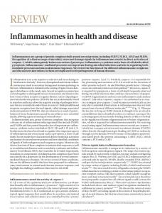
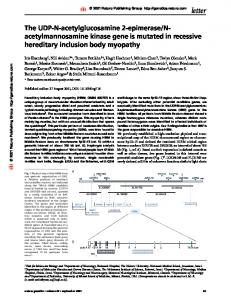
The starting point: We prove that coN P ⊆ IP by presenting an interactive proof system for the set of unsatisfiable CNF formulae, which is coN P-complete. Thus, our starting point is a given Boolean CNF formula, which is claimed to be unsatisfiable. Arithmetization of Boolean (CNF) formulae: Given a Boolean (CNF) formula, we replace the Boolean variables by integer variables, and replace the logical operations by corresponding arithmetic operations. In particular, the Boolean values false and true are replaced by the integer values 0 and 1 (respectively), or-clauses are replaced by sums, and the top level conjunction is replaced by a product. This translation is depicted in Figure 1.1. Note that the Boolean formula

variable values connectives final values

Boolean false, true ¬x, ∨ and ∧ false, true

arithmetic 0, 1 1 − x, + and · 0, positive

Figure 1.1: Arithmetization of CNF formulae. is satisfied (resp., unsatisfied) by a specific truth assignment if and only if evaluating the resulting arithmetic expression at the corresponding 0-1 assignment yields a positive (integer) value (resp., yields the value zero). Thus, the claim that the original Boolean formula is unsatisfiable translates to the claim that the summation of the resulting arithmetic expression, over all 0-1 assignments to its variables, yields the value zero. We highlight two additional observations regarding the resulting arithmetic expression: 1. The arithmetic expression is a low degree polynomial over the integers; specifically, its (total) degree equals the number of clauses in the original Boolean formula. 2. For any Boolean formula, the value of the corresponding arithmetic expression (for any choice of x1 , ..., xn ∈ {0, 1}) resides within the interval [0, v m ], where v is the maximum number of variables in a clause, and m is the number of clauses. Thus, summing over all 2n possible 0-1 assignments, where n ≤ vm is the number of variables, yields an integer value in [0, 2n v m ]. Moving to a Finite Field: In general, whenever we need to check equality between two integers in [0, M ], it suffices to check their equality mod q, where q > M . The benefit is that, if q is prime then the arithmetic is now in a finite field (mod q), and so certain things are “nicer” (e.g., uniformly selecting a value). Thus, proving that a CNF formula is not satisfiable reduces to proving an equality

12

of the following form X

···

x1 =0,1

X

φ(x1 , ..., xn ) ≡ 0

(mod q),

(1.1)

xn =0,1

where φ is a low-degree multi-variate polynomial (and q can be represented using O(|φ|) bits). In the rest of this exposition, all arithmetic operations refer to the finite field of q elements, denoted GF(q). Overview of the actual protocol: stripping summations in iterations. Given a formal expression as in Eq. (1.1), we strip off summations in iterations, stripping a single summation at each iteration, and instantiate the corresponding free variable as follows. At the beginning of each iteration the prover is supposed to supply the univariate polynomial representing the residual expression as a function of the (single) currently stripped variable. (By Observation 1, this is a low degree polynomial and so it has a short description.)5 The verifier checks that the polynomial (say, p) is of low degree, and that it corresponds to the current value (say, v) being claimed (i.e., it verifies that p(0) + p(1) ≡ v). Next, the verifier randomly instantiates the currently free variable (i.e., it selects uniformly r ∈ GF(q)), yielding a new value to be claimed for the resulting expression (i.e., the verifier computes v ← p(r), and expects a proof that the residual expression equals v). The verifier sends the uniformly chosen instantiation (i.e., r) to the prover, and the parties proceed to the next iteration (which refers to the residual expression and to the new value v). At the end of the last iteration, the verifier has a closed form expression (i.e., an expression without formal summations), which can be easily checked against the claimed value. A single iteration (detailed): The ith iteration is aimed at proving a claim of the form X X ··· φ(r1 , ..., ri−1 , xi , xi+1 , ..., xn ) ≡ vi−1 (mod q), (1.2) xi =0,1

xn =0,1

where v0 = 0, and r1 , ..., ri−1 and vi−1 are as determined in previous iterations. The ith iteration consists of two steps (messages): a prover step followed by a verifier step. The prover is supposed to provide the verifier with the univariate polynomial pi that satisfies X X def pi (z) = ··· φ(r1 , ..., ri−1 , z, xi+1 , ..., xn ) mod q . (1.3) xi+1 =0,1

xn =0,1

Note that, modulo q, the value pi (0) + pi (1) equals the l.h.s of Eq. (1.2). Denote by p0i the actual polynomial sent by the prover (i.e., the honest prover sets p0i = pi ). Then, the verifier first checks if p0i (0) + p0i (1) ≡ vi−1 (mod q), and next uniformly 5 We also use Observation 2, which implies that we may use a finite field with elements having a description length that is polynomial in the length of the original Boolean formula (i.e., log2 q = O(vm)).

13

selects ri ∈ GF(q) and sends it to the prover. Needless to say, the verifier will reject if the first check is violated. The claim to be proved in the next iteration is X X ··· φ(r1 , ..., ri−1 , ri , xi+1 , ..., xn ) ≡ vi (mod q), (1.4) xi+1 =0,1

xn =0,1

def

where vi = p0i (ri ) mod q is computed by each party. Completeness of the protocol: When the initial claim (i.e., Eq. (1.1)) holds, the prover can supply the correct polynomials (as determined in Eq. (1.3)), and this will lead the verifier to always accept. Soundness of the protocol: It suffices to upper-bound the probability that, for a particular iteration, the entry claim (i.e., Eq. (1.2)) is false while the ending claim (i.e., Eq. (1.4)) is valid. Indeed, let us focus on the ith iteration, and let vi−1 and pi be as in Eq. (1.2) and Eq. (1.3), respectively; that is, vi−1 is the (wrong) value claimed at the beginning of the ith iteration and pi is the polynomial representing the expression obtained when stripping the current variable (as in Eq. (1.3)). Let p0i (·) be any potential answer by the prover. We may assume, without loss of generality, that pi0 (0) + p0i (1) ≡ vi−1 (mod q) and that p0i is of low degree (since otherwise the verifier will definitely reject). Using our hypothesis (that the entry claim of Eq. (1.2) is false), we know that pi (0) + pi (1) 6≡ vi−1 (mod q). Thus, p0i and pi are different low-degree polynomials, and so they may agree on very few points (if at all). Now, if the verifier’s instantiation (i.e., its choice of a random ri ) does not happen to be one of these few points (i.e., pi (ri ) 6≡ p0i (ri ) (mod q)), then the ending claim (i.e., Eq. (1.4)) is false too (because the new value (i.e., vi ) is set to p0i (ri ) mod q, while the residual expression evaluates to pi (ri )). This establishes that the set of unsatisfiable CNF formulae has an interactive proof system. Actually, a similar proof system can be used to prove that a given formula has a given number of satisfying assignments; i.e., prove membership in the (“counting”) set {(φ, k) : |{τ : φ(τ ) = 1}| = k} . (1.5) Using adequate reductions, it follows that every problem in #P has an interactive proof system (i.e., for every NP-relation R, the set {(x, k) : |{y : (x, y) ∈ R}| = k} is in IP). Proving that PSPACE ⊆ IP requires a little more work, as outlined next. Obtaining interactive proofs for PSPACE (the basic idea). We present an interactive proof for the set of satisfied Quantified Boolean Formulae (QBF), which is complete for PSPACE. Recall that the number of quantifiers in such formulae is unbounded (e.g., it may be polynomially related to the length of the input), that there are both existential and universal quantifiers, and furthermore these quantifiers may alternate. In the arithmetization of these formulae, we replace existential quantifiers by summations and universal quantifiers by products. Two

14

difficulties arise when considering the application of the foregoing protocol to the resulting arithmetic expression. Firstly, the (integral) value of the expression (which may involve a big number of nested formal products) is only upper-bounded by a double-exponential function (in the length of the input). Secondly, when stripping a summation (or a product), the expression may be a polynomial of high degree (due to nested formal products that may appear in the remaining expression). For example, both phenomena occur in the following expression X Y Y ··· (x + yn ) , x=0,1 y1 =0,1

yn =0,1

P n−1 2n−1 which equals · (1 + x)2 . The first difficulty is easy to resolve x=0,1 x by using the fact that if two integers in [0, M ] are different then they must be different modulo most of the primes in the interval [3, poly(log M )]. Thus, we let the verifier select a random prime q of length that is linear in the length of the original formula, and the two parties consider the arithmetic expression reduced modulo this q. The second difficulty is resolved by noting that PSPACE is actually reducible to a special form of (non-canonical) QBF in which no variable appears both to the left and to the right of more than one universal quantifier. It follows that when arithmetizing and stripping summations (or products) from the resulting arithmetic expression, the corresponding univariate polynomial is of low degree (i.e., at most twice the length of the original formula, where the factor of two is due to the single universal quantifier that has this variable quantified on its left and appearing on its right). IP is contained in PSPACE: We shall show that, for every interactive proof system, there exists an optimal prover strategy that can be implemented in polynomialspace, where an optimal prover strategy is one that maximizes the probability that the prescribed verifier accepts the common input. It follows that IP ⊆ PSPACE, because (for every S ∈ IP) we can emulate, in polynomial space, all possible interactions of the prescribed verifier with any fixed polynomial-space prover strategy (e.g., an optimal one), and accept if and only if the majority of these interactions accept. Proposition 1.5 Let V be a probabilistic polynomial-time (verifier) strategy. Then, there exists a polynomial-space computable (prover) strategy f that, for every x, maximizes the probability that V accepts x. That is, for every P ∗ and every x it holds that the probability that V accepts x after interacting with P ∗ is upper-bounded by the probability that V accepts x after interacting with f . Proof Idea: The strategy f can be defined recursively. Specifically, for each partial transcript of the interaction with V , the next message of f is determined such that the probability that V accepts the common input (when the subsequent prover messages are determined by f ) is maximized.

15

1.4

Variants and finer structure: an overview

In this section we consider several variants on the basic definition of interactive proofs as well as finer complexity measures.

1.4.1

Arthur-Merlin games a.k.a public-coin proof systems

The verifier’s messages in a general interactive proof system are determined arbitrarily (but efficiently) based on the verifier’s view of the interaction so far (which includes its internal coin tosses, which without loss of generality can take place at the onset of the interaction). Thus, the verifier’s past coin tosses are not necessarily revealed by the messages that it sends. In contrast, in public-coin proof systems (a.k.a Arthur-Merlin proof systems), the verifier’s messages contain the outcome of any coin that it tosses at the current round. Thus, these messages reveal the randomness used towards generating them (i.e., this randomness becomes public). Actually, without loss of generality, the verifier’s messages can be identical to the outcome of the coins tossed at the current round (because any other string that the verifier may compute based on these coin tosses is actually determined by them). Note that the proof systems presented in the proof of Theorem 1.4 are of the public-coin type, whereas this is not the case for the Graph Non-Isomorphism proof system (of Construction 1.3). Thus, although not all natural proof systems are of the public-coin type, by Theorem 1.4 every set having an interactive proof system also has a public-coin interactive proof system. This means that, in the context of interactive proof systems, asking random questions is as powerful as asking clever questions. (A stronger statement appears at the end of Sec. 1.4.3.) Indeed, public-coin proof systems are a syntactically restricted type of interactive proof systems. This restriction may make the design of such systems more difficult, but potentially facilitates their analysis (and especially when the analysis refers to a generic system). Another advantage of public-coin proof systems is that the verifier’s actions (except for its final decision) are oblivious of the prover’s messages. This property is used in the proof of Theorem 2.6.

1.4.2

Interactive proof systems with two-sided error

In Definition 1.1 error probability is allowed in the soundness condition but not in the completeness condition. In such a case, we say that the proof system has perfect completeness (or one-sided error probability). A more general definition allows an error probability (upper-bounded by, say, 1/3) in both the completeness and the soundness conditions. Note that sets having such generalized (two-sided error) interactive proofs are also in PSPACE, and thus (by Theorem 1.4) allowing twosided error does not increase the power of interactive proofs. See further discussion at the end of Sec. 1.4.3.

16

1.4.3

A hierarchy of interactive proof systems

Definition 1.1 only refers to the total computation time of the verifier, and thus allows an arbitrary (polynomial) number of messages to be exchanged. A finer definition refers to the number of messages being exchanged (also called the number of rounds).6 Definition 1.6 (The round-complexity of interactive proofs): • For an integer function m, the complexity class IP(m) consists of sets having an interactive proof system in which, on common input x, at most m(|x|) messages are exchanged between the parties.7 def S • For a set of integer functions, M , we let IP(M ) = m∈M IP(m). Thus, IP = IP(poly). For example, interactive proof systems in which the verifier sends a single message that is answered by a single message of the prover corresponds to IP(2). Clearly, N P ⊆ IP(1), yet the inclusion may be strict because in IP(1) the verifier may toss coins after receiving the prover’s single message. (Also note that IP(0) = coRP.) Definition 1.6 gives rise to a natural hierarchy of interactive proof systems, where different “levels” of this hierarchy correspond to different “growth rates” of the round-complexity of these systems. The following results are known regarding this hierarchy. • A linear speed-up (see [6] and [33]): For every integer function, f , such that f (n) ≥ 2 for all n, the class IP(O(f (·))) collapses to the class IP(f (·)). In particular, IP(O(1)) collapses to IP(2). • The class IP(2) contains sets that are not known to be in N P; e.g., Graph Non-Isomorphism (see Construction 1.3). However, under plausible intractability assumptions, IP(2) = N P (see [42]). • If coN P ⊆ IP(2) then the Polynomial-Time Hierarchy collapses (see [15]). It is conjectured that coN P is not contained in IP(2), and consequently that interactive proofs with an unbounded number of message exchanges are more powerful than interactive proofs in which only a bounded (i.e., constant) number of messages are exchanged.8 The class IP(1), also denoted MA, seems to be the “real” randomized (and yet non-interactive) version of N P: Here the prover supplies a candidate (polynomialsize) “proof”, and the verifier assesses its validity probabilistically (rather than deterministically). 6 An even finer structure emerges when considering also the total length of the messages sent by the prover (see [31]). 7 We count the total number of messages exchanged, regardless of the direction of communication. Note that, without loss of generality, the last message is sent by the prover, the penultimate message is sent by the verifier, etc. 8 Note that the linear speed-up cannot be applied for an unbounded number of times, because each application may increase (e.g., square) the time-complexity of verification.

17

The IP-hierarchy (i.e., IP(·)) equals an analogous hierarchy, denoted AM(·), that refers to public-coin (a.k.a Arthur-Merlin) interactive proofs. That is, for every integer function f , it holds that AM(f ) = IP(f ). For f ≥ 1, it is also the case that AM(2f ) = AM(O(f )); actually, the aforementioned linear speed-up for IP(·) is established by combining the following two results: 1. Emulating IP(·) by AM(·): IP(f ) ⊆ AM(f + 3) [33]. 2. Linear speed-up for AM(·): AM(2f + 1) ⊆ AM(f + 1) [6]. In particular, IP(O(1)) = AM(2), even if AM(2) is restricted such that the verifier tosses no coins after receiving the prover’s message. (Note that IP(1) = AM(1) and IP(0) = AM(0) are trivial.) We comment that it is common to shorthand AM(2) by AM, which is indeed inconsistent with the convention of using IP as shorthand of IP(poly). The fact that IP(O(f )) = IP(f ) is proved by establishing an analogous result for AM(·) demonstrates the advantage of the public-coin setting for the study of interactive proofs. A similar phenomenon occurs when establishing that the IP-hierarchy equals an analogous two-sided error hierarchy [23].

1.4.4

Something completely different

We stress that although we have relaxed the requirements from the verification procedure (by allowing it to interact with the prover, toss coins, and risk some (bounded) error probability), we did not restrict the soundness of its verdict by assumptions concerning the potential prover(s). This should be contrasted with other notions of proof systems, such as computationally-sound ones (see Sec. 1.5.2), in which the soundness of the verifier’s verdict depends on assumptions concerning the potential prover(s).

1.5

On computationally bounded provers: an overview

Recall that our definition of interactive proofs (i.e., Definition 1.1) makes no reference to the computational abilities of the potential prover. This fact has two opposite consequences: 1. The completeness condition does not provide any upper bound on the complexity of the corresponding proving strategy (which convinces the verifier to accept valid assertions). 2. The soundness condition guarantees that, regardless of the computational effort spend by a cheating prover, the verifier cannot be fooled to accept invalid assertions (with probability exceeding the soundness error). Note that providing an upper-bound on the complexity of the (prescribed) prover strategy P of a specific interactive proof system (P, V ) only strengthens the claim that (P, V ) is an interactive proof system for the corresponding set (of valid assertions). We stress that the prescribed prover strategy is referred to only in the 18

completeness condition (and is irrelevant to the soundness condition). On the other hand, relaxing the definition of interactive proofs such that soundness holds only for a specific class of cheating prover strategies (rather than for all cheating prover strategies) weakens the corresponding claim. In this advanced section we consider both possibilities.

1.5.1

How powerful should the prover be?

Suppose that a set S is in IP. This means that there exists a verifier V that can be convinced to accept any input in S but cannot be fooled to accept any input not in S (except with small probability). One may ask how powerful should a prover be such that it can convince the verifier V to accept any input in S. Note that Proposition 1.5 asserts that an optimal prover strategy (for convincing any fixed verifier V ) can be implemented in polynomial-space, and we cannot expect any better for a generic set in PSPACE = IP. Still, we may seek better upper-bounds on the complexity of some prover strategy that convinces a specific verifier, which in turn corresponds to a specific set S. More interestingly, considering all possible verifiers that give rise to interactive proof systems for S, we wish to upper-bound the computational power that suffices for convincing any of these verifiers (to accept any input in S). We stress that, unlike the case of computationally-sound proof systems (see Sec. 1.5.2), we do not restrict the power of the prover in the soundness condition, but rather consider the minimum complexity of provers meeting the completeness condition. Specifically, we are interested in relatively efficient provers that meet the completeness condition. The term “relatively efficient prover” has been given three different interpretations, which are briefly surveyed next. 1. A prover is considered relatively efficient if, when given an auxiliary input (in addition to the common input in S), it works in (probabilistic) polynomialtime. Specifically, in case S ∈ N P, the auxiliary input maybe an NP-proof that the common input is in the set. Still, even in this case the interactive proof need not consist of the prover sending the auxiliary input to the verifier; for example, an alternative procedure may allow the prover to be zero-knowledge (see Construction 2.4). This interpretation is adequate and in fact crucial for applications in which such an auxiliary input is available to the otherwise polynomial-time parties. Typically, such auxiliary input is available in cryptographic applications in which parties wish to prove in (zero-knowledge) that they have correctly conducted some computation. In these cases, the NP-proof is just the transcript of the computation by which the claimed result has been generated, and thus the auxiliary input is available to the party that plays the role of the prover. 2. A prover is considered relatively efficient if it can be implemented by a probabilistic polynomial-time oracle machine with oracle access to the set S itself. Note that the prover in Construction 1.3 has this property.

19

This interpretation generalizes the notion of self-reducibility of NP-proof systems. Recall that by self-reducibility of an NP-set (or rather of the corresponding NP-proof system) we mean that the search problem of finding an NP-witness is polynomial-time reducible to deciding membership in the set. Here we require that implementing the prover strategy (in the relevant interactive proof) be polynomial-time reducible to deciding membership in the set. 3. A prover is considered relatively efficient if it can be implemented by a probabilistic machine that runs in time that is polynomial in the deterministic complexity of the set. This interpretation relates the time-complexity of convincing a “lazy person” (i.e., a verifier) to the time-complexity of determining the truth (i.e., deciding membership in the set). Hence, in contrast to the first interpretation, which is adequate in settings where assertions are generated along with their NP-proofs, the current interpretation is adequate in settings in which the prover is given only the assertion and has to test its validity by itself (before trying to convince a lazy verifier of this claim).

1.5.2

Computational Soundness

Relaxing the soundness condition such that it only refers to relatively efficient ways of trying to fool the verifier (rather than to all possible ways) yields a fundamentally different notion of a proof system. The verifier’s verdict in such a system is not absolutely sound, but is rather sound provided that the potential cheating prover does not exceed the presumed complexity limits. As in Sec. 1.5.1, the notion of “relative efficiency” can be given different interpretations, the most popular one being that the cheating prover strategy can be implemented by a (non-uniform) family of polynomial-size circuits. The latter interpretation coincides with the first interpretation used in Sec. 1.5.1 (i.e., a probabilistic polynomial-time strategy that is given an auxiliary input (of polynomial length)). Specifically, in this case, the soundness condition is replaced by the following computational soundness condition that asserts that it is infeasible to fool the verifier into accepting false statements. Formally: For every prover strategy that is implementable by a family of polynomialsize circuits {Cn }, and every sufficiently long x ∈ {0, 1}∗ \ S, the probability that V accepts x when interacting with C|x| is less than 1/2. As in case of standard soundness, the computational-soundness error can be reduced by repetitions. We warn, however, that unlike in the case of standard soundness (where both sequential and parallel repetitions will do), the computationalsoundness error cannot always be reduced by parallel repetitions (see [9, 45]). It is common and natural to consider proof systems in which the prover strategies considered both in the completeness and soundness conditions satisfy the same notion of relative efficiency. Protocols that satisfy these conditions with respect 20

to the foregoing interpretation are called arguments. We mention that argument systems may be more efficient (e.g., in terms of their communication complexity) than interactive proof systems (see [39] versus [31]).

21

Chapter 2

Zero-Knowledge Proof Systems Standard mathematical proofs are believed to yield (extra) knowledge and not merely establish the validity of the assertion being proved; that is, it is commonly believed that (good) proofs provide a deeper understanding of the theorem being proved. At the technical level, an NP-proof of membership in some set S ∈ N P \ P yields something (i.e., the NP-proof itself) that is hard to compute (even when assuming that the input is in S). For example, a 3-coloring of a graph constitutes an NP-proof that the graph is 3-colorable, but it yields information (i.e., the coloring) that seems infeasible to compute (when given an arbitrary 3-colorable graph). A natural question that arises is whether or not proving an assertion always requires giving away some extra knowledge. The setting of interactive proof systems enables a negative answer to this fundamental question: In contrast to NP-proofs, which seem to yield a lot of knowledge, zero-knowledge (interactive) proofs yield no knowledge at all; that is, zero-knowledge proofs are both convincing and yet yield nothing beyond the validity of the assertion being proved. For example, a zeroknowledge proof of 3-colorability does not yield any information about the graph (e.g., partial information about a 3-coloring) that is infeasible to compute from the graph itself. Thus, zero-knowledge proofs exhibit an extreme contrast between being convincing (of the validity of an assertion) and teaching anything on top of the validity of the assertion. Needless to say, the notion of zero-knowledge proofs is fascinating (e.g., since it differentiates proof-verification from learning). Still, the reader may wonder whether such a phenomenon is desirable, because in many settings we do care to learn as much as possible (rather than learn as little as possible). However, in other settings (most notably in cryptography), we may actually wish to limit the gain that other parties may obtain from a proof (and, in particular, limit this gain to the minimal level of being convinced of the validity of the assertion). Indeed, the applicability of zero-knowledge proofs in the domain of cryptography is vast; they are typically used as a tool for forcing (potentially malicious) parties

22

to behave according to a predetermined protocol (without having them reveal their own private inputs). The interested reader is referred to detailed treatments in [25, 26]. We also mention that, in addition to their direct applicability in cryptography, zero-knowledge proofs serve as a good benchmark for the study of various questions regarding cryptographic protocols.

2.1

Definitional Issues

Loosely speaking, zero-knowledge proofs are proofs that yield nothing beyond the validity of the assertion; that is, a verifier obtaining such a proof only gains conviction in the validity of the assertion. This is formulated by saying that anything that can be feasibly obtained from a zero-knowledge proof is also feasibly computable from the (valid) assertion itself. The latter formulation follows the simulation paradigm, which is discussed next.

2.1.1

A wider perspective: the simulation paradigm

In defining zero-knowledge proofs, we view the verifier as a potential adversary that tries to gain knowledge from the (prescribed) prover.1 We wish to state that no (feasible) adversary strategy for the verifier can gain anything from the prover (beyond conviction in the validity of the assertion). The question addressed here is how to formulate the “no gain” requirement. Let us consider the desired formulation from a wide perspective. A key question regarding the modeling of security concerns is how to express the intuitive requirement that an adversary “gains nothing substantial” by deviating from the prescribed behavior of an honest user. The answer is that the adversary gains nothing if whatever it can obtain by unrestricted adversarial behavior can be obtained within essentially the same computational effort by a benign (or prescribed) behavior. The definition of the “benign behavior” captures what we want to achieve in terms of security, and is specific to the security concern to be addressed. For example, in the context of zero-knowledge, a benign behavior is any computation that is based (only) on the assertion itself (while assuming that the latter is valid). Thus, a zero-knowledge proof is an interactive proof in which no feasible adversarial verifier strategy can obtain from the interaction more than a “benign party” (which believes the assertion) can obtain from the assertion itself. The foregoing interpretation of “gaining nothing” means that any feasible adversarial behavior can be “simulated” by a benign behavior (and thus there is no gain in the former). This line of reasoning is called the simulation paradigm, and is pivotal to many definitions in cryptography (e.g., it underlies the definitions of security of encryption schemes and cryptographic protocols; see [26]). 1 Recall that when defining a proof system (e.g., an interactive proof system), we view the prover as a potential adversary that tries to fool the (prescribed) verifier (into accepting invalid assertions).

23

2.1.2

The basic definitions

We turn back to the concrete task of defining zero-knowledge. Firstly, we comment that zero-knowledge is a property of some prover strategies; actually, more generally, zero-knowledge is a property of some strategies. Fixing any strategy (e.g., a prescribed prover), we consider what can be gained (i.e., computed) by an arbitrary feasible adversary (e.g., a verifier) that interacts with the aforementioned fixed strategy on a common input taken from a predetermined set (in our case, the set of valid assertions). This gain is compared against what can be computed by an arbitrary feasible algorithm (called a simulator) that is only given the input itself. The fixed strategy is zero-knowledge if the “computational power” of these two (fundamentally different settings) is essentially equivalent. Details follow. The formulation of the zero-knowledge condition refers to two types of probability ensembles, where each ensemble associates a single probability distribution to each relevant input (e.g., a valid assertion). Specifically, in the case of interactive proofs, the first ensemble represents the output distribution of the verifier after interacting with the specified prover strategy P (on some common input), where the verifier is employing an arbitrary efficient strategy (not necessarily the specified one). The second ensemble represents the output distribution of some probabilistic polynomial-time algorithm (which is only given the corresponding input (and does not interact with anyone)). The basic paradigm of zero-knowledge asserts that for every ensemble of the first type there exist a “similar” ensemble of the second type. The specific variants differ by the interpretation given to the notion of similarity. The most strict interpretation, leading to perfect zero-knowledge, is that similarity means equality. Definition 2.1 (perfect zero-knowledge, over-simplified):2 A prover strategy, P , is said to be perfect zero-knowledge over a set S if for every probabilistic polynomialtime verifier strategy, V ∗ , there exists a probabilistic polynomial-time algorithm, A∗ , such that (P, V ∗ )(x) ≡ A∗ (x) , for every x ∈ S where (P, V ∗ )(x) is a random variable representing the output of verifier V ∗ after interacting with the prover P on common input x, and A∗ (x) is a random variable representing the output of algorithm A∗ on input x. We comment that any set in coRP has a perfect zero-knowledge proof system in which the prover keeps silence and the verifier decides by itself. The same holds for BPP provided that we relax the definition of interactive proof system to allow two-sided error. Needless to say, our focus is on non-trivial proof systems; that is, proof systems for sets outside of BPP. 2 In the actual definition one relaxes the requirement in one of the following two ways. The first alternative is allowing A∗ to run for expected (rather than strict) polynomial-time. The second alternative consists of allowing A∗ to have no output with probability at most 1/2 and considering the value of its output conditioned on it having output at all. The latter alternative implies the former, but the converse is not known to hold.

24

A somewhat more relaxed interpretation (of the notion of similarity), leading to almost-perfect zero-knowledge (a.k.a statistical zero-knowledge), is that similarity means statistical closeness (i.e., negligible difference between the ensembles). The most liberal interpretation, leading to the standard usage of the term zeroknowledge (and sometimes referred to as computational zero-knowledge), is that similarity means computational indistinguishability (i.e., failure of any efficient procedure to tell the two ensembles apart). Combining the foregoing discussion with the relevant definition of computational indistinguishability (cf. [27, Sec. C.3.1]), we obtain the following definition. Definition 2.2 (zero-knowledge, somewhat simplified): A prover strategy, P , is said to be zero-knowledge over a set S if for every probabilistic polynomial-time verifier strategy, V ∗ , there exists a probabilistic polynomial-time simulator, A∗ , such that for every probabilistic polynomial-time distinguisher, D, it holds that def

d(n) =

max

x∈S∩{0,1}n

{|Pr[D(x, (P, V ∗ )(x)) = 1] − Pr[D(x, A∗ (x)) = 1]|}

is a negligible function.3 We denote by ZK the class of sets having zero-knowledge interactive proof systems. Definition 2.2 is a simplified version of the actual definition (presented, e.g., in [25, Sec. 4.3.3]). Specifically, in order to guarantee that zero-knowledge is preserved under sequential composition it is necessary to slightly augment the definition (by providing V ∗ and A∗ with the same value of an arbitrary (poly(|x|)-bit long) auxiliary input). On the role of randomness and interaction. It can be shown that only sets in BPP have zero-knowledge proofs in which the verifier is deterministic. The same holds for deterministic provers, provided that we consider “auxiliary-input” zero-knowledge. It can also be shown that only sets in BPP have zero-knowledge proofs in which a single message is sent. Thus, both randomness and interaction are essential to the non-triviality of zero-knowledge proof systems. (For further details, see [25, Sec. 4.5.1].) Advanced Comment: Knowledge Complexity. Zero-knowledge is the lowest level of a knowledge-complexity hierarchy which quantifies the “knowledge revealed in an interaction.” Specifically, the knowledge complexity of an interactive proof system may be defined as the minimum number of oracle-queries required in order to efficiently simulate an interaction with the prover (see [30]). 3 That

is, d vanishes faster that the reciprocal of any positive polynomial (i.e., for every positive def

polynomial p and for sufficiently large n, it holds that d(n) < 1/p(n)). Needless to say, d(n) = 0 if S ∩ {0, 1}n = ∅.

25

2.2

The Power of Zero-Knowledge

When faced with a definition as complex (and seemingly self-contradictory) as the definition of zero-knowledge, one should indeed wonder whether the definition can be met (in a non-trivial manner).4 It turns out that the existence of non-trivial zero-knowledge proofs is related to the existence of intractable problems in N P. In particular, we will show that if one-way functions exist then every NP-set has a zero-knowledge proof system. (For the converse, see [25, Sec. 4.5.2] or [50].) But first, we demonstrate the non-triviality of zero-knowledge by a presenting a simple (perfect) zero-knowledge proof system for a specific NP-set that is not known to be in BPP. In this case we make no intractability assumptions (yet, the result is significant only if N P is not contained in BPP).

2.2.1

A simple example

Recall that the set of pairs of isomorphic graphs is not known to be in BPP, and thus the straightforward NP-proof system (in which the prover just supplies the isomorphism) may not be zero-knowledge. Furthermore, assuming that Graph Isomorphism is not in BPP, this set has no zero-knowledge NP-proof system. Still, as we shall shortly see, this set does have a zero-knowledge interactive proof system.5 Construction 2.3 (zero-knowledge proof for Graph Isomorphism): • Common Input: A pair of graphs, G1 = (V1 , E1 ) and G2 = (V2 , E2 ). If the input graphs are indeed isomorphic, then we let φ denote an arbitrary isomorphism between them; that is, φ is a 1-1 and onto mapping of the vertex set V1 to the vertex set V2 such that {u, v} ∈ E1 if and only if {φ(v), φ(u)} ∈ E2 . • Prover’s first Step (P1): The prover selects a random isomorphic copy of G2 , and sends it to the verifier. Namely, the prover selects at random, with uniform probability distribution, a permutation π from the set of permutations over the vertex set V2 , and constructs a graph with vertex set V2 and edge set def

E = {{π(u), π(v)} : {u, v} ∈ E2 } . The prover sends (V2 , E) to the verifier. 4 Recall that any set in BPP has a trivial zero-knowledge (two-sided error) proof system in which the verifier just determines membership by itself. Thus, the issue is the existence of zeroknowledge proofs for sets outside BPP. 5 We mention that Construction 1.3 is zero-knowledge in a restricted sense (i.e., w.r.t the honest verifier), but is not known to be zero-knowledge (in the general sense). In particular, a cheating verifier may abuse the prover in order to learn whether or not G1 is isomorphic to some third graph (which may be either given to it as auxiliary input or generated by it based on the common input).

26

• Motivating Remark: If the input graphs are isomorphic, as the prover claims, then the graph sent in Step P1 is isomorphic to both input graphs. However, if the input graphs are not isomorphic then no graph can be isomorphic to both of them. • Verifier’s first Step (V1): Upon receiving a graph, G0 = (V 0 , E 0 ), from the prover, the verifier asks the prover to show an isomorphism between G0 and one of the input graphs, chosen at random by the verifier. Namely, the verifier uniformly selects σ ∈ {1, 2}, and sends it to the prover (who is supposed to answer with an isomorphism between Gσ and G0 ). • Prover’s second Step (P2): If the message, σ, received from the verifier equals 2 then the prover sends π to the verifier. Otherwise (i.e., σ 6= 2), the prover def

sends π ◦ φ (i.e., the composition of π on φ, defined as π ◦ φ(v) = π(φ(v))) to the verifier. (Indeed, the prover treats any σ 6= 2 as σ = 1. Thus, in the analysis we shall assume, without loss of generality, that σ ∈ {1, 2} always holds.) • Verifier’s second Step (V2): If the message, denoted ψ, received from the prover is an isomorphism between Gσ and G0 then the verifier outputs 1, otherwise it outputs 0. The verifier strategy in Construction 2.3 is easily implemented in probabilistic polynomial-time. If the prover is given an isomorphism between the input graphs as auxiliary input, then also the prover’s program can be implemented in probabilistic polynomial-time. The motivating remark justifies the claim that Construction 2.3 constitutes an interactive proof system for the set of pairs of isomorphic graphs. Thus, we focus on establishing the zero-knowledge property. We consider first the special case in which the verifier actually follows the prescribed strategy (and selects σ at random, and in particular obliviously of the graph G0 it receives). The view of this verifier can be easily simulated by selecting σ and ψ at random, constructing G0 as a random isomorphic copy of Gσ (via the isomorphism ψ), and outputting the triple (G0 , σ, ψ). Indeed (even in this case), the simulator behaves differently from the prescribed prover (which selects G0 as a random isomorphic copy of G2 , via the isomorphism π), but its output distribution is identical to the verifier’s view in the real interaction. However, the foregoing description assumes that the verifier follows the prescribed strategy, while in general the verifier may (adversarially) select σ depending on the graph G0 . Thus, a slightly more complicated simulation (described next) is required. A general clarification may be in place. Recall that we wish to simulate the interaction of an arbitrary verifier strategy with the prescribed prover. Thus, this simulator must depend on the corresponding verifier strategy, and indeed we shall describe the simulator while referring to such a generic verifier strategy. Formally, this means that the simulator’s program incorporates the program of the corresponding verifier strategy. Actually, the following simulator uses the generic verifier strategy as a subroutine.

27

Turning back to the specific protocol of Construction 2.3, the basic idea is that simulator tries to guess σ and completes a simulation if its guess turns out to be correct. Specifically, the simulator selects τ ∈ {1, 2} uniformly (hoping that the verifier will later select σ = τ ), and constructs G0 by randomly permuting Gτ (and thus being able to present an isomorphism between Gτ and G0 ). Recall that the simulator is analyzed only on yes-instances (i.e., the input graphs G1 and G2 are isomorphic). The point is that if G1 and G2 are isomorphic, then the graph G0 does not yield any information regarding the simulator’s guess (i.e., τ ).6 Thus, the value σ selected by the adversarial verifier may depend on G0 but not on τ , which implies that Pr[σ = τ ] = 1/2. In other words, the simulator’s guess (i.e., τ ) is correct (i.e., equals σ) with probability 1/2. Now, if the guess is correct then the simulator can produce an output that has the correct distribution, and otherwise the entire process is repeated. Digest: a few useful conventions. We highlight three conventions that were either used (implicitly) in the foregoing analysis or can be used to simplify the description of (this and/or) other zero-knowledge simulators. 1. Without loss of generality, we may assume that the cheating verifier strategy is implemented by a deterministic polynomial-size circuit (or, equivalently, by a deterministic polynomial-time algorithm with an auxiliary input).7 This is justified by fixing any outcome of the verifier’s coins, and observing that our (“uniform”) simulation of the various (residual) deterministic strategies yields a simulation of the original probabilistic strategy. 2. Without loss of generality, it suffices to consider cheating verifiers that (only) output their view of the interaction (i.e., the common input, their internal coin tosses, and the messages that they have received). In other words, it suffices to simulate the view that cheating verifiers have of the real interaction. This is justified by noting that the final output of any verifier can be obtained from its view of the interaction, where the complexity of the transformation is upper-bounded by the complexity of the verifier’s strategy. 3. Without loss of generality, it suffices to construct a “weak simulator” that produces output with some noticeable8 probability such that whenever an output is produced it is distributed “correctly” (i.e., similarly to the distribution occuring in real interactions with the prescribed prover). This is justified by repeatedly invoking such a weak simulator (polynomially) many times and using the first output produced by any of these invocations. Note that by using an adequate number of invocations, we fail to produce 6 Indeed, this observation is identical to the observation made in the analysis of the soundness of Construction 1.3. 7 This observation is not crucial, but it does simplify the analysis (by eliminating the need to specify a sequence of coin tosses in each invocation of the verifier’s strategy). 8 A probability is called noticeable if it is greater than the reciprocal of some positive polynomial (in the relevant parameter).

28

an output with negligible probability. Furthermore, note that a simulator that fails to produce output with negligible probability can be converted to a simulator that always produces an output, while incurring a negligible statistic deviation in the output distribution.

2.2.2

The full power of zero-knowledge proofs

The zero-knowledge proof system presented in Construction 2.3 refers to one specific NP-set that is not known to be in BPP. It turns out that, under reasonable assumptions, zero-knowledge can be used to prove membership in any NP-set. Intuitively, it suffices to establish this fact for a single NP-complete set, and thus we focus on presenting a zero-knowledge proof system for the set of 3-colorable graphs. This proof system will be described while referring to “boxes” in which information can be hidden and later revealed. Such boxes can be implemented using one-way functions (see Theorem 2.5). Construction 2.4 (Zero-knowledge proof of 3-colorability, abstract description): The description refers to abstract non-transparent boxes that can be perfectly locked and unlocked such that these boxes perfectly hide their contents while being locked. • Common Input: A simple graph G = (V, E). • Prover’s first step: Let ψ be a 3-coloring of G. The prover selects a random def permutation, π, over {1, 2, 3}, and sets φ(v) = π(ψ(v)), for each v ∈ V . Hence, the prover forms a random relabeling of the 3-coloring ψ. The prover sends to the verifier a sequence of |V | locked and non-transparent boxes such that the v th box contains the value φ(v). • Verifier’s first step: The verifier uniformly selects an edge {u, v} ∈ E, and sends it to the prover. • Motivating Remark: The boxes are supposed to contain a 3-coloring of the graph, and the verifier asks to inspect the colors of vertices u and v. Indeed, for the zero-knowledge condition, it is crucial that the prover only responds to pairs that correspond to edges of the graph. • Prover’s second step: Upon receiving an edge {u, v} ∈ E, the prover sends to the verifier the keys to boxes u and v. For simplicity of the analysis, if the verifier sends {u, v} 6∈ E then the prover behaves as if it has received a fixed (or random) edge in E, rather than suspending the interaction, which would have been the natural thing to do. • Verifier’s second step: The verifier unlocks and opens boxes u and v, and accepts if and only if they contain two different elements in {1, 2, 3}.

29

The verifier strategy in Construction 2.4 is easily implemented in probabilistic polynomial-time. The same holds with respect to the prover’s strategy, provided that it is given a 3-coloring of G as auxiliary input. Clearly, if the input graph is 3-colorable then the verifier accepts with probability 1 when interacting with the prescribed prover. On the other hand, if the input graph is not 3-colorable, then any contents put in the boxes must be invalid with respect to at least one edge, 1 and consequently the verifier will reject with probability at least |E| . Hence, the foregoing protocol exhibits a noticeable gap in the accepting probabilities between the case of 3-colorable graphs and the case of non-3-colorable graphs. To increase the gap, the protocol may be repeated sufficiently many times (of course, using independent coin tosses in each repetition). So far we showed that Construction 2.4 constitutes (a weak form of) an interactive proof system for Graph 3-Colorability. The point, however, is that the prescribed prover strategy is zero-knowledge. This is easy to see in the abstract setting of Construction 2.4, because all that the verifier sees in the real interaction is a sequence of boxes and a random pair of different colors (which is easy to simulate). Indeed, the simulation of the real interaction proceeds by presenting a sequence of boxes and providing a random pair of different colors as the contents of the two boxes indicated by the verifier. Note that the foregoing argument relies on the fact that the boxes (indicated by the verifier) correspond to vertices that are connected by an edge in the graph. This simple demonstration of the zero-knowledge property is not possible in the digital implementation (discussed next), because in that case the boxes are not totally unaffected by their contents (but are rather affected, yet in an indistinguishable manner). Thus, the verifier’s selection of the inspected edge may depend on the “outside appearance” of the various boxes, which in turn may depend (in an indistinguishable manner) on the contents of these boxes. Consequently, we cannot determine the boxes’ contents after a pair of boxes are selected, and so the simple foregoing simulation is inapplicable. Instead, we simulate the interaction as follows. 1. We first guess (at random) which pair of boxes (corresponding to an edge) the verifier would ask to open, and place a random pair of distinct colors in these boxes (and garbage in the rest).9 Then, we hand all boxes to the verifier, who asks us to open a pair of boxes (corresponding to an edge). 2. If the verifier asks for the pair that we chose (i.e., our guess is successful), then we can complete the simulation by opening these boxes. Otherwise, we try again (i.e., repeat Step 1 with a new random guess and random colors). The key observation is that if the boxes hide the contents in the sense that a box’s contents is indistinguishable based on its outside appearance, then our guess will succeed with probability approximately 1/|E|. Furthermore, 9 An alternative (and more efficient) simulation consists of putting random independent colors in the various boxes, hoping that the verifier asks for an edge that is properly colored. The latter event occurs with probability (approximately) 2/3, provided that the boxes hide their contents (almost) perfectly.

30

in this case, the simulated execution will be indistinguishable from the real interaction. Thus, it suffices to use boxes that hide their contents almost perfectly (rather than being perfectly opaque). Such boxes can be implemented digitally. Digital implementation (overview). We implement the abstract boxes (referred to in Construction 2.4) by using adequately defined commitment schemes. Loosely speaking, such a scheme is a two-phase game between a sender and a receiver such that after the first phase the sender is “committed” to a value and yet, at this stage, it is infeasible for the receiver to find out the committed value (i.e., the commitment is “hiding”). The committed value will be revealed to the receiver in the second phase and it is guaranteed that the sender cannot reveal a value other than the one committed (i.e., the commitment is “binding”). Such commitment schemes can be implemented assuming the existence of one-way functions (i.e., functions that are easy to evaluate but hard to invert even in the average-case sense). For details see, e.g., [25, Sec. 4.4.1]. Zero-knowledge proofs for other NP-sets. Using the fact that 3-colorability is NP-complete, one can derive (from Construction 2.4) zero-knowledge proof systems for any NP-set.10 Furthermore, these proof systems employ relatively efficient prover strategies. Theorem 2.5 (The ZK Theorem): Assuming the existence of (non-uniformly hard) one-way functions, it holds that N P ⊆ ZK. Furthermore, every S ∈ N P has a (computational) zero-knowledge interactive proof system in which the prescribed prover strategy can be implemented in probabilistic polynomial-time, provided that it is given as auxiliary-input an NP-witness for membership of the common input in S. The hypothesis of Theorem 2.5 (i.e., the existence of one-way functions) seems unavoidable, because the existence of zero-knowledge proofs for “hard on the average” problems implies the existence of one-way functions (see [50]). Theorem 2.5 has a dramatic effect on the design of cryptographic protocols (see, e.g., [26]). In a different vein we mention that, under the same assumption, any interactive proof can be transformed into a zero-knowledge one. (This transformation, however, does not necessarily preserve the complexity of the prover.) Theorem 2.6 (The ultimate ZK Theorem): Assuming the existence of (non-uniformly hard) one-way functions, it holds that IP = ZK. Loosely speaking, Theorem 2.6 can be proved by recalling that IP = AM(poly) and modifying any public-coin protocol as follows: the modified prover sends commitments to its messages rather than the messages themselves, and once the original interaction is completed it proves (in zero-knowledge) that the corresponding 10 Actually, we should either rely on the fact that the standard Karp-reductions are invertible in polynomial time or on the fact that the 3-colorability protocol is actually zero-knowledge with respect to auxiliary inputs.

31

transcript would have been accepted by the original verifier. Indeed, the latter assertion is of the “NP type”, and thus the zero-knowledge proof system guaranteed in Theorem 2.5 can be invoked for proving it. Reflection. The proof of Theorem 2.5 uses the fact that 3-colorability is NPcomplete in order to obtain a zero-knowledge proofs for any set in N P by using such a protocol for 3-colorability (i.e., Construction 2.4). Thus, an NP-completeness result is used here in a “positive” way; that is, in order to construct something rather than in order to derive a (“negative”) hardness result.11 Perfect and Statistical Zero-Knowledge. The foregoing results, which refer to computational zero-knowledge proof systems, should be contrasted with the known results regarding the complexity of statistical zero-knowledge proof systems: Statistical zero-knowledge proof systems exist only for sets in IP(2)∩coIP(2), and thus are unlikely to exist for all NP-sets. On the other hand, the class Statistical Zero-Knowledge is known to contain some seemingly hard problems, and turns out to have interesting complexity theoretic properties (e.g., being closed under complementation, and having very natural complete problems). The interested reader is referred to [49].

2.3

Proofs of Knowledge – a parenthetical section12

Loosely speaking, “proofs of knowledge” are interactive proofs in which the prover asserts “knowledge” of some object (e.g., a 3-coloring of a graph), and not merely its existence (e.g., the existence of a 3-coloring of the graph, which in turn is equivalent to the assertion that the graph is 3-colorable). Note that the entity asserting knowledge is actually the prover’s strategy, which is an automated computing device, hereafter referred to as a machine. This raises the question of what do we mean by saying that a machine knows something.

2.3.1

Abstract reflections

Any standard dictionary suggests several meanings for the verb to know, but these are typically phrased with reference to the notion of awareness, a notion which is certainly inapplicable in the context of machines. Instead, we should look for a behavioristic interpretation of the verb to know. Indeed, it is reasonable to link knowledge with the ability to do something (e.g., the ability to write down whatever one knows). Hence, we may say that a machine knows a string α if it can output the string α. But this seems as total non-sense too: a machine has a well defined 11 Historically, the proof of Theorem 2.5 was probably the first positive application of NPcompleteness. Subsequent positive uses of completeness results have appeared in the context of interactive proofs (see the proof of Theorem 1.4), probabilistically checkable proofs (see the proof of Theorem 3.3), and the study of statistical zero-knowledge (cf. [49]). 12 Technically speaking, this topic belongs to Chapter 1, but its more interesting demonstrations refer to zero-knowledge proofs of knowledge – hence its current positioning.

32

output – either the output equals α or it does not, so what can be meant by saying that a machine can do something? Interestingly, a sound interpretation of the latter phrase does exist. Loosely speaking, by saying that a machine can do something we mean that the machine can be easily modified such that it (or rather its modified version) does whatever is claimed. More precisely, this means that there exists an efficient machine that, using the original machine as a black-box (or given its code as an input), outputs whatever is claimed. Technically speaking, using a machine as a black-box seems more appealing when the said machine is interactive (i.e., implements an interactive strategy). Indeed, this will be our focus here. Furthermore, conceptually speaking, whatever a machine knows (or does not know) is its own business, whereas what can be of interest and reference to the outside is whatever can be deduced about the knowledge of a machine by interacting with it. Hence, we are interested in proofs of knowledge (rather than in mere knowledge).

2.3.2

A concrete treatment

For sake of simplicity let us consider a concrete question: how can a machine prove that it knows a 3-coloring of a graph? An obvious way is just sending the 3-coloring to the verifier. Yet, we claim that applying the protocol in Construction 2.4 (i.e., the zero-knowledge proof system for 3-Colorability) is an alternative way of proving knowledge of a 3-coloring of the graph. The definition of a verifier of knowledge of 3-coloring refers to any possible prover strategy and links the ability to “extract” a 3-coloring (of a given graph) from such a prover to the probability that this prover convinces the verifier. That is, the definition postulates the existence of an efficient universal way of “extracting” a 3-coloring of a given graph by using any prover strategy that convinces this verifier to accept this graph with probability 1 (or, more generally, with some noticeable probability). On the other hand, we should not expect this extractor to obtain much from prover strategies that fail to convince the verifier (or, more generally, convince it with negligible probability). A robust definition should allow a smooth transition between these two extremes (and in particular between provers that convince the verifier with noticeable probability and those that convince it with negligible probability). Such a definition should also support the intuition by which the following strategy of Alice is zero-knowledge: Alice sends Bob a 3-coloring of a given graph provided that Bob has successfully convinced her that he knows this coloring.13 We stress that the zero-knowledge property of Alice’s strategy should hold regardless of the proof-of-knowledge system used for proving Bob’s knowledge of a 3-coloring. Loosely speaking, we say that a strategy, V , constitutes a verifier for knowledge of 3-coloring if, for any prover strategy P , the complexity of extracting a 3-coloring 13 For simplicity, the reader may consider graphs that have a unique 3-coloring (up-to a relabeling). In general, we refer here to instances that have unique solution which arise naturally in some (cryptographic) applications.

33

of G when using P as a “black box”14 is inversely proportional to the probability that V is convinced by P (to accept the graph G). Namely, the extraction of the 3-coloring is done by an oracle machine, called an extractor, that is given access to the strategy P (i.e., the function specifying the message that P sends in response to any sequence of messages it may receive). We require that the (expected) running time of the extractor, on input G and oracle access to P , be inversely related (by a factor polynomial in |G|) to the probability that P convinces V to accept G. In particular, if P always convinces V to accept G, then the extractor runs in expected polynomial-time. The same holds in case P convinces V to accept with noticeable probability. On the other hand, if P never convinces V to accept, then nothing is required of the extractor. We stress that the latter special cases do not suffice for a satisfactory definition; see discussion in [25, Sec. 4.7.1]. Proofs of knowledge, and in particular zero-knowledge proofs of knowledge, have many applications to the design of cryptographic schemes and cryptographic protocols (see, e.g., [25, 26]). These are enabled by the following general result. Theorem 2.7 (Theorem 2.5, revisited): Assuming the existence of (non-uniformly hard) one-way functions, any NP-relation has a zero-knowledge proof of knowledge (of a corresponding NP-witnesses). Furthermore, the prescribed prover strategy can be implemented in probabilistic polynomial-time, provided it is given such an NP-witness.

14 Indeed,

one may consider also non-black-box extractors.

34

Chapter 3

Probabilistically Checkable Proof Systems Probabilistically checkable proof systems can be viewed as standard (deterministic) proof systems that are augmented with a probabilistic procedure capable of evaluating the validity of the assertion by examining few locations in the alleged proof. Actually, we focus on the latter probabilistic procedure, which in turn implies the existence of a deterministic verification procedure (obtained by going over all possible random choices of the probabilistic procedure and making the adequate examinations). Modeling such probabilistic verification procedures, which may examine few locations in the alleged proof, requires providing these procedures with direct access to the individual bits of the alleged proof (so that they need not scan the proof bit-by-bit). Thus, the alleged proof is a string, as in the case of a traditional proof system, but the (probabilistic) verification procedure is given direct access to individual bits of this string (see Figure 3.1). We are interested in probabilistic verification procedures that access only few locations in the proof, and yet are able to make a meaningful probabilistic verdict regarding the validity of the alleged proof. Specifically, the verification procedure should accept any valid proof (with probability 1), but rejects with probability at least 1/2 any alleged proof for a false assertion. Such probabilistic verification procedures are called probabilistically checkable proof (PCP) systems. The fact that one can (meaningfully) evaluate the correctness of proofs by examining few locations in them is indeed amazing and somewhat counter-intuitive. Needless to say, such proofs must be written in a somewhat non-standard format, because standard proofs cannot be verified without reading them in full (since a flaw may be due to a single improper inference). In contrast, proofs for a PCP system tend to be very redundant; they consist of superfluously many pieces of information (about the claimed assertion), but their correctness can be (meaningfully) evaluated by checking the consistency of a randomly chosen collection of few related pieces. We stress that by a “meaningful evaluation” we mean rejecting alleged proofs of

35

Figure 3.1: The PCP model – an illustration. false assertions with constant probability (rather than with probability that is inversely proportional to the length of the alleged proof). The main complexity measure associated with PCPs is indeed their query complexity. Another complexity measure of natural concern is the length of the proofs being employed, which in turn is related to the randomness complexity of the system. The randomness complexity of PCPs plays a key role in numerous applications (e.g., in composing PCP systems as well as when applying PCP systems to derive inapproximability results), and thus we specify this parameter rather than the proof length.

3.1

Definition

Loosely speaking, a probabilistically checkable proof system consists of a probabilistic polynomial-time verifier having access to an oracle that represents an alleged proof (in redundant form). Typically, the verifier accesses only few of the oracle bits, and these bit positions are determined by the outcome of the verifier’s coin tosses. As in the case of interactive proof systems, it is required that if the assertion holds then the verifier always accepts (i.e., when given access to an adequate oracle); whereas, if the assertion is false then the verifier must reject with probability at least 12 , no matter which oracle is used. The basic definition of the PCP setting is given in Part (1) of the following definition. Yet, the complexity measures introduced in Part (2) are of key importance for the subsequent discussions. Definition 3.1 (Probabilistically Checkable Proofs – PCP): 1. A probabilistically checkable proof system (PCP) for a set S is a probabilistic polynomial-time oracle machine, called verifier and denoted V , that satisfies the following two conditions: 36

• Completeness: For every x ∈ S there exists an oracle πx such that, on input x and access to oracle πx , machine V always accepts x. • Soundness: For every x 6∈ S and every oracle π, on input x and access to oracle π, machine V rejects x with probability at least 12 . 2. We say that a probabilistically checkable proof system has query complexity q : N → N if, on any input of length n, the verifier makes at most q(n) oracle queries.1 Similarly, the randomness complexity r : N → N upper-bounds the number of coin tosses performed by the verifier on a generic n-bit long input. For integer functions r and q, we denote by PCP(r, q) the class of sets having probabilistically checkable proof systems of randomness complexity r and query complexity q. For sets of integer functions, R and Q, [ def PCP(R, Q) = PCP(r, q) . r∈R , q∈Q

The error probability (in the soundness condition) of PCP systems can be reduced by successive applications of the proof system. In particular, repeating the process for k times, reduces the probability that the verifier is fooled by a false assertion to 2−k , whereas all complexities increase by at most a factor of k. Thus, PCP systems of non-trivial query-complexity (cf. Section 3.2) provide a trade-off between the number of locations examined in the proof and the confidence in the validity of the assertion. We note that the oracle πx referred to in the completeness condition of a PCP system constitutes a proof in the standard mathematical sense. Indeed any PCP system yields a standard proof system (with respect to a verification procedure that scans all possible outcomes of V ’s internal coin tosses and emulates all the corresponding checks). Furthermore, the oracles in PCP systems of logarithmic randomness-complexity constitute NP-proofs. However, the oracles of a PCP system have the extra remarkable property of enabling a lazy verifier to toss coins, take its chances and “assess” the validity of the proof without reading all of it (but rather by reading a tiny portion of it). Potentially, this allows the verifier to examine very few bits of an NP-proof and even utilize very long proofs (i.e., of super-polynomial length). Adaptive versus non-adaptive verifiers. Definition 3.1 allows the verifier to be adaptive; that is, the verifier may determine its queries based on the answers it has received to previous queries (in addition to their dependence on the input and on the verifier’s internal coin tosses). In contrast, non-adaptive verifiers determine all their queries based solely on their input andP internal coin tosses. q Note that q adaptive (binary) queries can be emulated by i=1 2i−1 < 2q nonadaptive (binary) queries. We comment that most constructions of PCP systems use non-adaptive verifiers, and in fact in many sources PCP systems are defined as non-adaptive. 1 As

usual in complexity theory, the oracle answers are binary values (i.e., either 0 or 1).

37

Randomness versus proof length. Fixing a verifier V , we say that location i (in the oracle) is relevant to input x if there exists a computation of V on input x in which location i is queried (i.e., there exists ω and π such that, on input x, randomness ω and access to the oracle π, the verifier queries location i). The effective proof length of V is the smallest function ` : N → N such that for every input x there are at most `(|x|) locations (in the oracle) that are relevant to x. We claim that the effective proof length of any PCP system is closely related to its randomness (and query) complexity. On one hand, if the PCP system has randomness-complexity r and query-complexity q, then its effective proof length is upper-bounded by 2r+q , whereas a bound of 2r · q holds for non-adaptive systems. Thus, PCP systems of logarithmic randomness complexity have effective proof length that is polynomial, and hence yield NP-proof systems. On the other hand, in some sense, the randomness complexity of a PCP system can be upper-bounded by the logarithm of the (effective) length of the proofs employed (provided we allow non-uniform verifiers). On the role of randomness. The PCP Theorem (i.e., N P ⊆ PCP(log, O(1))) asserts that a meaningful probabilistic evaluation of proofs is possible based on a constant number of examined bits. We note that, unless P = N P, such a phenomena is impossible when requiring the verifier to be deterministic. In particular, note that PCP(0, O(1)) = P holds (as a special case of PCP(r, q) ⊆ r Dtime(22 q+r · poly)).

3.2

The Power of Probabilistically Checkable Proofs

The celebrated PCP Theorem asserts that N P = PCP(log, O(1)), and this result is indeed the focus of the current section. But before getting to it we make several simple observations regarding the PCP Hierarchy. We first note that PCP(poly, 0) equals coRP, whereas PCP(0, poly) equals N P. It is easy to prove an upper bound on the non-deterministic time complexity of sets in the PCP hierarchy: Proposition 3.2 (upper-bounds on the power of PCPs): For every polynomially bounded integer function r, it holds that PCP(r, poly) ⊆ Ntime(2r · poly). In particular, PCP(log, poly) ⊆ N P. The focus on PCP systems of logarithmic randomness complexity reflects an interest in PCP systems that utilize proof oracles of polynomial length (see discussion in Section 3.1). We stress that such PCP systems (i.e., PCP(log, q)) are NP-proof systems with a (potentially amazing) extra property: the validity of the assertion can be “probabilistically evaluated” by examining a (small) portion (i.e., q(n) bits) of the proof. Thus, for any fixed polynomially bounded function q, a result of the form N P ⊆ PCP(log, q) (3.1) is interesting (because it applies also to NP-sets having witnesses of length exceeding q). Needless to say, the smaller q – the better. The PCP Theorem asserts the amazing fact by which q can be made a constant. 38

Theorem 3.3 (The PCP Theorem): N P ⊆ PCP(log, O(1)). Thus, probabilistically checkable proofs in which the verifier tosses only logarithmically many coins and makes only a constant number of queries exist for every set in N P. This constant is essentially three (see Sec. 3.4.1). Before reviewing the proof of Theorem 3.3, we make a couple of comments. Efficient transformation of NP-witnesses to PCP oracles: The proof of Theorem 3.3 is constructive in the sense that it allows to efficiently transform any NP-witness (for an instance of a set in N P) into an oracle that makes the PCP verifier accept (with probability 1). That is, for every NP-witness relation R there exists a PCP verifier V as in Theorem 3.3 and a polynomial-time computable function π such that for every (x, y) ∈ R the verifier V always accepts the input x when given oracle access to the proof π(x, y) (i.e., Pr[V π(x,y) (x) = 1] = 1). Recalling that the latter oracles are themselves NP-proofs, it follows that NP-proofs can be transformed into NP-proofs that offer a trade-off between the portion of the proof being read and the confidence it offers. Specifically, for every ε > 0, if one is willing to tolerate an error probability of ε then it suffices to examine O(log(1/ε)) bits of the (transformed) NP-proof. Indeed (as discussed in Section 3.1), these bit locations need to be selected at random. The foregoing strengthening of Theorem 3.3 offers a wider range of applications than Theorem 3.3 itself. Indeed, Theorem 3.3 itself suffices for “negative” applications such as establishing the infeasibility of certain approximation problems (see Section 3.3). But for “positive” applications (see Sec. 3.4.2), typically some user (or a real entity) will be required to actually construct the PCP-oracle, and in such cases the strengthening of Theorem 3.3 will be useful. A characterization of NP: Combining Theorem 3.3 with Proposition 3.2 we obtain the following characterization of N P. Corollary 3.4 (The PCP characterization of NP): N P = PCP(log, O(1)). Road-map for the proof of the PCP Theorem: Theorem 3.3 is a culmination of a sequence of remarkable works, each establishing meaningful and increasingly stronger versions of Eq. (3.1). A presentation of the full proof of Theorem 3.3 is beyond the scope of the current text. Instead, we present an overview of the original proof (see Sec. 3.2.2) as well as of an alternative proof (see Sec. 3.2.3), which was found more than a decade later. We will start, however, by presenting a weaker result that is used in both proofs of Theorem 3.3 and is also of independent interest. This weaker result (see Sec. 3.2.1) asserts that every NP-set has a PCP system with constant query-complexity (albeit with polynomial randomness complexity); that is, N P ⊆ PCP(poly, O(1)).

3.2.1

Proving that N P ⊆ PCP(poly, O(1))

The fact that every NP-set has a PCP system with constant query-complexity (regardless of its randomness-complexity) already testifies to the power of PCP 39

systems. It asserts that probabilistic verification of proofs is possible by inspecting very few locations in a (potentially huge) proof. Indeed, the PCP systems presented next utilize exponentially long proofs, but they do so while inspecting these proofs at a constant number of (randomly selected) locations. We start with a brief overview of the construction. We first note that it suffices to construct a PCP for proving the satisfiability of a given system of quadratic equations over GF(2), because this problem is NP-complete.2 For an input consisting of a system of quadratic equations with n variables, the oracle (of this PCP) is supposed to provide the evaluation of all quadratic expressions (in these n variables) at some fixed assignment to these variables. This assignment is supposed to satisfy the system of quadratic equations that is given as input. We distinguish two tables in the oracle: the first table corresponding to all 2n linear expressions 2 and the second table to all 2n quadratic expressions. Each table is tested for selfconsistency (via a “linearity test”), and the two tables are tested to be consistent with each other (via a “matrix-equality” test, which utilizes “self-correction”). Finally, we test that the assignment encoded in these tables satisfies the quadratic system that is given as input. This is done by taking a random linear combination of the quadratic equations that appear in the quadratic system, and obtaining the value assigned to the corresponding quadratic expression by the aforementioned tables (again, via self-correction). The key point is that each of the foregoing tests utilizes a constant number of Boolean queries, and has time (and randomness) complexity that is polynomial in the size of the input. Details follow. The starting point. We construct a PCP system for the set of satisfiable quadratic equations over GF(2). The input is a sequence of such equations over the variables x1 , ..., xn , and the proof oracle consist of two parts (or tables), which are supposed to provide information regarding some satisfying assignment τ = τ1 · · · τn (also viewed as an n-ary vector over GF(2)). The first part, denoted T1 , is supposed to provide a Hadamard encoding of the said satisfying assignment; that is, for every α ∈ GF(2)n this table is supposed to provide the P inner product mod 2 of n the n-ary vectors α and τ (i.e., T1 (α) is supposed to equal i=1 αi τi ). The second part, denoted T2 , is supposed to provide all linear combinations of the values of 2 the τi τj ’s; that is, for every β ∈ GF(2)n (viewed as an n-by-n matrix over GF(2)), P the value of T2 (β) is supposed to equal i,j βi,j τi τj . (Indeed T1 is contained in T2 , because σ 2 = σ for any σ ∈ GF(2).) The PCP verifier will use the two tables for checking that the input (i.e., a sequence of quadratic equations) is satisfied by the assignment that is encoded in the two tables. Needless to say, these tables may not be a valid encoding of any n-ary vector (let alone one that satisfies the input), and so the verifier also needs to check that the encoding is (close to being) valid. We will focus on this task first. Testing the Hadamard Code. Recall that T1 is supposed to encode a linear function; that is, there must exist some τ = τ1 · · · τn ∈ GF(2)n such that T1 (α) = P n n i=1 τi αi holds for every α = α1 · · · αn ∈ GF(2) . This can be tested by selecting 2 Here

and elsewhere, we denote by GF(2) the 2-element field.

40

uniformly α0 , α00 ∈ GF(2)n and checking whether T1 (α0 ) + T1 (α00 ) = T1 (α0 + α00 ), where α0 + α00 denotes addition of vectors over GF(2). The analysis of this natural tester turns out to be quite complex. Nevertheless, it is indeed the case that any table that is 0.02-far from being linear is rejected with probability at least 0.01, where T is ε-far from being linear if T disagrees with any linear function f on more than an ε fraction of the domain (i.e., Prr [T (r) 6= f (r)] > ε). By repeating the linearity test for a constant number of times, we may reject each table that is 0.02-far from being a codeword of the Hadamard Code with probability at least 0.99. Thus, using a constant number of queries, the verifier rejects any T1 that is 0.02-far from being a Hadamard encoding of any τ ∈ GF(2)n , and likewise rejects any T2 that is 0.02-far from being a Hadamard encoding of 2 any τ 0 ∈ GF(2)n . We may thus assume that T1 (resp., T2 ) is 0.02-close to the Hadamard encoding of some τ (resp., τ 0 ).3 (Needless to say, this does not mean 0 that τ 0 equals the outer product of τ with itself (i.e., τi,j does not necessarily equal τi τj ).) 2 In the rest of the analysis, we fix τ ∈ GF(2)n and τ 0 ∈ GF(2)n , and denote the 2 Hadamard encoding of τ (resp., τ 0 ) by fτ : GF(2)n → GF(2) (resp., fτ 0 : GF(2)n → GF(2)). Recall that T1 (resp., T2 ) is 0.02-close to fτ (resp., fτ 0 ). Self-correction of the Hadamard Code. Suppose that T is ε-close to a linear function f : GF(2)m → GF(2) (i.e., Prr [T (r) 6= f (r)] ≤ ε). Then, we can recover the value of f at any desired point x, by making two (random) queries to T . Specifically, for a uniformly selected r ∈ GF(2)m , we use the value T (x + r) − T (r). Note that the probability that we recover the correct value is at least 1−2ε, because Prr [T (x + r) − T (r) = f (x + r) − f (r)] ≥ 1 − 2ε and f (x + r) − f (r) = f (x) by linearity of f . (Needless to say, for ε < 1/4, the function T cannot be ε-close to two different linear functions.)4 Thus, assuming that T1 is 0.02-close to fτ (resp., T2 is 0.02-close to fτ 0 ) we may correctly recover (i.e., with error probability 0.04) the value of fτ (resp., fτ 0 ) at any desired point by making 2 queries to T1 (resp., T2 ). This process is called self-correction. Checking consistency of fτ and fτ 0 . Suppose that we are given access P to 2 fτ : GF(2)n →PGF(2) and fτ 0 : GF(2)n → GF(2), where fτ (α) = i τi αi 0 0 0 τ α , and that we wish to verify that τ = τ τ for evand fτ 0 (α0 ) = i j i,j i,j i,j i,j ery i, j ∈ {1, ..., n}. In other words, we are given a (somewhat weird) encod0 ing of two matrices, A = (τi τj )i,j and A0 = (τi,j )i,j , and we wish to check whether or not these matrices are identical. It can be shown that if A 6= A0 then Prr,s [r> As 6= r> A0 s] ≥ 1/4, where r and s are uniformly distributed n-ary 0 vectors. Note that, in our case (where A = (τi τj )i,j and A0 = (τi,j )i,j ), it holds that P P P P > > 0 0 r As = j ( i ri τi τj )sj = fτ (r)fτ (s) and r A s = j ( i ri τi,j )sj = fτ 0 (rs> ), 3 Note that τ (resp., τ 0 ) is uniquely determined by T (resp., T ), because every two different 1 2 linear functions GF(2)m → GF(2) agree on exactly half of the domain (i.e., the Hadamard code has relative distance 1/2). 4 Indeed, this fact follows from the self-correction argument, but a simpler proof merely refers to the fact that the Hadamard code has relative distance 1/2.

41

0 where rs> is the outer-product of s and r. Thus, (for (τi τj )i,j 6= (τi,j )i,j ) we have > Prr,s [fτ (r)fτ (s) 6= fτ 0 (rs )] ≥ 1/4. Recall, however, that we do not have direct access to the functions fτ and fτ 0 , but rather to tables (i.e., T1 and T2 ) that are 0.02-close to these functions. Still, using self-correction, we can obtain the values of fτ and fτ 0 at any desired point, with very high probability. Actually, when implementing the foregoing consistency test it suffices to use self-correction for fτ 0 , because we use the values of fτ at two independently and uniformly distributed points in GF(2)n (i.e., r, s) but the 2 value fτ 0 is required at rs> , which is not uniformly distributed in GF(2)n . Thus, we test the consistency of fτ and fτ 0 by selecting uniformly r, s ∈ GF(2)n and 2 R ∈ GF(2)n , and checking that T1 (r)T1 (s) = T2 (rs> + R) − T2 (R). By repeating the aforementioned (self-corrected) consistency test for a constant number of times, we may reject an inconsistent pair of tables with probability at 0 least 0.99. Thus, in the rest of the analysis, we may assume that (τi τj )i,j = (τi,j )i,j .

Checking that τ satisfies the quadratic system. Suppose that we are given access to fτ and fτ 0 as in the foregoing (where, in particular, τ 0 = τ τ > ). A key observation is that if τ does not satisfy a system of (quadratic) equations then, with probability 1/2, it does not satisfy a random linear combination of these equations. Thus, in order to check whether τ satisfies the quadratic system (which is given as input), we create a single quadratic equation by taking such a random linear combination, and check whether this quadratic equation is satisfied by τ . The punch-line is that testing whether τ satisfies the quadratic equation Q(x) = σ amounts to testing whether fτ 0 (Q) = σ. Again, the actual checking is implemented by using self-correction (of the table T2 ). This completes the description of the verifier. Note that this verifier performs a constant number of codeword tests for the Hadamard Code, and a constant number of consistency and satisfiability tests, where each of the latter involves selfcorrection of the Hadamard Code. Each of the individual tests utilizes a constant number of queries (ranging between two and four) and uses randomness that is quadratic in the number of variables (and linear in the number of equations in the input). Thus, the query-complexity is a constant and the randomness-complexity is at most quadratic in the length of the input (quadratic system). Clearly, if the input quadratic system is satisfiable (by some τ ), then the verifier accepts the corresponding tables T1 and T2 (i.e., T1 = fτ and T2 = fτ τ > ) with probability 1. On the other hand, if the input quadratic system is unsatisfiable, then any pair of tables (T1 , T2 ) will be rejected with constant probability (by one of the foregoing tests). It follows that N P ⊆ PCP(poly, O(1)).

3.2.2

Overview of the first proof of the PCP Theorem

The original proof of the PCP Theorem (Theorem 3.3) consists of three main conceptual steps, which we briefly sketch first and further discuss later. 1. Constructing a (non-adaptive) PCP system for N P having logarithmic randomness and polylogarithmic query complexity; that is, this PCP has the 42

desired randomness complexity and a very low (but non-constant) query complexity. Furthermore, this proof system has additional properties that enable proof composition as in the following Step 3. 2. Constructing a PCP system for N P having polynomial randomness and constant query complexity; that is, this PCP has the desired (constant) query complexity but its randomness complexity is prohibitively high. (Indeed, we showed such a construction in Sec. 3.2.1.) Furthermore, this proof system too has additional properties enabling proof composition as in Step 3. 3. The proof composition paradigm:5 In general, this paradigm allows to compose two proof systems such that the “inner” verifier is used for probabilistically verifying the acceptance criteria of the “outer” verifier. That is, the combined verifier selects coins for the “outer” verifier, determines the corresponding locations that the “outer” verifier wishes to inspect (in the proof), and verifies that the “outer” verifier would have accepted the values that reside in these locations. The latter verification is performed by invoking the “inner” verifier, without reading the values residing in all the aforementioned locations. Indeed, the aim is conducting this (“composed”) verification while using much fewer queries than the query complexity of the “outer” proof system. In particular, the inner verifier cannot afford to read its input, which makes the composition more subtle than the term suggests. Loosely speaking, the outer verifier should be robust in the sense that its soundness condition guarantees that, with high probability, the oracle answers are “far” from satisfying the residual decision predicate (rather than merely not satisfy it). (Furthermore, the latter predicate, which is well-defined by the non-adaptive nature of the outer verifier, must have a circuit of size bounded by a polynomial in the number of queries.) The inner verifier is given oracle access to its input and is charged for each query made to it, but is only required to reject (with high probability) inputs that are far from being valid (and, as usual, accept inputs that are valid). That is, the inner verifier is actually a verifier of proximity. Composing two such PCPs yields a new PCP for N P, where the new proof oracle consists of the proof oracle of the “outer” system and a sequence of proof oracles for the “inner” system (one “inner” proof per each possible random-tape of the “outer” verifier). The resulting verifier selects coins for the outer-verifier and uses the corresponding “inner” proof in order to verify that the outer-verifier would have accepted under this choice of coins. Note that such a choice of coins determines locations in the “outer” proof that the outer-verifier would have inspected, and the combined verifier provides the inner-verifier with oracle access to these locations (which the inner-verifier considers as its input) as well as with oracle access to the corresponding “inner” proof (which the inner-verifier considers as its proof-oracle). See Figure 3.2 (and further details that follow the current sketch). 5 Our presentation of the composition paradigm follows [12], rather than the original presentation of [2, 1].

43

Figure 3.2: Composition of PCP system. The dashed arrows indicate pointers from the (virtual) input and proof oracles of the inner-verifier to the actual proof of the composed verifier. These pointers (as well as the residual predicate) are determined by an invocation of the outer-verifier.

Note that composing an outer-verifier of randomness-complexity r0 and querycomplexity q 0 with an inner-verifier of randomness-complexity r00 and querycomplexity q 00 yields a PCP of randomness-complexity r(n) = r0 (n)+r00 (q 0 (n)) and query-complexity q(n) = q 00 (q 0 (n)), because q 0 (n) represents the length of the input (oracle) that is accessed by the inner-verifier. Recall that the outer-verifier is non-adaptive, and thus if the inner-verifier is non-adaptive (resp., robust) then so is the verifier resulting from the composition, which is important in case we wish to compose the latter verifier with another innerverifier. In particular, the proof system of Step 1 is composed with itself [using r0 (n) = r00 (n) = O(log n) and q 0 (n) = q 00 (n) = poly(log n)] yielding a PCP system (for N P) of randomness-complexity r(n) = r0 (n) + r00 (q 0 (n)) = O(log n) and querycomplexity q(n) = q 00 (q 0 (n)) = poly(log log n). Composing the latter system (used as an “outer” system) with the PCP system of Step 2, yields a PCP system (for N P) of randomness-complexity r(n)+poly(q(n)) = O(log n) and query-complexity O(1), thus establishing the PCP Theorem. A more detailed overview The foregoing description uses two (non-trivial) PCP systems and refers to additional properties such as robustness and verification of proximity. A PCP system of polynomial randomness-complexity and constant query-complexity (as postulated 44

in Step 2) was already presented in Sec. 3.2.1. We thus start by discussing the notions of verifying proximity and being robust, while demonstrating their applicability to the said PCP. Next, we detail the composition of an “outer” robust-PCP with an “inner” PCP-of-proximity. Finally, we outline the other PCP system that is used (i.e., the one postulated in Step 1). PCPs of Proximity. Recall that a standard PCP verifier gets an explicit input and is given oracle access to an alleged proof (for membership of the input in a predetermined set). In contrast, a PCP of proximity verifier is given (direct) access to two oracles, one representing an input and the other being an alleged proof, and its queries to both oracles are counted in its query-complexity. Typically, the query-complexity of this verifier is lower than the length of the input oracle, and hence this verifier cannot afford reading the entire input and cannot be expected to make absolute statements about it. Indeed, instead of deciding whether or not the input is in a predetermined set, the verifier is only required to distinguish the case that the input is in the set from the case that the input is far from the set (where far means being at relative Hamming distance at least 0.01 (or any other small constant)). For example, consider a variant of the system of Sec. 3.2.1 in which the quadratic system is fixed6 and the verifier needs to determine whether the assignment appearing in the input oracle satisfies the said system or is far from any assignment that satisfies it. We use a proof oracle as in Sec. 3.2.1, and a PCP verifier of proximity that proceeds as in Sec. 3.2.1 and in addition perform a proximity test to verify that the input oracle is close to the assignment encoded in the proof oracle. Specifically, the verifier reads a uniformly selected bit of the input oracle and compares this value to the self-corrected value obtained from the proof oracle (i.e., for a uniformly selected i ∈ {1, ..., n}, we compare the ith bit of the input oracle to the self-correction of the value T1 (0i−1 10n−i ), obtained from the proof oracle). Robust PCPs. Composing an “outer” PCP verifier with an “inner” PCP verifier of proximity makes sense provided that the outer verifier rejects in a “robust” manner. Hence, the soundness condition of a robust verifier requires that (with probability at least 1/2) the oracle answers are far from any sequence that is acceptable by the residual predicate (rather than merely that the answers are rejected by this predicate). That is, for every no-instance x and every alleged proof π = π1 π2 · · · π` ∈ {0, 1}` , it is required that, with probability at least 1/2 over the verifier’s choice of coins ω ∈ {0, 1}r , it holds that πiω,1 πiω,2 · · · πiω,q is far from any assignment that satisfies Pω , where iω,j is the j th query made (non-adaptively) on coins ω, and Pω is the residual predicate that determines which sequences of answers are accepted in this case. Indeed, if the outer verifier is robust, then it suffices to distinguish answers that are valid from answers that are far from being valid. 6 Indeed, in our applications the quadratic system will be “known” to the (“inner”) verifier, because it is determined by the (“outer”) verifier.

45

For example, if robustness is defined as referring to relative constant distance (which is indeed the case), then the PCP of Sec. 3.2.1 (as well as any PCP of constant query complexity) is trivially robust. However, we will not care about the robustness of this PCP, because we only use this PCP as an inner verifier in proof composition. In contrast, we will care about the robustness of PCPs that are used as outer verifiers (e.g., the PCP postulated in Step 1 and outlined shortly). A closer look at proof composition. Following the foregoing sketch, we further detail the proof composition operation that is employed in the current subsection (i.e., Sec. 3.2.2). We start by detailing the two PCPs being composed. Let V1 be a robust verifier of randomness-complexity r1 and query-complexity q1 , and suppose that its residual decision on input x and random-tape ω ∈ {0, 1}r1 (|x|) can be described by a poly(q1 (|x|))-size circuit, denoted Cω . That is, on input x, access to an oracle π = π1 π2 · · · π` , and random-tape ω ∈ {0, 1}r1 (|x|) , the verifier V1 accepts if and only if Cω (πiω,1 πiω,2 · · · πiω,q1 (|x|) ) = 1, where iω,j is the j th query made (non-adaptively) on input x and random-tape ω. Note that membership in Cω−1 (1) can be determined in time poly(|Cω |) = poly(q1 (|x|)). Let V2 be a verifier of proximity for membership in Cω−1 (1), and suppose that its proximity parameter equals (or is smaller than) the robustness parameter of V1 . Actually, the verifier V2 should either depend on the circuit Cω or get the description of Cω as auxiliary input.7 Turning to the combined verifier resulting from the composition, we first postulate that, on input x, this verifier utilizes proofs of the form (π, (π (ω) )ω∈{0,1}r1 (|x|) ), where π is a proof for V1 (regarding the input x) and π (ω) is a proof for V2 (regarding membership of the string πiω,1 πiω,2 · · · πiω,q1 (|x|) in the set Cω−1 (1)). The combined verifier uniformly selects a random-tape ω ∈ {0, 1}r1 (|x|) (for V1 ), determines the locations iω,1 , iω,2 , ..., iω,q1 (|x|) (which V1 would query on input x and random-tape ω), and invokes V2 while providing it with access to the input-oracle πiω,1 πiω,2 · · · πiω,q1 (|x|) and the proof-oracle π (ω) . That is, if V2 queries the j th bit of its input (resp., its proof) then the combined verifier queries the ith ω,j bit of π (resp., the j th bit of π (ω) ) and provides V2 with the bit retrieved. Clearly, if x is a yes-instance then using the adequate proofs π and (π (ω) )ω∈{0,1}r1 (|x|) makes the combined verifier accept with probability 1. On the other hand, if x is a no-instance then V1 will “robustly reject” any π with probability at least 1/2 (i.e., with probability at least 1/2 over the choice of ω ∈ {0, 1}r1 (|x|) , it holds that πiω,1 πiω,2 · · · πiω,q1 (|x|) is far from any string in the set Cω−1 (1)). Now, if V1 “robustly rejects” π when using the random-tape ω ∈ {0, 1}r1 (|x|) , then (for any π (ω) ) the corresponding executions of V2 will reject with probability at least 1/2. It follows 7 In the former case, V is a circuit (with oracle access to its input and proof oracles), which 2 incorporates the circuit Cω . In the latter case, the formulation of PCP of proximity should be extended so to account for inputs that are given in two parts such that the first part (e.g., Cω ) is given explicitly (as an ordinary input) and the second part (e.g., the input to Cω ) is given implicitly via oracle access. Either way, it is essential that the size of Cω is polynomial in the length of its own input (i.e., |Cω | = poly(q1 (|x|))). In fact, an asymptotic treatment is facilitated by using the latter formulation (of two-part inputs). In this case, V2 is actually an (extended) PCP of proximity for statements in P ⊆ N P, where the valid statements have the form (C, α) such that C(α) = 1 (where C is presented as explicit input and α is presented as implicit input).

46

that, for any choice of its proof oracle (i.e., any π and (π (ω) )ω∈{0,1}r1 (|x|) ), the combined verifier rejects each no-instance with probability at least 1/4. Needless to say, the rejection probability can be increased by sequential repetitions. PCP of logarithmic randomness and polylogarithmic query complexity for N P. We focus on showing that N P ⊆ PCP(f, f ), for f (n) = poly(log n), and the claimed result will follow by a relatively minor modification (discussed afterwards). The proof system underlying N P ⊆ PCP(f, f ) is based on an arithmetization of 3CNF formulae, which is different from the one used in Sec. 1.3.2 (for constructing an interactive proof system for coN P). We start by describing this arithmetization, and later outline the PCP system that is based on it. In the current arithmetization, the names of the variables (resp., clauses) of a 3CNF formula φ are represented by binary strings of logarithmic (in |φ|) length, and a generic variable (resp., clause) of φ is represented by a logarithmic number of new variables, which are assigned values in a finite field F ⊃ {0, 1}. Indeed, throughout the rest of the description, we refer to the arithmetic operations of this finite field F (which will have cardinality poly(|φ|)). The (structure of the) 3CNF formula φ(x1 , ..., xn ) is represented by a Boolean function Cφ : {0, 1}O(log n) → {0, 1} such that Cφ (α, β1 , β2 , β3 ) = 1 if and only if, for i = 1, 2, 3, the ith literal in the αth clause of φ has index βi = (γi , σi ), which is viewed as a variable name augmented by its sign. Thus, for every α ∈ {0, 1}log |φ| there is a unique (β1 , β2 , β3 ) ∈ {0, 1}3 log 2n such that Cφ (α, β1 , β2 , β3 ) = 1 holds. Next, we consider a multi-linear extension of Cφ over F, denoted Φ; that is, Φ is the (unique) multi-linear polynomial that agrees with Cφ on {0, 1}O(log n) ⊂ FO(log n) . Turning to the PCP, we first note that the verifier can reduce the original 3SATinstance φ to the aforementioned arithmetic instance Φ; that is, on input a 3CNF formula φ, the verifier first constructs Cφ and Φ. Part of the proof oracle for this verifier is viewed as function A : Flog n → F, which is supposed to be a multi-linear extension of a truth assignment that satisfies φ (i.e., for every γ ∈ {0, 1}log n ≡ [n], the value A(γ) is supposed to be the value of the γ th variable in such an assignment). Thus, we wish to check whether, for every α ∈ {0, 1}log |φ| , it holds that X

Φ(α, β1 , β2 , β3 ) ·

3 Y

(1 − A0 (βi )) = 0

(3.2)

i=1

β1 β2 β3 ∈{0,1}3 log 2n

where A0 (β) is the value of the β th literal under the (variable) assignment A; that is, for β = (γ, σ), where γ ∈ {0, 1}log n is a variable name and σ ∈ {0, 1} indicates the literal’s type (i.e., whether the variable is negated), it holds that A0 (β) = (1 − σ) · A(γ) + σ · (1 − A(γ)). Thus, Eq. (3.2) holds if and only if the αth clause is satisfied by the assignment induced by A (because A0 (β) = 1 must hold for at least one of the three literals β that appear in this clause). As in Sec. 3.2.1, we cannot afford to verify all |φ| instances of Eq. (3.2). Furthermore, unlike in Sec. 3.2.1, we cannot afford to take a random linear combination of these |φ| instances either (because this requires too much randomness). Fortunately, taking a “pseudorandom” linear combination of these equations is good 47

enough. Specifically, using an adequate (efficiently constructible) small-bias probability space will do.8 Denoting such a space (of size poly(|φ| · |F |) and bias at most 1/6) by S ⊂ F|φ| , we may select uniformly (s1 , ..., s|φ| ) ∈ S and check whether X αβ1 β2 β3

sα · Φ(α, β1 , β2 , β3 ) ·

3 Y

(1 − A0 (βi )) = 0

(3.3)

i=1

∈{0,1}`

def

where ` = log |φ| + 3 log 2n. The small-bias property guarantees that if A fails to satisfy any of the equations of type Eq. (3.2) then, with probability at least 1/3 (taken over the choice of (s1 , ..., s|φ| ) ∈ S), it is the case that A fails to satisfy Eq. (3.3). Since |S| = poly(|φ| · |F |) rather that |S| = 2|φ| , we can select a sample in S using O(log |φ|) coin tosses. Thus, we have reduced the original problem to checking whether, for a random (s1 , ..., s|φ| ) ∈ S, Eq. (3.3) holds. Assuming (for a moment) that A is a low-degree polynomial, we can probabilistically verify Eq. (3.3) by applying a “summation test” (as in the interactive proof for coN P); that is, we refer to stripping the ` binary summations in iterations, where in each iteration the verifier obtains a corresponding univariate polynomial and instantiates it at a random point. Indeed, the verifier obtains the relevant univariate polynomials by making adequate queries (which specify the entire sequence of choices made so far in the summation test).9 Note that after stripping the ` summations, the verifier end-ups with an expression that contains three unknown values of A0 , which it may obtain by making corresponding queries to A. The summation test involves tossing ` · log |F| coins and making (` + 3) · O(log |F|) Boolean queries (which correspond to ` queries that are each answered by a univariate polynomial of constant degree (over F), and three queries to A (each answered by an element of F)). Soundness of the summation test follows by setting |F | À O(`), where ` = O(log |φ|). Recall, however, that we may not assume that A is a multi-variate polynomial of low degree. Instead, we must check that A is indeed a multi-variate polynomial of low degree (or rather that it is close to such a polynomial), and use self-correction for retrieving the values of A (which are needed for the foregoing summation test). Fortunately, a “low-degree test” of complexities similar to those of the summation test does exist (and self-correction is also possible within these complexities). Thus, using a finite field F of poly(log(n)) elements, the foregoing yields N P ⊆ PCP(f, f ) def

for f (n) = O(log(n) · log log(n)). To obtain the desired PCP system of logarithmic randomness complexity, we n) represent the names of the original variables and clauses by O(log log log n -long sequences over {1, ..., log n}, rather than by logarithmically-long binary sequences. This requires using low degree polynomial extensions (i.e., polynomial of degree (log n)−1), 8 Here we refer to a probability space over F|φ| that cannot be distinguished from the uniform distribution by any linear test; that is, the bias of the distribution (ζ1 , ..., ζ|φ| ) with respect to the

linear test (t1 , ..., t|φ| ) 6= 0|φ| is defined as the absolute value of E[ω Σi∈[|φ|] ti ζi ], where ω denotes the |F|th complex root of unity. For further details, see [27, §8.5.2.3]. 9 The query will also contain a sequence (s , ..., s 1 |φ| ) ∈ S, selected at random (by the verifier) and fixed for the rest of the process.

48

rather than multi-linear extensions. We can still use a finite field of poly(log(n)) n) elements, and so we need only O(log log log n · O(log log n) random bits for the summation and low-degree tests. However, the number of queries (needed for obtaining the answers in these tests) grows, because now the polynomials that are involved have individual degree O(log n) rather than constant individual degree. This merely means that the query-complexity increases by a factor of logloglogn n (since the individual degree increases by a factor of log n but the number of variables decreases def by a factor of log log n). Thus, we obtain N P ⊆ PCP(log, q) for q(n) = O(log2 n). Warning: Robustness and PCP of proximity. Recall that, in order to use the latter PCP system in composition, we need to guarantee that it (or a version of it) is robust as well as to present a version that is a PCP of proximity. The latter version is relatively easy to obtain (using ideas as applied to the PCP of Sec. 3.2.1), whereas obtaining robustness is too complex to be described here. We comment that one way of obtaining a robust PCP system is by a generic application of a (randomness-efficient) “parallelization” of PCP systems (cf. [1]), which in turn depends heavily on highly efficient low-degree tests. An alternative approach (cf. [12]) capitalizes on the specific structure of the summation test (as well as on the evident robustness of a simple low-degree test). Reflection. The PCP Theorem asserts a PCP system that obtains simultaneously the minimal possible randomness and query complexity (up to a multiplicative factor, assuming that P 6= N P). The foregoing construction obtains this remarkable result by combining two different PCPs: the first PCP obtains logarithmic randomness but uses poly-logarithmically many queries, whereas the second PCP uses a constant number of queries but has polynomial randomness complexity. We stress that each of these two PCP systems is highly non-trivial and very interesting by itself. We also highlight the fact that these PCPs are combined using a very simple composition method (which refers to auxiliary properties such as robustness and proximity testing).10

3.2.3

Overview of the second proof of the PCP Theorem

The original proof of the PCP Theorem focuses on the construction of two PCP systems that are highly non-trivial and interesting by themselves, and combines them in a natural manner. Loosely speaking, this combination (via proof composition) preserves the good features of each of the two systems; that is, it yields a PCP system that inherits the (logarithmic) randomness complexity of one system and the (constant) query complexity of the other. In contrast, the following alternative proof is focused on the “amplification” of (the quality of) PCP systems, via a gradual process of logarithmically many steps. We start with a trivial “PCP” 10 Advanced comment: We comment that the composition of PCP systems that lack these extra properties is possible, but is far more cumbersome and complex. In some sense, this alternative composition involves transforming the given PCP systems to ones having properties related to robustness and proximity testing.

49

system that has the desired complexities but rejects false assertions with probability inversely proportional to their length, and in each step we double the rejection probability while essentially maintaining the initial complexities. That is, in each step, the constant query complexity of the verifier is preserved and its randomness complexity is increased only by a constant term. Thus, the process gradually transforms an extremely weak PCP system into a remarkably strong PCP system (i.e., a PCP as postulated in the PCP Theorem). In order to describe the aforementioned process we need to redefine PCP systems so to allow arbitrary soundness error. In fact, for technical reasons, it is more convenient to describe the process as an iterated reduction of a “constraint satisfaction” problem to itself. Specifically, we refer to systems of 2-variable constraints, which are readily represented by (labeled) graphs such that the vertices correspond to (non-Boolean) variables and the edges are associated with constraints. Definition 3.5 (CSP with 2-variable constraints): For a fixed finite set Σ, an instance of CSP consists of a graph G = (V, E) (which may have parallel edges and self-loops) and a sequence of 2-variable constraints Φ = (φe )e∈E associated with the edges, where each constraint has the form φe : Σ2 → {0, 1}. The value of an assignment α : V → Σ is the number of constraints satisfied by α; that is, the value of α is |{(u, v) ∈ E : φ(u,v) (α(u), α(v)) = 1}|. We denote by vlt(G, Φ) (standing for violation) the fraction of unsatisfied constraints under the best possible assignment; that is, ½ ¾ |{(u, v) ∈ E : φ(u,v) (α(u), α(v)) = 0}| vlt(G, Φ) = min (3.4) α:V →Σ |E| . For various functions τ : N → (0, 1], we will consider the promise problem gapCSPΣ τ, having instances as above, such that the yes-instances are fully satisfiable instances (i.e., vlt = 0) and the no-instances are pairs (G, Φ) for which vlt(G, Φ) ≥ τ (|G|) holds, where |G| denotes the number of edges in G. 3 0 Note that 3SAT is reducible to gapCSPΣ τ0 for Σ0 = {F, T} and τ0 (m) = 1/m (e.g., replace each clause by a vertex, and use edge-constraints that enforce mutually consistent and satisfying assignments to each pair of clauses). Our goal is to reduce Σ 0 3SAT (or rather gapCSPΣ τ0 ) to gapCSPc , for some fixed finite Σ and constant c > 0. The PCP Theorem will follow by showing a simple PCP system for gapCSPΣ c . (The relationship between constraint satisfaction problems and the PCP Theorem is Σ further discussed in Section 3.3.) The desired reduction of gapCSPΣ τ0 to gapCSPΩ(1) is obtained by iteratively applying the following reduction logarithmically many times.

Lemma 3.6 (amplifying reduction of gapCSP to itself): For some finite Σ and constant c > 0, there exists a polynomial-time computable function f such that, for every instance (G, Φ) of gapCSPΣ , it holds that (G0 , Φ0 ) = f (G, Φ) is an instance of gapCSPΣ and the two instances are related as follows: 1. If vlt(G, Φ) = 0 then vlt(G0 , Φ0 ) = 0. 50

2. vlt(G0 , Φ0 ) ≥ min(2 · vlt(G, Φ), c). 3. |G0 | = O(|G|). That is, satisfiable instances are mapped to satisfiable instances, whereas instances that violate a ν fraction of the constraints are mapped to instances that violate at least a min(2ν, c) fraction of the constraints. Furthermore, the mapping increases the number of edges (in the instance) by at most a constant factor. We stress that both Φ and Φ0 consists of Boolean constraints defined over Σ2 . Thus, by iteratively applying Lemma 3.6 for a logarithmic number of times, we reduce gapCSPΣ τ0 to Σ gapCSPΩ(1) and 3SAT ∈ PCP(log, O(1)) follows. Proof Outline:11 Before turning to the proof, let us highlight the difficulty that it needs to address. Specifically, the lemma asserts a “violation amplifying effect” (i.e., Items 1 and 2), while maintaining the alphabet Σ and allowing only a moderate increase in the size of the graph (i.e., Item 3). Waiving the latter requirements allows a relatively simple proof that mimics (an augmented version of)12 the “parallel repetition” of the corresponding PCP. Thus, the challenge is significantly decreasing the “size blow-up” that arises from parallel repetition and maintaining a fixed alphabet. The first goal (i.e., Item 3) calls for a suitable derandomization, and indeed we shall use a “pseudorandom” generator based on random walks on expander graphs. Those who read Sec. 3.2.2 may guess that the second goal (i.e., fixed alphabet) can be handled using the proof composition paradigm. (The rest of the overview is intended to be understood also by those who did not read Sec. 3.2.2.) The lemma is proved by presenting a three-step reduction. The first step is a pre-processing step that makes the underlying graph suitable for further analysis (e.g., the resulting graph will be an expander). The value of vlt may decrease during this step by a constant factor. The heart of the reduction is the second step in which we increase vlt by any desired constant factor. This is done by a construction that corresponds to taking a random walk of constant length on the current graph. The latter step also increases the alphabet Σ, and thus a postprocessing step is employed to regain the original alphabet (by using any inner PCP systems; e.g., the one presented in Sec. 3.2.1). Details follow. We first stress that the aforementioned Σ and c, as well as the auxiliary parameters d and t (to be introduced in the following two paragraphs), are fixed constants that will be determined such that various conditions (which arise in the course of our argument) are satisfied. Specifically, t will be the last parameter to be determined (and it will be made greater than a constant that is determined by all the other parameters). We start with the pre-processing step. Our aim in this step is to reduce the input (G, Φ) of gapCSPΣ to an instance (G1 , Φ1 ) such that G1 is a d-regular expander 11 For

details, see [17]. comment: The augmentation is used to avoid using the Parallel Repetition Theorem of [46]. In the augmented version, with constant probability (say half), a consistency check takes place between tuples that contain copies of the same variable (or query). 12 Advanced

51

graph.13 Furthermore, each vertex in G1 will have at least d/2 self-loops, the number of edges will be preserved up to a constant factor (i.e., |G1 | = O(|G|)), and vlt(G1 , Φ1 ) = Θ(vlt(G, Φ)). This step is quite simple: essentially, the original vertices are replaced by expanders of size proportional to their degree, and a big (dummy) expander is “superimposed” on the resulting graph. The main step is aimed at increasing the fraction of violated constraints by a sufficiently large constant factor. The intuition underlying this step is that the probability that a random (t-edge long) walk on the expander G1 intersects a fixed set of edges is closely related to the probability that a random sample of (t) edges intersects this set. Thus, we may expect such walks to hit a violated edge with probability that is min(Θ(t·ν), c), where ν is the fraction of violated edges. Indeed, the current step consists of reducing the instance (G1 , Φ1 ) of gapCSPΣ to an instance 0 t (G2 , Φ2 ) of gapCSPΣ such that Σ0 = Σd and the following holds: 1. The vertex set of G2 is identical to the vertex set of G1 , and each t-edge long path in G1 is replaced by a corresponding edge in G2 , which is thus a dt -regular graph. 2. The constraints in Φ2 refer to each element of Σ0 as a Σ-labeling of the (“distance ≤ t”) neighborhood of a vertex (see Figure 3.3), and mandates that the two corresponding labelings (of the endpoints of the G2 -edge) are consistent as well as satisfy Φ1 . That is, the following two types of conditions are enforced by the constraints of Φ2 : (consistency): If vertices u and w are connected in G1 by a path of length at most t and vertex v resides on this path, then the Φ2 -constraint associated with the G2 -edge between u and w mandates the equality of the entries corresponding to vertex v in the Σ0 -labeling of vertices u and w. (satisfying Φ1 ): If the G1 -edge (v, v 0 ) is on a path of length at most t starting at u, then the Φ2 -constraint associated with the G2 -edge that corresponds to this path enforces the Φ1 -constraint that is associated with (v, v 0 ). Clearly, |G2 | = dt−1 · |G1 | = O(|G1 |), because d is a constant and t will be set to a constant. (Indeed, the relatively moderate increase in the size of the graph corresponds to the low randomness-complexity of selecting a random walk of length t in G1 .) Turning to the analysis of this step, we note that vlt(G1 , Φ1 ) = 0 implies vlt(G2 , Φ2 ) = 0. The interesting fact is that the fraction of√violated constraints √ increases by a factor of Ω( t); that is, vlt(G2 , Φ2 ) ≥ min(Ω( t · vlt(G1 , Φ1 )), c). Here we merely provide a rough intuition and refer the interested reader to [17]. We 13 A d-regular graph is a graph in which each vertex is incident to exactly d edges. Loosely speaking, an expander graph has the property that each moderately balanced cut (i.e., partition of its vertex set) has relatively many edges crossing it. An equivalent definition, also used in the actual analysis, is that, except for the largest eigenvalue (which equals d), all the eigenvalues of the corresponding adjacency matrix have absolute value that is bounded away from d.

52

Figure 3.3: The amplifying reduction. The alphabet Σ0 as a labeling of the distance t = 3 neighborhoods, when repetitions are omitted. In this case d = 6 but the self-loops are not shown (and so the “effective” degree is three). The two-sided arrow indicates one of the edges in G1 that will contribute to the edge-constraint between u and w in (G2 , Φ2 ).

may focus on any Σ0 -labeling to the vertices of G2 that is consistent with some Σlabeling of G1 , because relatively few inconsistencies (among the Σ-values assigned to a vertex by the Σ0 -labeling of other vertices) can be ignored, while relatively many such inconsistencies yield violation of the “equality constraints” of many edges in G2 . Intuitively, relying on the hypothesis that G1 is an expander, it follows that the set of violated edge-constraints (of Φ1 ) with respect to the aforementioned Σ-labeling causes many more edge-constraints of Φ2 to be violated (because each edge-constraint of Φ1 is enforced by many edge-constraints of Φ2 ). The point is that any set F of edges of G1 is likely to appear on a min(Ω(t) · |F |/|G1 |, Ω(1)) fraction of the edges of G2 (i.e., t-paths of G1 ). (Note that the claim would have 14 been obvious if G1 were √ a complete graph, but it also holds for an expander.) The factor of Ω( t) gained in the second step makes up for the constant factor lost in the first step (as well as the constant factor to be lost in the last step). 14 We mention that, due to a technical difficulty, it is easier to establish the claimed bound of √ Ω( t · vlt(G1 , Φ1 )) rather than Ω(t · vlt(G1 , Φ1 )).

53

Furthermore, for a suitable choice of the constant t, the aforementioned gain yields an overall constant factor amplification (of vlt). However, so far we obtained 0 t an instance of gapCSPΣ rather than an instance of gapCSPΣ , where Σ0 = Σd . The purpose of the last step is to reduce the latter instance to an instance of 0 gapCSPΣ . This is done by viewing the instance of gapCSPΣ as a PCP-system,15 and composing it with an inner-verifier using the proof composition paradigm outlined in Sec. 3.2.2. We stress that the inner-verifier used here needs only handle instances of constant size (i.e., having description length O(dt log |Σ|)), and so the verifier presented in Sec. 3.2.1 will do. The resulting PCP-system uses randef domness r = log2 |G2 | + O(dt log |Σ|)2 and a constant number of binary queries, and has rejection probability Ω(vlt(G2 , Φ2 )), which is independent of the choice of the constant t. For Σ = {0, 1}O(1) , we can obtain an instance of gapCSPΣ , that has a Ω(vlt(G2 , Φ2 )) fraction of violated constraints. Furthermore, the size of the resulting instance (which is used as the output (G0 , Φ0 ) of the three-step reduction) is O(2r ) = O(|G2 |), where the equality uses √ the fact that d and t are constants. Recalling that vlt(G2 , Φ2 ) ≥ min(Ω( t · vlt(G1 , Φ1 )), c) and vlt(G1 , Φ1 ) = Ω(vlt(G, Φ)), this completes the (outline of the) proof of the entire lemma. Reflection. In contrast to the proof presented in Sec. 3.2.2, which combines two remarkable constructs by using a simple composition method, the current proof of the PCP Theorem is based on developing a powerful “combining method” that improves the quality of the main system to which it is applied. This new method, captured by the Amplification Lemma (Lemma 3.6), does not merely obtain the best of the combined systems, but rather obtains a better system than the one given. However, the quality-amplification offered by Lemma 3.6 is rather moderate, and thus many applications are required in order to derive the desired result. Taking the opposite perspective, one may say that remarkable results are obtained by a gradual process of many moderate amplification steps.

3.3

PCP and Approximation

The characterization of N P in terms of probabilistically checkable proofs plays a central role in the study of the complexity of natural approximation problems. To demonstrate this relationship, we first note that any PCP system V gives rise to an approximation problem that consists of estimating the maximum acceptance probability for a given input; that is, on input x, the task is approximating the probability that V accepts x when given oracle access to the best possible π (i.e., we wish to approximate maxπ {Pr[V π (x) = 1]}). Thus, if S ∈ PCP(r, q) then deciding membership in S is reducible to approximating the maximum among exp(2r+q ) quantities (corresponding to all effective oracles), where each quantity can be evaluated in time 2r · poly. For (the validity of) this reduction, an approximation up 15 The PCP-system referred to here has arbitrary soundness error (i.e., it rejects the instance (G2 , Φ2 ) with probability vlt(G2 , Φ2 ) ∈ [0, 1]).

54

to a constant factor (of 2) will do. Note that the foregoing approximation problem is parameterized by a PCP verifier V , and its instances are given their value with respect to this verifier (i.e., the instance x has value maxπ {Pr[V π (x) = 1]}). This per se does not yield a “natural” approximation problem. In order to link PCP systems with natural approximation problems, we take a closer look at the approximation problem associated with PCP(r, q). For simplicity, we focus on the case of non-adaptive PCP systems (i.e., all the queries are determined beforehand based on the input and the internal coin tosses of the verifier). Fixing an input x for such a system, we consider the 2r(|x|) Boolean formulae that represent the decision of the verifier on each of the possible outcomes of its coin tosses after inspecting the corresponding bits in the proof oracle. That is, each of these 2r(|x|) formulae depends on q(|x|) Boolean variables that represent the values of the corresponding bits in the proof oracle. Thus, if x is a yes-instance then there exists a truth assignment (to these variables) that satisfies all 2r(|x|) formulae, whereas if x is a no-instance then there exists no truth assignment that satisfies more than 2r(|x|)−1 formulae. Furthermore, in the case that r(n) = O(log n), given x, we can construct the corresponding sequence of formulae in polynomial-time. Hence, the PCP Theorem (i.e., Theorem 3.3) yields NP-hardness results regarding the approximation of the number of simultaneously satisfiable Boolean formulae of constant size. This motivates the following definition. Definition 3.7 (gap problems for SAT and generalized-SAT): For constants q ∈ N and ε > 0, the promise problem gapGSATqε refers to instances that are each a sequence of q-variable Boolean formulae (i.e., each formula depends on at most q variables). The yes-instances are sequences that are simultaneously satisfiable, whereas the no-instances are sequences for which no Boolean assignment satisfies more than a 1 − ε fraction of the formulae in the sequence. The promise problem gapSATqε is defined analogously, except that in this case each instance is a sequence of disjunctive clause (i.e., each formula in each sequence consists of a single disjunctive clause). Indeed, each instance of gapSATqε is naturally viewed as q-CNF formulae, and we consider an assignment that satisfies as many clauses (of the input CNF) as possible. O(1) As hinted, N P ⊆ PCP(log, O(1)) implies that gapGSAT1/2 is NP-complete, which in turn implies that for some constant ε > 0 the problem gapSAT3ε is NP-complete. The converses hold too. Theorem 3.8 (equivalent formulations of the PCP Theorem). The following three conditions are equivalent: 1. The PCP Theorem: there exists a constant q such that N P ⊆ PCP(log, q). 2. There exists a constant q such that gapGSATq1/2 is N P-hard. 3. There exists a constant ε > 0 such that gapSAT3ε is N P-hard.

55

The point of Theorem 3.8 is not its mere validity (which follows from the validity of each of the three items), but rather the fact that its proof is quite simple. Note that Items 2 and 3 make no reference to PCP. Thus, their (easy to establish) equivalence to Item 1 manifests that the hardness of approximating natural optimization problems lies at the heart of the PCP Theorem. In general, probabilistically checkable proof systems for N P yield strong inapproximability results for various classical optimization problems. Proof Sketch: Item 1 implies Item 2 via the argument outlined in the paragraph preceding Definition 3.7, whereas Item 2 implies Item 3 via the standard reduction of CSAT (“circuit SAT”) to 3SAT. To see that Item 2 (resp., Item 3) implies Item 1, we present simple PCP systems for the corresponding gap problems (and use their N P-completeness to derive PCP systems for all of N P). For example, we consider a PCP verifier that, when given an instance of gapGSATq1/2 , selects at random a (q-variable) formula in this instance and inspects the values of the corresponding variables by making adequate queries to the oracle (which is supposed to consist of a satisfying assignment). Gap amplifying reductions – a reflection. Item 2 (resp., Item 3) of Theorem 3.8 implies that GSAT (resp., 3SAT) can be reduce to gapGSATq1/2 (resp., to gapSAT3ε ). This means that there exist “gap amplifying” reductions of problems like 3SAT to themselves, where these reductions map yes-instances to yes-instances (as usual), while mapping no-instances to no-instances that are “far” from being yes-instances. That is, no-instances are mapped to no-instances of a special type such that a “gap” is created between the yes-instances and no-instances at the image of the reduction. For example, in the case of 3SAT, unsatisfiable formulae are mapped to formulae that are not merely unsatisfiable but rather have no assignment that satisfies more than a 1 − ε fraction of the clauses. Thus, PCP constructions are essentially “gap amplifying” reductions.

3.4

More on PCP itself: an overview

We start by discussing variants of the PCP characterization of NP, and next turn to PCPs having expressing power beyond NP. Needless to say, the latter systems have super-logarithmic randomness complexity.

3.4.1

More on the PCP characterization of NP

Interestingly, the two complexity measures in the PCP-characterization of N P can be traded off such that at the extremes we get N P = PCP(log, O(1)) and N P = PCP(0, poly), respectively. Proposition 3.9 For every S ∈ N P, there exists a logarithmic function ` (i.e., ` ∈ log) such that, for every integer function k that satisfies 0 ≤ k(n) ≤ `(n), it holds that S ∈ PCP(` − k, O(2k )). (Recall that PCP(log, poly) ⊆ N P.) 56

Proof Sketch: By Theorem 3.3, we have S ∈ PCP(`, O(1)). To show that S ∈ PCP(` − k, O(2k )), we consider an emulation of the corresponding verifier in which we try all possibilities for the k(n)-bit long prefix of its random-tape. Following the establishment of Theorem 3.3, numerous variants of the PCP Characterization of NP were explored. These variants refer to a finer analysis of various parameters of probabilistically checkable proof systems (for sets in N P). Following is a brief summary of some of these studies. The length of PCPs. Recall that the effective length of the oracle in any PCP(log, log) system is polynomial (in the length of the input). Furthermore, in the PCP systems underlying the proof of Theorem 3.3 the queries refer only to a polynomially long prefix of the oracle, and so the actual length of these PCPs for N P is polynomial. Remarkably, the length of PCPs for N P can be made nearlylinear (in the combined length of the input and the standard NP-witness), while maintaining constant query complexity, where by nearly-linear we mean linear up to a poly-logarithmic factor. (For details see [13, 17].) This means that a relatively modest amount of redundancy in the proof oracle suffices for supporting probabilistic verification via a constant number of queries. The number of queries in PCPs. Theorem 3.3 asserts that a constant number of queries suffice for PCPs with logarithmic randomness and soundness error of 1/2 (for NP). It is currently known that this constant is at most five, whereas with three queries one may get arbitrary close to a soundness error of 1/2 (see [34]). The obvious trade-off between the number of queries and the soundness error gives rise to the robust notion of amortized query-complexity, defined as the ratio between the number of queries and (minus) the logarithm (in based 2) of the soundness error. For every ε > 0, any set in N P has a PCP system with logarithmic randomness and amortized query-complexity 1 + ε, whereas only sets in P have PCPs of logarithmic randomness and amortized query-complexity less than 1 (see [37] and [8], respectively). Free-bit complexity. The motivation for the notion of free bits came from the PCP–to–MaxClique connection (see [8, Sec. 8]), but we believe that this notion is of independent interest. Intuitively, this notion distinguishes between queries for which the acceptable answer is determined by previously obtained answers (i.e., the verifier compares the answer to a value determined by the previous answers) and queries for which the verifier only records the answer for future usage. The latter queries are called free (because any answer to them is “acceptable”). For example, in the linearity test (see Sec. 3.2.1) the first two queries are free and the third is not (i.e., the test accepts if and only if f (x) + f (y) = f (x + y)). The amortized free-bit complexity is define analogously to the amortized query complexity. Interestingly, N P has PCPs with logarithmic randomness and amortized free-bit complexity less than any positive constant (see [35]).

57

Adaptive versus non-adaptive verifiers. Recall that a PCP verifier is called non-adaptive if its queries are determined solely based on its input and the outcome of its coin tosses. (A general verifier, called adaptive, may determine its queries also based on previously received oracle answers.) Recall that the PCP Characterization of NP (i.e., Theorem 3.3) is established using a non-adaptive verifier; however, it turns out that adaptive verifiers are more powerful than non-adaptive ones in terms of quantitative results: Specifically, for PCP verifiers making three queries and having logarithmic randomness complexity, adaptive queries provide for soundness error at most 0.51 (actually 0.5 + ε for any ε > 0) for any set in N P, whereas nonadaptive queries provide soundness error 5/8 (or less) only for sets in P (see [34] and [51], respectively). Non-binary queries. Our definition of PCP allows only binary queries. Certainly, non-binary queries can be emulated by binary queries, but the converse does not necessarily hold.16 For this reason, “parallel repetition” is highly non-trivial in the PCP setting. Still, a Parallel Repetition Theorem that refers to independent invocations of the same PCP is known [46], but it is not applicable for obtaining soundness error smaller than a constant (while preserving logarithmic randomness). Nevertheless, using adequate “consistency tests” one may construct PCP systems for N P using logarithmic randomness, a constant number of (non-binary) queries and soundness error exponential in the length of the answers (see [18]). (Currently, this is known only for sub-logarithmic answer lengths.)

3.4.2

Stronger forms of PCP systems for NP

Although the PCP Theorem is famous mainly for its negative applications to the study of natural approximation problems, its potential for direct positive applications is fascinating. Indeed, the vision of speeding-up the verification of mundane proofs is exciting, where these proofs may refer to mundane assertions such as the correctness of a specific computation. Enabling such a speed-up requires a strengthening of the PCP Theorem such that it mandates efficient verification time rather than “merely” low query-complexity of the verification task. Such a strengthening is possible. Theorem 3.10 (Theorem 3.3 – strengthened): Every set S in N P has a PCP system V of logarithmic randomness-complexity, constant query-complexity, and quadratic time-complexity. Furthermore, NP-witnesses for membership in S can be transformed in polynomial-time to corresponding proof-oracles for V . 16 Advanced comment: The source of trouble is the adversarial settings (implicit in the soundness condition), which means that when several binary queries are packed into one nonbinary query, the adversary need not respect the packing (i.e., it may answer inconsistently on the same binary query depending on the other queries packed with it). This trouble becomes acute in the case of PCPs, because they do not correspond to a full information game. Indeed, in contrast, parallel repetition is easy to analyze in the case of interactive proof systems, because they can be modeled as full information games: this is obvious in the case of public-coin systems, but also holds for general interactive proof systems.

58

The furthermore part was already stated in Section 3.2 (as a strengthening of Theorem 3.3). Thus, the novelty in Theorem 3.10 is that it provides quadratic verification time, rather than polynomial verification time (where the polynomial may depend arbitrarily on the set S). Theorem 3.10 is proved by noting that the CNF formulae that are obtained by reducing S to 3SAT are highly uniform, and thus the verifier V that is outlined in Sec. 3.2.2 can be implemented in quadratic time. Indeed, the most time-consuming operation required of V is evaluating the low-degree extension Φ (of Cφ ), which corresponds to the input formula φ, at a few points. In the context of Sec. 3.2.2, evaluating Φ in exponential-time suffices (since this means time that is polynomial in |φ|). Theorem 3.10 follows by showing that a variant of Φ can be evaluated in polynomial-time (since this means time that is polylogarithmic in |φ|). PCPs of Proximity. Clearly, we cannot expect a PCP system (or any standard proof system for that matter) to have sub-linear verification time (since lineartime is required for merely reading the input). Nevertheless, we may consider a relaxation of the verification task (regarding proofs of membership in a set S). In this relaxation the verifier is only required to reject any input that is “far” from S (regardless of the alleged proof), and, as usual, accept any input that is in S (when accompanied with an adequate proof). Specifically, in order to allow sublinear time verification, we provide the verifier V with direct access to the bits of the input (which is viewed as an oracle) as well as with direct access to the usual (PCP) proof-oracle, and require that the following two conditions hold (with respect to some constant ε > 0): Completeness: For every x ∈ S there exists a string πx such that, when given access to the oracles x and πx , machine V always accepts. Soundness with respect to proximity ε: For every string x that is ε-far from S (i.e., for every x0 ∈ {0, 1}|x| ∩ S it holds that x and x0 differ on at least ε|x| bits) and every string π, when given access to the oracles x and π, machine V rejects with probability at least 12 . Machine V is called a PCP of proximity, and its queries to both oracles are counted in its query-complexity. (Indeed, a PCP of proximity was used in Sec. 3.2.2, and the notion is analogous to a relaxation of decision problems that is called “property testing”.) We mention that every set in N P has a PCP of proximity of logarithmic randomness-complexity, constant query-complexity, and polylogarithmic time-complexity. This follows by using ideas as underlying the proof of Theorem 3.10.

3.4.3

PCP with super-logarithmic randomness

Our focus so far was on the important case where the verifier tosses logarithmically many coins, and hence the “effective proof length” is polynomial. Here we mention

59

that the PCP Theorem (or rather Theorem 3.10) scales up.17 Theorem 3.11 (Theorem 3.3 – Generalized): Let t(·) be an integer function such that n < t(n) < 2poly(n) . Then, Ntime(t) ⊆ PCP(O(log t), O(1)). Recall that PCP(r, q) ⊆ Ntime(t), for t(n) = poly(n) · 2r(n) . Thus, the Ntime Hierarchy implies a hierarchy of PCP(·, O(1)) classes, for randomness complexity ranging between logarithmic and polynomial functions.

17 Note that the sketched proof of Theorem 3.10 yields verification time that is quadratic in the length of the input and polylogarithmic in the length of the NP-witness.

60

Bibliographic Notes Motivated by the desire to formulate the most general type of “proofs” that may be used within cryptographic protocols, Goldwasser, Micali and Rackoff [32] introduced the notion of an interactive proof system. Although the main thrust of their work was the introduction of a special type of interactive proofs (i.e., ones that are zero-knowledge), the possibility that interactive proof systems may be more powerful from NP-proof systems was pointed out in [32]. Independently of [32],18 Babai [3] suggested a different formulation of interactive proofs, which he called Arthur-Merlin Games (and conjectured to be “very close” to N P). Syntactically, Arthur-Merlin Games are a restricted form of interactive proof systems, yet it was subsequently shown that these restricted systems are as powerful as the general ones [33]. The speed-up result (i.e., AM(2f ) ⊆ AM(f )) is due to [6] (improving over [3]). The first evidence to the power of interactive proofs was given by Goldreich, Micali, and Wigderson [28], who presented an interactive proof system for Graph NonIsomorphism (Construction 1.3). More importantly, they demonstrated the generality and wide applicability of zero-knowledge proofs: Assuming the existence of one-way function, they showed how to construct zero-knowledge interactive proofs for any set in N P (Theorem 2.5). This result has had a dramatic impact on the design of cryptographic protocols (cf., [29]). For further discussion of zero-knowledge and its applications to cryptography, see [25, 26]. Theorem 2.6 (i.e., ZK = IP) is due to [10, 38]. Probabilistically checkable proof (PCP) systems are related to multi-prover interactive proof systems, a generalization of interactive proofs that was suggested by Ben-Or, Goldwasser, Kilian and Wigderson [11]. Again, the main motivation came from the zero-knowledge perspective; specifically, presenting multi-prover zero-knowledge proofs for N P without relying on intractability assumptions. Yet, the complexity theoretic prospects of the new class, denoted MIP, have not been ignored. The latter class turned out to be equivalent to a class introduced in [22], which in turn coincides with the current formulation of probabilistically checkable proofs (i.e., PCP). 18 Although [32] and [3] have appeared in the same conference (i.e., 17th STOC, 1985), early versions of [32] have existed as early as 1982, and were rejected three times from major conferences (i.e., FOCS83, STOC84, and FOCS84). In contrast to the motivation of Goldwasser et. al. [32], Babai’s motivation was placing a group-theoretic problem, previously placed in N P under some group-theoretic assumptions, “as close to N P as possible” without using any assumptions.

61

The amazing power of interactive proof systems was demonstrated by using algebraic methods. The basic technique was introduced by Lund, Fortnow, Karloff and Nisan [40], who applied it to show that the polynomial-time hierarchy (and actually P #P ) is in IP. Subsequently, Shamir [48] used the technique to show that IP = PSPACE, and Babai, Fortnow and Lund [4] used it to show that MIP = N EX P. (Our entire proof of Theorem 1.4 follows [48].) The aforementioned multi-prover proof system of Babai, Fortnow and Lund [4] (hereafter referred to as the BFL proof system) has been the starting point for fundamental developments regarding N P. The first development was the discovery that the BFL proof system can be “scaled-down” from N EX P to N P. This important discovery was made independently by two sets of authors: Babai, Fortnow, Levin, and Szegedy [5] and Feige, Goldwasser, Lov´asz, and Safra [20]. However, the manner in which the BFL proof is scaled-down is different in the two papers, and so are the consequences of the scaling-down. Babai et. al. [5] start by considering (only) inputs encoded using a special errorcorrecting code. The encoding of strings, relative to this error-correcting code, can be computed in polynomial time. They presented an almost-linear time algorithm that transforms NP-witnesses (to inputs in a set S ∈ N P) into transparent proofs that can be verified (as vouching for the correctness of the encoded assertion) in (probabilistic) poly-logarithmic time (by a Random Access Machine). Babai et. al. [5] stress the practical aspects of transparent proofs; specifically, for rapidly checking transcripts of long computations. In contrast, in the proof system of Feige et. al. [20, 21] the verifier stays polynomial-time and only two more refined complexity measures (i.e., the randomness and query complexities) are reduced to poly-logarithmic. This eliminates the need to assume that the input is in a special error-correcting form, and yields a refined (quantitative) version of the notion of probabilistically checkable proof systems, where the refinement is obtained by specifying the randomness and query complexities (see Definition 3.1). Hence, whereas the BFL proof system [4] can be reinterpreted as establishing N EX P = PCP(poly, poly), the work of Feige et. al. [21] establishes N P ⊆ PCP(f, f ), where f (n) = O(log n · log log n). (We note that the work of Babai et. al. [5] implies that N P ⊆ PCP(log, polylog).) Interest in the new complexity class became immense since Feige et. al. [20, 21] demonstrated its relevance to proving the intractability of approximating some natural combinatorial problems (specifically, for MaxClique). When using the PCP– to–MaxClique connection established by Feige et. al., the randomness and query complexities of the verifier (in a PCP system for an NP-complete set) relate to the strength of the negative results obtained for the approximation problems. This fact provided a very strong motivation for trying to reduce these complexities and obtain a tight characterization of N P in terms of PCP(·, ·). The obvious challenge was showing that N P equals PCP(log, log). This challenge was met by Arora and Safra [2]. Actually, they showed that N P = PCP(log, q), where q(n) = o(log n). Hence, a new challenge arose; namely, further reducing the query complexity – in particular, to a constant – while maintaining the logarithmic randomness complexity. Again, additional motivation for this challenge came from the relevance of

62

such a result to the study of natural approximation problems. The new challenge was met by Arora, Lund, Motwani, Sudan and Szegedy [1], and is captured by the PCP Characterization Theorem, which asserts that N P = PCP(log, O(1)). Indeed the PCP Characterization Theorem is a culmination of a sequence of impressive works [40, 4, 5, 21, 2, 1]. These works are rich in innovative ideas (e.g., various arithmetizations of SAT as well as various forms of proof composition) and employ numerous techniques (e.g., low-degree tests [14, 47], self-correction [14], and pseudorandomness w.r.t linear tests [43]). Our overview of the original proof of the PCP Theorem (in Sec. 3.2.1–3.2.2) is based on [1, 2].19 The alternative proof outlined in Sec. 3.2.3 is due to Dinur [17]. We mention some of the ideas and techniques involved in deriving even stronger variants of the PCP Theorem (which are surveyed in Sec. 3.4.1). These include the Parallel Repetition Theorem [46], the use of the Long-Code [8], and the application of Fourier analysis in this setting [35, 36]. We also highlight the notions of PCPs of proximity and robustness (see [12, 19]). Computationally-Sound Proof Systems. Argument systems were defined by Brassard, Chaum and Cr´epeau [16], with the motivation of providing perfect zero-knowledge arguments (rather than zero-knowledge proofs) for N P. A few years later, Kilian [39] demonstrated their significance beyond the domain of zeroknowledge by showing that, under some reasonable intractability assumptions, every set in N P has a computationally-sound proof in which the randomness and communication complexities are poly-logarithmic.20 Interestingly, these argument systems rely on the fact that N P ⊆ PCP(f, f ), for f (n) = poly(log n). We mention that Micali [41] suggested a different type of computationally-sound proof systems (which he called CS-proofs). Final comment: The current text is a revision of [24, Chap. 2]. In particular, more details are provided here for the main topics, whereas numerous secondary topics discussed in [24, Chap. 2] are not mentioned here (or are only briefly mentioned here). We note that a few of the research directions that were mentioned in [24, Sec. 2.4.4] have received considerable attention in the period that elapsed, and improved results are currently known. In particular, the interested reader is referred to [12, 13, 17] for a study of the length of PCPs, and to [37] for a study of their amortized query complexity. Likewise, a few open problems mentioned in [24, Sec. 2.6.3] have been resolved; specifically, the interested reader is referred to [7, 44] for breakthrough results regarding zero-knowledge.

19 Our presentation also benefits from the notions of PCPs of proximity and robustness, put forward in [12, 19]. 20 We comment that interactive proofs are unlikely to have such low complexities; see [31].

63

Bibliography [1] S. Arora, C. Lund, R. Motwani, M. Sudan and M. Szegedy. Proof Verification and Intractability of Approximation Problems. Journal of the ACM, Vol. 45, pages 501–555, 1998. Preliminary version in 33rd FOCS, 1992. [2] S. Arora and S. Safra. Probabilistic Checkable Proofs: A New Characterization of NP. Journal of the ACM, Vol. 45, pages 70–122, 1998. Preliminary version in 33rd FOCS, 1992. [3] L. Babai. Trading Group Theory for Randomness. In 17th ACM Symposium on the Theory of Computing, pages 421–429, 1985. [4] L. Babai, L. Fortnow, and C. Lund. Non-Deterministic Exponential Time has Two-Prover Interactive Protocols. Computational Complexity, Vol. 1, No. 1, pages 3–40, 1991. Preliminary version in 31st FOCS, 1990. [5] L. Babai, L. Fortnow, L. Levin, and M. Szegedy. Checking Computations in Polylogarithmic Time. In 23rd ACM Symposium on the Theory of Computing, pages 21–31, 1991. [6] L. Babai and S. Moran. Arthur-Merlin Games: A Randomized Proof System and a Hierarchy of Complexity Classes. Journal of Computer and System Science, Vol. 36, pp. 254–276, 1988. [7] B. Barak. Non-Black-Box Techniques in Crypptography. PhD Thesis, Weizmann Institute of Science, 2004. [8] M. Bellare, O. Goldreich and M. Sudan. Free Bits, PCPs and NonApproximability – Towards Tight Results. SIAM Journal on Computing, Vol. 27, No. 3, pages 804–915, 1998. Extended abstract in 36th FOCS, 1995. [9] M. Bellare, R. Impagliazzo and M. Naor. Does Parallel Repetition Lower the Error in Computationally Sound Protocols? In 38th IEEE Symposium on Foundations of Computer Science, pages 374–383, 1997. [10] M. Ben-Or, O. Goldreich, S. Goldwasser, J. H˚ astad, J. Kilian, S. Micali and P. Rogaway. Everything Provable is Probable in Zero-Knowledge. In Crypto88, Springer-Verlag Lecture Notes in Computer Science (Vol. 403), pages 37–56, 1990 64

[11] M. Ben-Or, S. Goldwasser, J. Kilian and A. Wigderson. Multi-Prover Interactive Proofs: How to Remove Intractability. In 20th ACM Symposium on the Theory of Computing, pages 113–131, 1988. [12] E. Ben-Sasson, O. Goldreich, P. Harsha, M. Sudan, and S. Vadhan. Robust PCPs of Proximity, Shorter PCPs, and Applications to Coding. SIAM Journal on Computing, Vol. 36 (4), pages 889–974, 2006. Extended abstract in 36th STOC, 2004. [13] E. Ben-Sasson and M. Sudan. Simple PCPs with Poly-log Rate and Query Complexity. In 37th ACM Symposium on the Theory of Computing, pages 266–275, 2005. [14] M. Blum, M. Luby and R. Rubinfeld. Self-Testing/Correcting with Applications to Numerical Problems. Journal of Computer and System Science, Vol. 47, No. 3, pages 549–595, 1993. [15] R. Boppana, J. H˚ astad, and S. Zachos. Does Co-NP Have Short Interactive Proofs? Information Processing Letters, Vol. 25, May 1987, pages 127–132. [16] G. Brassard, D. Chaum and C. Cr´epeau. Minimum Disclosure Proofs of Knowledge. Journal of Computer and System Science, Vol. 37, No. 2, pages 156–189, 1988. Preliminary version by Brassard and Cr´epeau in 27th FOCS, 1986. [17] I. Dinur. The PCP Theorem by Gap Amplification. In 38th ACM Symposium on the Theory of Computing, pages 241–250, 2006. [18] I. Dinur. E. Fischer, G. Kindler, R. Raz, and S. Safra. Characterizations of NP: Towards a Polynomially-Small Error-Probability. In 31st ACM Symposium on the Theory of Computing, pages 29–40, 1999 [19] I. Dinur and O. Reingold. Assignment-testers: Towards a combinatorial proof of the PCP-Theorem. SIAM Journal on Computing, Vol. 36 (4), pages 975– 1024, 2006. Extended abstract in 45th FOCS, 2004. [20] U. Feige, S. Goldwasser, L. Lov´asz and S. Safra. On the Complexity of Approximating the Maximum Size of a Clique. Unpublished manuscript, 1990. [21] U. Feige, S. Goldwasser, L. Lov´asz, S. Safra, and M. Szegedy. Approximating Clique is almost NP-complete. Journal of the ACM, Vol. 43, pages 268–292, 1996. Preliminary version in 32nd FOCS, 1991. [22] L. Fortnow, J. Rompel and M. Sipser. On the power of multi-prover interactive protocols. In 3rd IEEE Symp. on Structure in Complexity Theory, pages 156–161, 1988. See errata in 5th IEEE Symp. on Structure in Complexity Theory, pages 318–319, 1990.

65

[23] M. F¨ urer, O. Goldreich, Y. Mansour, M. Sipser, and S. Zachos. On Completeness and Soundness in Interactive Proof Systems. Advances in Computing Research: a research annual, Vol. 5 (Randomness and Computation, S. Micali, ed.), pages 429–442, 1989. [24] O. Goldreich. Modern Cryptography, Probabilistic Proofs and Pseudorandomness. Algorithms and Combinatorics series (Vol. 17), Springer, 1999. [25] O. Goldreich. Foundation of Cryptography: Basic Tools. Cambridge University Press, 2001. [26] O. Goldreich. Foundation of Cryptography: Basic Applications. Cambridge University Press, 2004. [27] O. Goldreich. Computational Complexity: A Conceptual Perspective. Cambridge University Press, 2008. [28] O. Goldreich, S. Micali and A. Wigderson. Proofs that Yield Nothing but their Validity or All Languages in NP Have Zero-Knowledge Proof Systems. Journal of the ACM, Vol. 38, No. 3, pages 691–729, 1991. Preliminary version in 27th FOCS, 1986. [29] O. Goldreich, S. Micali and A. Wigderson. How to Play any Mental Game – A Completeness Theorem for Protocols with Honest Majority. In 19th ACM Symposium on the Theory of Computing, pages 218–229, 1987. [30] O. Goldreich and E. Petrank. Quantifying Knowledge Complexity. Computational Complexity, Vol. 8, pages 50–98, 1999. [31] O. Goldreich, S. Vadhan and A. Wigderson. On interactive proofs with a laconic provers. Computational Complexity, Vol. 11, pages 1–53, 2002. [32] S. Goldwasser, S. Micali and C. Rackoff. The Knowledge Complexity of Interactive Proof Systems. SIAM Journal on Computing, Vol. 18, pages 186– 208, 1989. Preliminary version in 17th STOC, 1985. Earlier versions date to 1982. [33] S. Goldwasser and M. Sipser. Private Coins versus Public Coins in Interactive Proof Systems. Advances in Computing Research: a research annual, Vol. 5 (Randomness and Computation, S. Micali, ed.), pages 73–90, 1989. Extended abstract in 18th STOC, 1986. [34] V. Guruswami, D. Lewin, M. Sudan and L. Trevisan. A tight characterization of NP with 3 query PCPs. In 39th IEEE Symposium on Foundations of Computer Science, pages 8–17, 1998. [35] J. H˚ astad. Clique is hard to approximate within n1−² . Acta Mathematica, Vol. 182, pages 105–142, 1999. Preliminary versions in 28th STOC (1996) and 37th FOCS (1996).

66

[36] J. H˚ astad. Getting optimal in-approximability results. Journal of the ACM, Vol. 48, pages 798–859, 2001. Extended abstract in 29th STOC, 1997. [37] J. H˚ astad and S. Khot. Query efficient PCPs with pefect completeness. In 42nd IEEE Symposium on Foundations of Computer Science, pages 610–619, 2001. [38] R. Impagliazzo and M. Yung. Direct Zero-Knowledge Computations. In Crypto87, Springer-Verlag Lecture Notes in Computer Science (Vol. 293), pages 40–51, 1987. [39] J. Kilian. A Note on Efficient Zero-Knowledge Proofs and Arguments. In 24th ACM Symposium on the Theory of Computing, pages 723–732, 1992. [40] C. Lund, L. Fortnow, H. Karloff, and N. Nisan. Algebraic Methods for Interactive Proof Systems. Journal of the ACM, Vol. 39, No. 4, pages 859–868, 1992. Preliminary version in 31st FOCS, 1990. [41] S. Micali. Computationally Sound Proofs. SIAM Journal on Computing, Vol. 30 (4), pages 1253–1298, 2000. Preliminary version in 35th FOCS, 1994. [42] P.B. Miltersen and N.V. Vinodchandran. Derandomizing Arthur-Merlin Games using Hitting Sets. Computational Complexity, Vol. 14 (3), pages 256–279, 2005. Preliminary version in 40th FOCS, 1999. [43] J. Naor and M. Naor. Small-bias Probability Spaces: Efficient Constructions and Applications. SIAM Journal on Computing, Vol 22, 1993, pages 838–856. Preliminary version in 22nd STOC, 1990. [44] M. Nguyen, S.J. Ong, S. Vadhan. Statistical Zero-Knowledge Arguments for NP from Any One-Way Function. In 47th IEEE Symposium on Foundations of Computer Science, pages 3-14, 2006. [45] K. Pietrzak and D. Wikstr¨om. Parallel Repetition of Computationally Sound Protocols, Revisited. In 4th TCC, Springer, Lecture Notes in Computer Science (Vol. 4392), pages 86–102, 2007. [46] R. Raz. A Parallel Repetition Theorem. SIAM Journal on Computing, Vol. 27 (3), pages 763–803, 1998. Extended abstract in 27th STOC, 1995. [47] R. Rubinfeld and M. Sudan. Robust characterization of polynomials with applications to program testing. SIAM Journal on Computing, Vol. 25 (2), pages 252–271, 1996. [48] A. Shamir. IP = PSPACE. Journal of the ACM, Vol. 39, No. 4, pages 869–877, 1992. Preliminary version in 31st FOCS, 1990. [49] S. Vadhan. A Study of Statistical Zero-Knowledge Proofs. PhD Thesis, Department of Mathematics, MIT, 1999. Available from http://www.eecs.harvard.edu/∼salil/papers/phdthesis-abs.html. 67

[50] S. Vadhan. An Unconditional Study of Computational Zero Knowledge. SIAM Journal on Computing, Vol. 36 (4), pages 1160–1214, 2006. Extended abstract in 45th FOCS, 2004. [51] U. Zwick. Approximation algorithms for constraint satisfaction problems involving at most three variables per constraint. In 9th SODA, 1998, pages 201–210.

68