Probability and Probability Distributions

Probability and Probability Di t ib ti Distributions Lecture 2 Lecture 2

Barrow, Statistics for Economics, Accounting and Business Studies, 4th edition © Pearson Education Limited 2006

Probabilityy • Probability underlies statistical inference ‐ the drawing of conclusions from a sample of data from a sample of data • If samples are drawn at random, their characteristics (such as the sample mean) depend upon chance • Hence to understand how to interpret sample evidence, we need to p p , understand chance, or probability Barrow, Statistics for Economics, Accounting and Business Studies, 4th edition © Pearson Education Limited 2006

Definition of Probability • The probability of an event A may be defined in different ways: – The frequentist view: the proportion of trials in which the event occurs, calculated as the number of trials approaches infinity , pp y – The subjective view: someone’s degree of belief about the likelihood of an event occurring


Probabilities • With each outcome in the sample space we can associate a probability b bilit • Example: Toss a coin – Pr(Head) = 1/2 – Pr(Tail) = ½ • This is an example of a probability distribution


Rules for Probabilities • 0  Pr(A)  1 •

 p  1 , or 100%, summed over all outcomes

• Pr(not‐A) = 1 ‐ Pr(A)


Probability Distribution • We extend the probability analysis by considering random variables (usually the outcome of a probability experiment) (usually the outcome of a probability experiment) • These (usually) have a known probability distribution • Once we work out the relevant distribution, solving the problem is usually straightforward usually straightforward


Random Variables • Most statistics (e.g. the sample mean) are random variables • Many random variables have well‐known probability distributions associated with them • To understand random variables, we need to know about probability distributions


Some Standard Probability Distributions • Binomial Binomial distribution distribution • Normal distribution and the t‐distribution d th t di t ib ti • Poisson distribution


When do They Arise? • Binomial ‐ when the underlying probability experiment has only two p possible outcomes (e.g. tossing a coin) ( g g ) • Normal ‐ when many small independent factors influence a variable (e.g. IQ, influenced by genes, diet, etc.) (e.g. IQ, influenced by genes, diet, etc.) • Poisson ‐ for rare events, when the probability of occurrence is low


The Normal Distribution • Examples of Normally distributed variables: – IQ – Heights – the sample mean – some transformations of variables: e.g. natural logarithm of income is often normal


The Normal Distribution (cont.) • The Normal distribution is – bell shaped b ll h d – Symmetric – Unimodal – and extends from x = ‐ to +  (in theory)


Parameters of the Distribution • The two parameters of the Normal distribution are the mean h f h ld b h  and d the variance 2 – x ~ N( N(, 2) e.g. Men’s heights are Normally distributed with mean 174 cm and variance 92 16 variance 92.16 – xM ~ N(174, 92.16) e.g. Women’s heights are Normally distributed with a mean of 166 cm and variance 40.32 – xW ~ N(166, 40.32) ~ N(166 40 32)


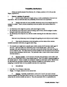
Graph of Men’s and Women’s Heights

Men Women

140 145 150 155 160 165 170 175 180 185 190 195 200 Height in centimetres


Areas Under the Distribution • What is the proportion of women that are taller than 175 cm?

Need this area

140

145

150

155

160

165

170

175

180

185

190

195

200

Height in centimetres Barrow, Statistics for Economics, Accounting and Business Studies, 4th edition © Pearson Education Limited 2006

Areas Under the Distribution (cont.) • How many standard deviations is 175 above 166? • One standard deviation is 40.32 = 6.35, hence

175  166 z  1.42 6.35 • So 175 lies 1.42 standard deviations above the mean So 175 lies 1.42 standard deviations above the mean • How much of the Normal distribution lies beyond 1.42 s.d’s above the mean? Use tables...


Table A2 The Standard Normal Distribution z

0.00

0.01

0.02

0.03

0.04

0.05

00 0.0

0 5000 0.5000

0 4960 0.4960

0 4920 0.4920

0 4880 0.4880

0 4840 0.4840

0 4801 0.4801

0.1

0.4602

0.4562

0.4522

0.4483

0.4443

0.4404















1.3

0.0968

0.0951

0.0934

0.0918

0.0901

0.0885

1.4

0.0808

0.0793

0.0778

0.0764

0.0749

0.0735

1.5

0.0668

0.0655

0.0643

0.0630

0.0618

0.0606













…




Answer • •

7.78% of women are taller than 175 cm. To find the area in the tail of the distribution: To find the area in the tail of the distribution: 1. Calculate the z‐score, given the number of standard deviations b t between the mean and the desired height th d th d i d h i ht 2. Then look the z‐score up in tables to get a probability 3. Use rules of symmetry where appropriate


The Distribution of the Sample Mean • If samples of size n are randomly drawn from a Normally distributed population of mean  and variance population of mean and variance 2, the sample mean the sample mean is is distributed as



x ~ N  , 2 n



• E.g. if samples of 50 women are chosen, the sample mean is distributed

x ~ N 166, 40.32 50 

• note the very small standard error: (40.32/50)=0.897


The Distributions of x and of x • Note the distinction between

  x ~ N  ,  n  x ~ N  ,

and

2

2

• The former refers to the distribution of a typical member of the population and the latter to the distribution of the sample mean population, and the latter to the distribution of the sample mean • We usually refer to the square root of the variance of the sample mean as the standard error h d d of the sample mean, rather than the f h l h h h standard deviation Barrow, Statistics for Economics, Accounting and Business Studies, 4th edition © Pearson Education Limited 2006

Example • Wh What is the probability of drawing a sample of 50 women whose t i th b bilit f d i l f 50 h average height is > 168 cm?

168  166  2.23 z 40.32 50 – z = 2.23 cuts off 1.29% in the upper tail of the standard Normal d distribution, so there is only a probability of 1.29% of drawing a b h l b bl f fd sample with a mean > 168 cm • Q. what is probability of drawing a sample with a mean 25) the population does not have to be Normally distributed, the sample mean is (approximately) Normal whatever the shape of the population distribution • The The approximation gets better, the larger the sample size. 25 is a safe approximation gets better the larger the sample size 25 is a safe minimum to use


Distributions when Samples are Small: Di ib i h S l S ll Using the t g distribution • When: – The sample size is small (