Probability distributions in conservative energy

INSTITUTE OF PHYSICS PUBLISHING

JOURNAL OF PHYSICS: CONDENSED MATTER

J. Phys.: Condens. Matter 19 (2007) 065138 (18pp)

doi:10.1088/0953-8984/19/6/065138

Probability distributions in conservative energy exchange models of multiple interacting agents Nicola Scafetta1 and Bruce J West1,2 1 2

Department of Physics, Duke University, Durham, NC 27708, USA Mathematics Division, Army Research Office, Research Triangle Park, NC 27709, USA

Received 29 August 2006, in final form 26 October 2006 Published 22 January 2007 Online at stacks.iop.org/JPhysCM/19/065138 Abstract Herein we study energy exchange models of multiple interacting agents that conserve energy in each interaction. The models differ regarding the rules that regulate the energy exchange and boundary effects. We find a variety of stochastic behaviours that manifest energy equilibrium probability distributions of different types and interaction rules that yield not only the exponential distributions such as the familiar Maxwell–Boltzmann–Gibbs distribution of an elastically colliding ideal particle gas, but also uniform distributions, truncated exponential distributions, Gaussian distributions, Gamma distributions, inverse power law distributions, mixed exponential and inverse power law distributions, and evolving distributions. This wide variety of distributions should be of value in determining the underlying mechanisms generating the statistical properties of complex phenomena including those to be found in complex chemical reactions.

1. Introduction One purpose of statistical mechanics [1] is to derive the constitutive equations of thermodynamics from the underlying microscopic equations of motion for the individual particles in a liquid, solid or gas. To accomplish this ambitious purpose an intermediate description of the physical system involving probability distributions was introduced. In the 19th century such distributions were considered to be merely convenient devices for keeping track of the many particle behaviour in complex phenomena. However, these distributions have come to take on a reality of their own, often capturing the essential features of complex phenomena. A typical example of this new reality is the statistical distribution of particles in an ideal gas [1]. These particles collide elastically, and because it is not possible to realistically describe the entire system by following the individual particle trajectories, one instead focuses on the statistical properties of a large collection of such trajectories. The ensemble distribution function then takes on a life of its own and determines how the physical variable being 0953-8984/07/065138+18$30.00 © 2007 IOP Publishing Ltd

Printed in the UK

1

J. Phys.: Condens. Matter 19 (2007) 065138

N Scafetta and B J West

considered changes over time or over the members of the ensemble. In the ideal gas, for example, the distribution function keeps track of how kinetic energy is distributed among the constituents of the gas. In the elastic collisions of an ideal gas the total kinetic energy of the colliding bodies after collision is equal to their total kinetic energy before collision. This equality is possible only if there is no conversion of kinetic energy into other forms. However, the conservation of kinetic energy is indeed a particular case of the more general conservation of energy principle that states that the total amount of energy in a closed system remains constant. In physics the form of the probability distribution function encapsulates the various conservation laws which constrain the system’s dynamics. This strategy has proven so successful in describing equilibrium and near-equilibrium phenomena in the physical sciences that many of the ideas have been transplanted from statistical mechanics into the social sciences. Consequently, to broaden the interpretive context of our discussion we shall replace the physical notion of a ‘particle’ with the more generic term ‘agent’, and although we shall continue to use the term ‘energy’ its meaning is that of anything two agents might exchange according to an interaction constrained by a conservation law. One such application that will be in the background of much of what is discussed herein is econophysics [2–6]. Econophysics can be considered a branch of the mathematical theory of complexity, and is closely linked to information theory, theories which were developed by physicists such as Shannon [7] and Gell-Mann [8], respectively. The rationale behind this philosophy is that physical models reflect economic phenomena because such phenomena are indeed the macroscopic result of the interactions of many agents on a microcosmic level; thus they are a particular kind of physical phenomena. Currently there are several fields and tools from physics that are being used in econophysics such as fluid dynamics, quantum mechanics, and the path integral formulation of statistical mechanics. The term ‘econophysics’ was coined by Stanley [4] in the mid 1990s, to describe the large number of papers written by physicists on the problems of (stock) markets [9], and first appeared in a conference on statistical physics in Calcutta in 1995 and its following publications. However, if for ‘econophysics’ we decide to denote a general application of physics concepts and methodologies to economics, we can consider the works of Léon Walras (1834–1910) [10] and Vilfredo Pareto (1848–1923) [11, 12] to be the initiators of the field. As historians in the science of economics [13] acknowledge, Elements of Pure Economics [10] led to Walras being considered the father of the general equilibrium theory of economics. Vilfredo Pareto (an Italian physicist, sociologist, economist and philosopher) further developed general equilibrium theory models for economics which were borrowed from physics and mechanical equilibrium. In particular, Pareto made several important contributions to the study of income distributions and to the analysis of individuals’ choices. He introduced the concept of Pareto efficiency and helped develop the field of microeconomics. Particularly famous is the so-called Pareto’s law concerning the distribution of income, a law that states that the income distribution, P(w), for the upper-class in societies presents an inverse power law tail of the type 1 P(w) ≈ μ , (1) w where μ is known as the Pareto index and w is the income level. Pareto found that for all societies he analysed the index μ has the value domain 1 < μ < 2. In the following sections, we study closed systems of interacting agents that are elastically exchanging energy, in the generic sense defined above. Energy is interpreted to be anything that can be exchanged and is conserved during the interaction: for example, total kinetic energy, the total mechanic energy, the mass, or even, as in the case of economic trading agents, money [14]. The only constraint in each interaction is that the amount of energy possessed by each agent is 2



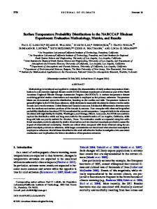
Figure 1. Elastic collision between two particles in which the total energy is conserved. The interaction causes only a transfer of an amount of energy εi j from one particle to the other.

non-negative (in analogy to the kinetic energy of a particle) because we assume this ‘energy’ to be something physical that can be exchanged between two agents and, naturally, an agent cannot give away what it does not possesses. Note that we avoid the notion of credit in this analysis. We will show that the common belief that random elastic collisions of a large number of ideal particles in an ideal gas can only yield the Maxwell–Boltzmann–Gibbs distribution [1] is not correct. In fact, the exponential Maxwell–Boltzmann–Gibbs distribution of colliding particles is based on the specific dynamical–statistical rules regulating the energy exchange during the collisions. However, through the various choices of energy exchange mechanisms determined by alternative properties and constraints we distinguish among a variety of complex systems characterized by different probability distribution functions of energy. Thus, we show that by changing these rules and also including some boundary effects, a variety of stochastic behaviours occur, manifesting energy conserving equilibrium probability distributions of different types. 2. Energy exchange models Our basic hypothesis is that all the energy contained in the initial state goes into the final state, which is to say there is no dissipation and the system is conservative. This means that if the initial energies of two particles are εi and ε j , respectively, and after the collision the energies are εi and ε j respectively, the following relation of conservation of energy is fulfilled:

εi + ε j = εi + εj ,

(2)

where, if we call εi j the amount of energy that transfers from the agent i to the agent j , we have

εi = εi + εi j εj = ε j − εi j .

(3) (4)

This simple idea is graphically represented in figure 1 and is presented at the risk of being pedantic in order to be clear about the changes in interaction being made in subsequent sections. Note that the amount of exchanged energy εi j can be positive (if agent i gains energy) or negative (if agent i loses energy). However, because we suppose that the energy of a single agent must always be non-negative, we assume that in each collision the amount of energy that 3



can be lost by an agent |εi j | cannot exceed the amount of the initial energy of the same agent. Thus, a collision between the agents i and j is characterized by the constraint

if εi < εi , if εj < ε j .

|εi j | εi , |εi j | ε j ,

(5)

or

(6)

The logical implication is that in a collision–interaction the extreme scenario would be that the final state is characterized by a situation in which one agent loses all its energy in favour of the other of the type:

εi = 0 εi

εj = εi + ε j ,

and

= εi + ε j

and

εj

= 0.

or

(7) (8)

Finally, the above roles regulating the interaction between two agents imply that given a large set of N colliding agents indicated by the index i = 1, 2, . . . , N , the total energy of the set is conserved in time, that is:

E=

N i=1

εi =

N

εi = const > 0.

(9)

i=1

Given the above general energy transfer role, the question we elect to answer is the following: given a set of elastically scattering agents, what is the system’s equilibrium probability distribution of energy, Peq (ε)? That is, if we assume, for example, that at the initial time t = 0 the energy is equally distributed among the N agents, εi (t = 0) = E/N for i = 1, 2, . . . , N , what is the form of Peq (ε) after a large number of collisions have occurred? It is evident that such an equilibrium distribution will depend on the particular rule regulating the amount and the direction of energy exchange εi j that is transferred from agent i to agent j in each collision. For example, it is evident that if for each collision we assume that there is always a null transfer of energy, εi j = 0, the equilibrium distribution would be equal to the initial distribution whatever it is, Peq (ε) = Pt=0 (ε), because in this case εi = εi for all i = 1, 2, . . . , N . It should be stressed that for the equilibrium probability distribution of energy, Peq (ε), we intend the most probable way of distributing the agents among various allowed energy states subject to the common constraints of a fixed number of agents, fixed total energy, and the additional particular constraints regulating the energy exchange mechanism itself. It is important to emphasize this maximal likelihood principle because it is always possible to realize that stochastic systems, which we study, might occasionally assume any possible configuration. For example, it is possible to argue that given a gas of colliding particles in a room if we wait a sufficiently long time it is possible to obtain a situation in which all the particles have equal energy, or all available energy is transferred to a single particle and all the other particles fall on the ground, or again that all the particles might occupy the left side of the room leaving the right side of the room completely empty. Of course, these situations are conceptually possible and statistically they could occur, but the probability of their realization is extremely small, and thus these unlikely situations will not be part of an equilibrium state of the system. In subsequent sections we study different physical scenarios by simply modifying the role regulating the amount and direction of energy εi j that transfers from the agent i to the agent j in each collision. We proceed with analytical demonstrations and/or numerical computer simulations. 4



Figure 2. Unconstrained random energy exchange models. The equilibrium distribution is an exponential function of the type of equation (13), Peq (ε) = β e−βε . We have used N = 10 000 particles with energy εi (t = 0) = E/N = 1/β and Peq (ε) is evaluated after 100 000 000 random collisions. We have used three different initial average energy values per particle: εi (t = 0) = 2; εi (t = 0) = 1; εi (t = 0) = 0.5. Note that the larger the energy, the wider the equilibrium distribution.

3. The simplest random energy exchange models and the Maxwell–Boltzmann distribution The most familiar and simplest kind of elastic scattering is the one characterized by pure unconstrained random exchange of energy among a set of agents such as the exchange of kinetic energy among the particles of an ideal gas [1]. For pure unconstrained random exchange of energy we intend that in each interaction between two agents the total available energy εi + ε j mixes and then randomly splits between the two agents with an equal probability for both agents to increase or lose energy. Formally this definition of elasticity means that the energy separates as

εi = εi + εi j εj = ε j − εi j

(10)

εi j = ξ(εi + ε j ) − εi ,

(12)

(11)

where 0 ξ 1 is a random number with uniform distribution that changes at each interaction. As is well know, this elastic scattering property yields the well-known Maxwell– Boltzmann distribution of energy, where the equilibrium distribution is given by an exponential function of the type

Peq (ε) ∝ e−βε ,

(13)

where β is an opportune constant that depends on the total energy E of the system. In figure 2 we show a few equilibrium distributions Peq (ε) for three computer experiments of unconstrained random elastic scattering obtained by assuming a set of N agents having at the beginning the same energy and letting them randomly interact for a sufficient amount of time such that the distribution of energy reaches an almost invariant form that is interpreted as representative of the most probable configuration of the system, the equilibrium form of the system. Note that the exponential-function form of the equilibrium distribution, a form that 5



is strongly asymmetric with a fast decay for large ε , can be expected because by adopting the above mechanism the collision does not have any memory of the past energy of the agents. Very energetic agents are severely disadvantaged by this mechanism because they always have a high probability of losing a significant amount of energy in any collision. Thus, the probability of finding energetic agents is expected to decay very quickly, according to a distribution having an exponential tail. The simulations in this study will always be carried out according to the above computational dynamical perspective. So, we deduce the equilibrium probability distribution of energy by simply letting N agents exchange energy for a sufficient amount of time according to equations (10) and (11) and to an additional specific condition describing the property of the exchange interaction such as the one expressed by equation (12). In this way our simulation actually simulates the natural process under study. However, in this particular case, which is the simplest meaningful one that can be thought of, we observe that this energy exchange process can be easily proven to be characterized by the probability distribution function in equation (13) by means of a simple statistical argument. In general, a statistical computation would be much more difficult if an exchanging rule different from equation (12) were adopted. In fact, we observe that the above process expressed by equations (10)–(12) is equivalent to a scenario where the N agents are arranged in a set of r distinguishable sub-states or microstates characterized by a given energy εz and each contains a given number of particles n z with z = 1, 2, . . . , r . No additional condition is required because the exchange rule expressed by equation (12) implies that the process is regulated only by the two basic system constraints we suppose for these models: r N= n z = const (14) z=1

E=

r

n z εz = const.

(15)

z=1

Thus, the most probable energy configuration can be easily estimated with simple statistical calculation. In fact, the number of possible random arrangements may be computed from the relation N! . W = (16) n 1 !n 2 ! · · · nr ! The equilibrium distribution Peq (ε) is the one that maximizes the number of arrangements W because this configuration is the most probable. To calculate Peq (ε) first we use the Stirling approximation formula for factorials, and obtain r r log(W ) = N log(N) − N − n z log(n z ) + nr . (17) z=1

z=1

Then, log(W ) can be maximized by considering the above two system constraints using the Lagrange multipliers α and β and imposing that the variation in the logarithm of the number of microstates is an extremum, that is: r r d log(W ) − α dn z − β ε z dn r = 0. (18) z=1

z=1

r

By using (17) we obtain d log(W ) = − z=1 log(n z ) dn z , and equation (18) becomes r (− log(n z ) − α − βεz ) dn z = 0. z=1

6

(19)



Thus, the number of particles in the state z in terms of the energy of the state and two Lagrange multipliers is given by

n z = e−α e−βεz . The constant α can be easily calculated by using the restriction

n z = N r

−βεz

e

z=1

e−βεz

.

r z=1

(20)

n z = N , to obtain (21)

Thus, the equilibrium probability Peq (ε) has an exponential form of the kind nε ∝ e−βε . Peq (ε) = (22) N In the particular case of thermodynamic equilibrium system such as a gas of scattering particles it is well known that β = 1/kT , with k being the Boltzmann constant and T being the temperature of the system [1]. The quantity kT is a measure of the average energy per particle E/N of the system. 4. Anomalous random energy exchange models In the following subsections we discuss different elastic models characterized by an anomalous random energy exchange mechanism. We show that when the collisions are regulated by anomalous rules that constrain the energy exchange and introduce boundary effects, they produce a kind of long-term memory effect on the agents. For example, in the simple unconstrained model studied in the previous section an agent loses any memory of its past at each collision. Instead, in the following cases it will not be so because the additional exchange constraints force the agents to retain memory of their past condition. This memory generates a stress inside the system that has the result of shaping the energy equilibrium probability distributions in a variety of forms different from the Maxwell–Boltzmann distribution, such as uniform distributions, truncated exponential distributions, Gaussian distributions, Gamma distributions, inverse power law distributions, mixed exponential and inverse power law distributions, and evolving distributions. 4.1. Models with energy saving: fixed percentage A simple variation of the unconstrained random elastic scattering model is one in which the agents before interacting save a fraction of their energy [15]. This means that not the entire amount of their energy but only a fraction λ of it is available for exchange. Thus, in each interaction between two agents the energy λ(εi + ε j ) mixes and then randomly splits between the two agents with an equal probability for both agents to increase or lose energy according to the equations


(23)

εi j = (1 − λ)[ξ(εi + ε j ) − εi ],

(25)

(24)

where 0 ξ 1 is a random number with uniform distribution that changes at each interaction and 0 λ 1 is a fixed saving fraction value. Of course, for λ = 0 this case reduces to an unconstrained random elastic scattering model discussed in the previous subsection. Again, the amount of energy available is randomly split between the two agents. Figure 3 shows the equilibrium distribution Peq (ε) for a few computer experiments for four values of the parameter λ between zero and one. For a vanishing value of the parameter λ = 0, 7



Figure 3. Models with energy saving: fixed percentage. The equilibrium distribution has a form that evolves from an exponential distribution for λ = 0 to a form that resembles a Gaussian distribution for λ approaching to 1. Observe that the for λ → 1 the maximum of the distribution approaches the value ε = 1 which in these simulations represents the average energy values per particle. We have averaged ten different realization by using for each of them N = 10 000 particles with energy εi (t = 0) = E/N = 1 and Peq (ε) is evaluated after 100 000 000 random collisions.

Peq (ε) converges to an exponential-like distribution, as expected. For a non-vanishing value of λ the equilibrium distribution Peq (ε) assumes a not-well-determined asymmetric-function form that converges to a Gaussian-like distribution for λ approaching the value 1. The reason for this convergence to a Gaussian-like distribution can be explained by observing that for λ → 1 the amount of energy that a particle can receive or lose in each collision is almost always a very small fraction of the energy available in each collision. These kinds of interaction conserve a strong memory of the past energy of the agents because the collisions will not drastically modify the energy of the interacting agents. This makes the process symmetric and the temporal evolution of the energy of each agent resemble a kind of random walk. Thus, using the central limit theorem the distribution will be a symmetric Gaussian distribution centred on the average energy value. 4.2. Models with energy saving: individual random percentage The scattering with an individual random percentage energy saving model [15] assumes that the energy saving percentage depends on the agent. In each interaction some agents will have little propensity for saving energy while others will save most of their energy. Herein, we generalize the model originally presented in [15] and assume that the agent i saves the percentage 0 λαi 1 of its own energy before each interaction. The saving percentage for each agent does not change in time and the set of {λi } is uniformly distributed in the interval [0 : 1]. The exponent α > 0 (which in [15] is α = 1) is supposed to be constant for all agents during all process and it is used to vary the distribution of percentage saving values {λαi }: for α = 1 saving percentage values are uniformly distributed; for 0 < α < 1 most agents will save energy in each interaction; for α > 1 most agents will share a large amount of their energy in each interaction. 8



Figure 4. Models with energy saving: individual random percentage. These equilibrium distributions show inverse power law tails of the type Peq (ε) ∝ ε −β with β ≈ 2. For α < 1 there appears a two class separation among agents with a small class characterized with high energy value, which follows an inverse power law tail distribution, and a class containing all other agents with a medium–low energy value, which follows a more exponential-like distribution. The value ε = 1 represents the average energy value per particle. We have used N = 100 000 agents with energy εi (t = 0) = 1 and Peq (ε) is evaluated after 100 000 000 random collisions. (In the figure the curves are vertically shifted for better comparison.)

In each interaction, again we suppose that the amount of energy available is randomly split between the two agents. Thus, with λαi and λαj the saving percentage of the two agents, the equations describing the interaction are

εi = εi + εi j

(26)

εj

(27)

= ε j − εi j εi j = (ξ − 1)(1 − λαi )εi + ξ(1 − λαj )ε j ,

(28)

where 0 ξ 1 is a random number with uniform distribution that changes at each interaction and 0 λi 1 for i = 1, 2, . . . , N are a set of random values uniformly distributed in [0 : 1] that remain fixed for each agent. Figure 4 shows three computer simulations with α = 0.01, α = 1 and α = 100. These equilibrium distributions show inverse power law tails of the type Peq (ε) ∝ ε −β with β ≈ 2. For α = 0.01 it is evident that the agents divide in two classes: a small class characterized with high energy value, which follows an inverse power law tail distribution, and a class containing all other agents with a medium–low energy value, which follows a more exponential-like distribution. The rationale for getting wide distributions with slowly decaying tails rests on the fact that with an individual random percentage energy saving mechanism a certain number of agents will save most of their own energy while others will share most of it in each interaction. Thus, the agents that share a small percentage of their energy will likely absorb a large amount of energy from the less energetic agents with which they interact. For α → 0 the great majority of agents will share almost all of their own energy in each interaction, as in the case of unconstrained random elastic scattering discussed above. Because the latter mechanism will be adopted by the majority of agents, and the cases when these agents 9



interact with one of the few very energetic agent are rare, the equilibrium distribution Peq (ε) for medium–low energy will resemble the exponential form of the Maxwell–Boltzmann–Gibbs distribution. For α 1 instead, most of the agents will save a large amount of their own energy at each interaction. Thus, the simulation shows an equilibrium distribution Peq (ε) that a medium–low energy will resemble a Gaussian distribution, as we have seen above to happen for a scattering with a high fixed percentage energy saving model, but there will still be a small but significant number of agents which collect a large amount of energy. These few agents are responsible for the inverse power law tail of the equilibrium distribution. Note that in this model the power law tail of the equilibrium distribution is indeed produced by that small number of objects which are characterized by a saving percentage value approaching the value of 1. By repeating the simulation with λαi distributed in the interval [0 : 0.9], the power law vanishes and the equilibrium distribution looks like those obtained with a scattering with a fixed percentage energy saving discussed in the previous subsection with a function form that resembles a gamma distribution for α = 1. If the saving percentage coefficients are not constant for each agent but randomly change in time the inverse power law tail again vanishes.

4.3. Models with fixed amount of energy exchange In the previous models we have hypothesized that the amount of energy εi j that transfers from one agent to the other might be a fraction of the sum of the energy of both interacting agents. Herein, we assume models in which in each interaction only a fixed small amount of energy η can transfer from one agent to another, with the only constraint being that the energy of each agent remains non-negative (see also [16, 17]). Without losing generality we can assume that the energy of each agent is an integer multiple k 1 of η: εk = kη. The first model assumes that the energy transfer in each interaction might favour either of the two agents, so the direction of the energy exchange is independent of the relative energy of the two agents. Thus, this mechanism is described by the following equations:

εi = εi + εi j

(29)

εj

(30)

= ε j − εi j εi j = η,

(31)

where η is a fixed small amount of energy. However, because the energy of an agent must be non-negative we impose the boundary condition that in an interaction an agent with ε = 0 can only absorb an amount η of energy from another agent with ε η, or not exchange any energy at all. Figure 5 shows how the probability distribution P(ε, t) of this model evolves in time. We suppose 100 000 agents that randomly interact by randomly exchanging a fixed amount of energy equal to η = 0.05 and that each agent has an initial energy of ε = 1. We plot P(ε, t) after one million interactions, after ten million interactions and one hundred million interactions. The figure shows that the distribution function has an interesting transformation when a certain number of agents hit the boundary at ε = 0. Before that the boundary at ε = 0 is met by the agents, the distribution is essentially Gaussian, or better a binomial distribution centred in ε = 1 because the agents’ energy undergo to a diffusive-like process equivalent to a random walk process with constant random jumps of length η. Thus, the probability distribution evolves 10



Figure 5. Models with fixed amount of energy exchange and a boundary condition at ε = 0. The probability distribution evolves from a Gaussian distribution (before contact with the boundary at ε = 0) to an exponential distribution of the type Peq (ε) = e−ε at equilibrium. The figure shows two realizations using N = 100 000 agents with energy εi (t = 0) = 1, and Peq (ε) is evaluated after 1000 000, 10 000 000 and 100 000 000 random collisions, respectively.

in time approximately as

(ε − 1)2 1 . P(ε, t) = √ exp − 2(ηt)2 2πηt

(32)

Once the boundary is encountered, a certain number of agents will condense on it and the symmetry of the process is broken because one half of the interactions these agents with energy ε = 0 have with the other agents will not have any effect. After a period of transition the energy distribution converges to an equilibrium distribution that decays exponentially:

Peq (ε) = e−ε .

(33)

The above model assumes that the system has a single lower boundary at ε = 0, while the high boundary is left open. However, it is possible to imagine a system with two finite boundary conditions such that the energy of any agent is within the limit 0 ε β,

(34)

where β indicates the upper boundary limit. Thus, as for the lower limit, if an agent has energy ε = β in an interaction with a less energetic agent it can release an amount η of energy or will not exchange anything. Figure 6 shows the equilibrium distribution Peq (ε) for a few computer simulations using the same lower boundary at ε = 0 and four different upper boundaries: β = 2; β = 2.5; β = 3 and β = 4. All simulations have been carried out assuming that all agents have initial energy ε(t = 0) = 1. Figure 6 shows that the equilibrium distribution Peq (ε) for β = 2 is a uniform distribution: Peq (ε) = 0.5. This can be explained by observing that the system is perfectly symmetric because the average energy for each agent is ε = 1. For β > 2 the equilibrium distribution Peq (ε) assumes an exponential form of the type

Peq (ε) =

g(β) e−g(β)ε , 1 − e−g(β)β

(35) 11



Figure 6. Models with fixed amounts of energy exchange and two boundary conditions: one at ε = 0 and the other ε = β > 2. The equilibrium distribution has a truncated exponential-function form of the type Peq (ε) ∝ e−g(β)ε , with g(β = 2) = 0 and limβ→∞ g(β) = 1. The figure shows two realizations using N = 100 000 agents with energy εi (t = 0) = 1, and Peq (ε) is evaluated after 300 000 000 random collisions, respectively.

where the function g(β) is monotonically increasing in β and satisfies the limit conditions

g(2) = 0

and

lim g(β) = 1.

β→∞

(36)

The case 1 < β < 2 can be easily obtained by using the symmetric properties of the system, and the equilibrium distribution Peq (ε) assumes an exponential form of the type

g(β) eg(β)ε , (37) −1 with the same function g(β). Two additional elementary models would constrain the direction of the energy transfer: (a) the energy can transfer only from a less energetic agent to a more energetic agent; (b) the energy can transfer only from a more energetic agent to a less energetic agent. If one thinks in terms of the transfer of wealth during a trade rather than the transfer of energy during a collision, certain social implications suggest themselves. In the former case evidently at equilibrium all energy is condensed into a single agent while all other agents have zero energy. Thus, the distribution will converge in time to a Dirac delta centred in zero, Peq (ε) → 2δ(ε), (the ‘2’ is because the distribution is defined for ε 0). In the latter case evidently at equilibrium all agents have the same energy. Certain economic theories also conclude that all wealth will wind up in the hands of the very few, leaving the rest of humanity to starve. Peq (ε) =

eg(β)β

4.4. Models with energy exchange bounded to the less energetic of the two agents In the previous models we have hypothesized that the amount of energy εi j that transfers from one agent to the other is related to the energy of both interacting agents. Herein we analyse a set of energy exchange models in which εi j is related only to energy of one of the two agents (see also [18, 19]). Because the energy of the agents has to be always non-negative, the simplest 12



Figure 7. Models with energy exchange bounded to the less energetic of the two agents. The equilibrium distribution is not stable and in time all energy is absorbed by a single agent. The distribution approaches an inverse power law function of the type Peq (ε) = 1/ε . The figure shows two realizations using N = 100 000 agents with energy εi (t = 0) = 1, and Peq (ε) is evaluated after 1000 000 and 10 000 000 random collisions, respectively.

of these models must be of the type


(38)

εi j = (2ξ − 1) min[εi , ε j ],

(40)

(39)

where 0 ξ 1 is a random number with uniform distribution that changes at each interaction. The above relation implies that in each interaction the less energetic trader might at most lose or gain an amount of energy equal to its own energy. It is evident that in such an interaction although both agents have the same probability of losing or gaining energy, the less energetic agent always runs a higher risk because the latter might lose a fraction of its energy while the former, if it loses energy, will always lose a smaller fraction of its own energy. Moreover, if in an interaction a less energetic agent loses an amount of its own energy, it will be less likely that this agent will gain an equal amount of energy in the following interaction. In fact, the decrease of its energy in the first interaction has also decreased the potential amount of energy that can be exchanged in subsequent interactions. This mechanism, which is essentially equivalent to the gambler’s ruin problem [20], does not lead to a stable equilibrium distribution of energy because this distribution becomes wider and wider in time. In fact, the most energetic agent continues to absorb energy from all the other agents and its energy approaches the total energy of the system while all other agents continue to lose energy and their energy approaches zero. However, this evolving distribution approaches an inverse power law distribution of the type

Peq (ε) =

1 , ε

(41)

as figure 7 shows. 13



In fact, the above process is almost equivalent to a multiplicative stochastic process where the energy of an agent evolves as dε i = φ(t)εi , (42) dt where −1 < φ(t) < 1 is a random number that is delta correlated in time. The above equation yields the Fokker–Planck equation for the evolution of the probability density of energy ∂(ε P) ∂P ∂ ε , (43) = ∂t ∂ε ∂ε which has equation (41) as the solution at equilibrium: ∂t∂ P = 0. Note that the above is only an approximation of the energy exchange model herein analysed because the multiplicative stochastic process described in equation (42) does not conserve the total energy of the system. However, without losing generality it can be hypothesized to periodically normalize the energy of the total system to force it to have a constant value. 4.5. Energy exchange oriented and bounded to the less energetic of the two agents: one parameter models In the above models we always assume that the two interacting agents have the same chance of gaining or losing energy. We simply changed the rules about the amount of energy εi j that could transfer from one agent to another. However, there is another set of models in which one of the two agents is favoured to gain energy in an interaction. This happens when the probability that an agent i will gain net energy is, for example, dependent on some function of the energies εi and εi (see also [18, 19, 21]). Two possible models are possible: the efficiency of gain energy increases or decreases with the energy. In the former case, the agent with higher energy will more likely absorb energy from an less energetic agent. In the latter case, the agent with lower energy will more likely absorb energy from a more energetic agent. In the former case all energy tends to be absorbed by a single agent that becomes more and more energetic. The latter case, instead, yields an interesting equilibrium distribution in cases when, in the absence of such a statistical bias that favours the less energetic of the two interacting agents, the mechanism favours only one agent. For example, let us adopt the multiplicative stochastic process studied in the previous subsection corrected with a simple mechanism that the less energetic of the two interacting agents, which we refer to as agent i , is more likely to absorb energy according to a probability bias function Pβ (i, j ) > 0.5 if εi < ε j . (44) Thus, in a simple model the equations describing the energy transfer interaction are εi = εi + σ εi j (45)

εj = ε j − σ εi j (46) εi j = ξ min[εi , ε j ], (47) where 0 ξ 1 is a random number with uniform distribution that changes at each interaction, with a probability bias function that, for example, might resemble a Planck distribution of the type 1 0. 5, Pβ (σ = 1) = with εi ε j , (48) ε 1 + exp(−β[ ij − 1]) Pβ (σ = −1) = 1 − 14

1 0. 5, ε 1 + exp(−β[ ij − 1])

with εi ε j ,

(49)



Figure 8. Energy exchange oriented and bounded to the less energetic of the two agents: one parameter models. The parameter β > 0 measures the strength of bias toward the less energetic of the two interacting agents. For β 1 the equilibrium distribution Peq (ε) approaches an inverse power law function. For larger values of β , Peq (ε) approaches a non-monotonic distribution with an exponential tail. Computer realizations using N = 100 000 agents with energy εi (t = 0) = 1, and Peq (ε) is evaluated after 20 000 000 random collisions.

where the parameter β 0 measures the strength of the statistical bias toward the less energetic of the two agents. So, if β = 0, Pβ (σ = 1) = Pβ (σ = −1) = 0.5, and the case reduces to the multiplicative stochastic process studied in the previous subsection. Instead, if β > 0 the less energetic of the two agents has a higher chance to absorb energy from the other agent because 0.5 < Pβ (σ = 1) < 1. This probability increases with the energy gap between the two agents, εi ε j , while for two agents with the same energy εi = ε j , there is no bias, and the bias probability again is Pβ (σ = 1) = Pβ (σ = −1) = 0.5. Figures 8 and 9 show a few computer simulations. For β 1 the equilibrium distribution Peq (ε) approaches an inverse power law function. For larger values of β , Peq (ε) approaches a non-monotonic distribution with an exponential tail that decays more quickly as β increases. Figure 9 suggests that these equilibrium probability distributions are well fitted with Gamma distributions. Also, for β → ∞, that corresponds to the case in which the less energetic of the two agents always absorbs energy from the more energetic one, the equilibrium distribution rapidly converges to a characteristic Gamma-like probability density function. 4.6. Energy exchange oriented and bounded to the less energetic of the two agents: two parameter models In the previous subsection we have adopted a model that depended only on one parameter β > 0. Moreover, we chose a probability bias function Pβ (i, j ) of the type of a Plancklike function and assumed that the transfer energy amount could not exceed the amount of the less energetic of the two agents. This is not a necessary condition for getting a Gamma-like equilibrium density function. To prove this herein we adopt a different model that adopts a similar philosophy but with a different probability bias function and with a different definition of the amount of energy transfer. The amount of energy that can be transferred from one agent to the other depends on an additional parameter α that is a measure of the fraction of the energy 15



Figure 9. Models as in figure 8. The histograms are fitted with appropriate Gamma functions, (ε), of the type Peq (ε) = a(ε − b)c exp(−dε), with a , b, c and d appropriate fitting parameters. The curve for ‘Beta = inf’ corresponds to the case β → ∞. The case β → ∞ corresponds to the case in which the less energetic of the two agents always absorbs energy from the more energetic one.

of the less energetic of the two agents might be exchanged in each interaction. For generality we assume that the less energetic of the two agents might occasionally absorb or lose an amount of energy that might be even slightly larger than its actual energy, but this amount should always be comparable with its own energy. Thus, in a simple model [18, 19] the equations are

εi = εi + εi j

(50)

εj

(51)

= ε j − εi j ,

where εi j might be positive or negative and, for example is distributed according to the following probability density function: i j )2 (εi j − ε 1 , Pα,β (εi j ) = exp − (52) 2σi2j 2πσ 2 ij

where

σi j = α min(εi , ε j ) (53) i j = β ε j − εi σi j ε (54) ε j + εi with α > 0 and β > 0. Thus, if εi = ε j the two agents have the same probability to gain or lose energy. However, if εi < ε j the agent i has a better chance to absorb energy from the agent j . The parameter α measures the statistical width of the fraction of energy involved in each transaction, and the parameter β measures the strength of the statistical bias favouring the less energetic of the two traders. Figures 10 and 11 show a few computer simulation examples. By keeping β constant and increasing α the Gamma-like equilibrium probability distributions become wider. This is also obtained by keeping α constant and decreasing β . This can be easily explained by observing that with small α and large β it is more difficult for the low energetic agent to further lose energy and for very energetic agents to further absorb energy. 16



Figure 10. Energy exchange oriented and bounded to the less energetic of the two agents: two parameter models. The parameter α > 0 measures the width of distribution of the transfer energy amount relative to the lower energy amount between the two agents, while β > 0 measures the strength of bias toward the less energetic of the two interacting agents. By keeping β constant and increasing α the Gamma-like equilibrium probability distributions become wider. Computer realizations using N = 100 000 agents with energy εi (t = 0) = 1, and Peq (ε) is evaluated after 20 000 000 random collisions.

Figure 11. Models as in figure 10. By keeping α constant and decreasing β the Gamma-like equilibrium probability distributions become wider.

5. Conclusion Herein we have studied several energy exchange models of multiple interacting agents that conserve energy in each interaction, such as occurs in the elastic collision of particles. We have simply changed the rules that regulate the amount and the direction of energy exchange, and in some cases we have included some boundary effects that limit the amount of energy that a single agent can have. 17



We have shown that contrary to traditional wisdom the well-known exponential Maxwell– Boltzmann–Gibbs distribution of energy for elastically colliding particles is not the only possible outcome of elastic interactions. In fact, the exponential Maxwell–Boltzmann–Gibbs distribution of energy depends crucially on the hypothesis that during a collision the energy of the two agents mixes and then randomly splits between the two particles. We have found that a different hypothesis regarding the amount and the direction of energy exchange gives rise to a variety of complex stochastic behaviours that manifest energy equilibrium probability distributions of different types. In addition to the familiar Maxwell– Boltzmann–Gibbs distributions, we also found uniform distributions, truncated exponential distributions, Gaussian distributions, Gamma distributions, inverse power law distributions, mixed exponential and inverse power law distributions, and evolving distributions that do not manifest a stable equilibrium. We expect that many if not all these statistical distributions are to be found among complex chemical reactions. Acknowledgment N Scafetta thanks the Army Research Office for support of this research. References [1] Pathria R K 2001 Statistical Mechanics (Oxford: Butterworth-Heinemann) [2] Farjoun E and Machover M 1983 Laws of Chaos; A Probabilistic Approach to Political Economy (London: Verso) [3] Mirowski P 1989 More Heat than Light—Economics as Social Physics, Physics as Nature’s Economics (Cambridge: Cambridge University Press) [4] Mantegna R M and Stanley H E 1999 An Introduction to Econophysics: Correlations and Complexity in Finance (Cambridge: Cambridge University Press) [5] McCauley J 2004 Dynamics of Markets, Econophysics and Finance (Cambridge: Cambridge University Press) [6] Chatterjee A, Yarlagadda S and Chakrabarti B K 2005 Econophysics of Wealth Distributions (Milan: SpringerVerlag Italia) [7] Shannon C E 1948 A mathematical theory of communication Bell Syst. Tech. J. 27 379–423 Shannon C E 1948 Bell Syst. Tech. J. 27 623–56 [8] Gell-Mann M 1994 The Quark and the Jaguar: Adventures in the Simple and the Complex (New York: Freeman) [9] Sornette D 2004 Why Stock Markets Crash: Critical Events in Complex Financial Systems (Princeton, NJ: Princeton University Press) ´ ements d’économie Politique Pure, ou Théorie de la Richesse Sociale (1899, 4th edn, 1926, [10] Walras L 1874 El´ revised edn) Walras L 1954 Elements of Pure Economics, or The Theory of Social Wealth (Engl. Transl.) [11] Pareto V 1906 Manuale di Economia Politica (Italian (1909, French Transl.)) Pareto V 1971 Manual of Political Economy (Engl. Transl.) [12] Pareto V 1911 Economie mathèmatique Encyclopedie des Sciences Mathematiques (Gauthier-Villars) [13] Ingrao B and Israel G 1990 The Invisible Hand—Economic Equilibrium in the History of Science (Cambridge, MA: MIT Press) [14] Dragulescu A and Yakovenko V M 2000 Statistical mechanics of money Eur. Phys. J. B 17 723–9 [15] Chatterjee A, Chakrabarti B K and Manna S S 2004 Pareto law in a kinetic model of market with random saving propensity Physica A 335 155–63 [16] Feller W 1971 An Introduction to Probability Theory (New York: Wiley) [17] Ispolatov S, Krapivsky P L and Redner S 1998 Wealth distributions in asset exchange models Eur. Phys. J. B 2 267–76 [18] Scafetta N, Picozzi S and West B J 2004 An out-of-equilibrium model of the distributions of wealth? Quantitative Finance 4 353–64 [19] Scafetta N, Picozzi S and West B J 2004 A trade-investment model for distribution of wealth? Physica D 193 338–52 [20] Norris J R 1997 Markov Chains (Cambridge: Cambridge University Press) [21] Sinha S 2003 Stochastic maps, wealth distribution in random asset exchange models and the marginal utility of relative wealth Phys. Scr. T 106 59–64

18