Probability distribution function of the temperature increment in isotropic turbulence. Iwao Hosokawa. Unioer sity of Electro Co-mmunications,. Chofu, Tokyo 182 ...
PHYSICAL REVIEW E
VOLUME 49, NUMBER 6
Probability distribution
function of the temperature
Unioer sity
JUNE 1994
increment
in isotropic turbulence
Iwao Hosokawa of Electro Co-mmunications, Chofu, Tokyo 182, Japan (Received 4 October 1993)
The statistics of a temperature increment across a distance in the inertial range in isotropic turbulence is discussed on the basis of the Obukhov-Corrsin similarity, the extensive use of the Kolmogorov refined similarity hypothesis and the three-dimensional tetranomial Cantor set model for isotropic turbulence with a passive advected scalar. The result compares well with available experimental data. PACS number(s): 47.27. —i, 05.45.+b, 02. 50.—r
Although there are some models for isotropic turbulence in which the probability density function (PDF) of velocity increment across a distance in the inertial range in isotropic turbulence has been discussed in a reasonable way [1— 3], the PDF of a temperature increment advected in isotropic turbulence still seems to be diKcult to explain by such a simple model. In fact, Jensen, Paladin, and Vulpiani [4] tried a numerical approach using a joint shell model of the Navier-Stokes equation and the advected scalar equation, instead of extending the random P model for isotropic turbulence [5] they trust. Their result for the PDF of a temperature increment seems to be reasonable at least qualitatively, though missing a comparison with experiment. However, as such a shell model needs a considerable amount of computer work, a simpler model approach would be more convenient if it exists with enough reliability. On the other hand, a dynamical method was proposed by Sinai and Yakhot [6) to treat the PDF of temperature itself, and extended (with some assumptions) by Ching [7] to predict the PDF of a temperature increment between different times in Rayleigh-Benard convection. But in this method there is an unknown function (which is considered to depend on time separation 7), so that it should be searched empirically by some independent data. Therefore a simple calculation is reported here, which naturally arises from the multifractal model for isotropic turbulence associated with a passive advected scalar recently proposed by the author as the three-dimensional (3D) tetranomial Cantor set model [8]. It is already known that this explains temperature structure functions very well in comparison with the experiment of Antonia et al. [9]. We start by describing this model. Let us introduce joint intermittency exponents p(q, p), which implies joint scale similarity of energy dissipation rate e and temperature dissipation rate y (per mass), as
((e /«)'(X. /&t)')
= (r/&) ""'"'
= log&
(
o
y~z"p(y, z; A o
1063-651X/94/49(6)/4775(4)/$06. 00
)dy
p(y, z; A
') = A[b(y —B)b(z —D) + b(y —C)b(z —E)] +(1/2 —A) [b(y —B)b(z —I') +b(y —C)b(z —G)]
dz,
(2) 49
(3)
as a natural extension of the 3D binomial Cantor set model [10], in which A = 2 1 (we take here d = 3) and B, C = 1 + (2"~~ —1)'~' [p = y, (2, 0); tt = 0.2 is an accepted value]. From the consideration of temperature structure functions, the set of values A = 0.1556, D = 1.0669, E = 0.3576, F = 1.2, and G = 1.06 were previously recommended [8]. Joint generalized dimensions D(q, p) are related with t (q, p) as
p(q, p)
= (q —l)(p —l)D(q, p) + d(q + p —1).
Then generalized
dimensions
D(0, p) are given by setting
(4)
of temperature dissipation = 0 in the above proce-
q
dure. We can see them thus obtained &om our model in Fig. 1 in comparison with Jensen, Paladin, and Vulpiani's numerical result. Both are in agreement at p = 2, but elsewhere they deviate. In order to say which is better, however, we would need a comparison with data of accurate 3D direct numerical simulation, etc. [From the mathematical point of view, the following is worth not-
2.9 2.8 2.7 2.6
(1)
where a subscript means the scale, over a domain of which these quantities are averaged, and a domain of scale r should be included in that of scale I (& r) The angula. r brackets denote an ensemble average. If the joint PDF = z is known as p(y, z; r/l), we of e„/e~ = y and y„/yt — may write
y (q, p)
where A is l/r and d is spatial dimension. The 3D tetranomial Cantor set model is given by taking
D(0, p)
FIG. 1. Generalized dimensions of temperature dissipation rate.
The solid line shows the 3D tetranomial Cantor set model [8]. The circles with error bars are the result of computation by Jensen, Paladin, aud Vulpiaui [4] based on their joint shell model equation. R4775
1994 The American Physical Society
49
IWAO HOSOKAWA
R4776
ing. In case the requirement of our model that p(0. 1) = 0 has been only approximately fulfilled, a locally divergent behavior of D(0, p) can happen very near p = 1. This But behavior is solely due to such an approximation. this can be suppressed as much as we want by more accurately forcing the set of parameters to give p(0. 1) = 0. In fact, the behavior occurs in Fig. 1 in a negligibly slight region covering p = 1. However, the PDF of a temperature increment (described below) is entirely insensitive to such an adjustment. ] According to Obukhov [11] and Corrsin [12], we may
pz(2'„) =
ff
P[r/(rz&
z&e*
y
express the temperature
increment
„„x/3-x/6
as x/2
based on the dimensional argument, where e is a nondimensional variable but generally conditioned by r, and Here, let us apply extensively the refined similarity hypothesis (RSH) of Kolmogorov [13] and Obukhov and y4, as [14] in the form that v is independent of r, the first approximation. Then, if the PDF of e is given as P(v), the PDF of is written as
c„,
y„.
s„,
T„
&
)]/(rz& y
&
z
~
)p(y, z;r)dydz
(6)
is natural to restrict our treatment to such cases as these authors treated. We also note that the nearly Gaussian temperature PDF was recognized in a numerically simulated decaying isotropic turbulence with a passive scalar [21]. Our approach may be applicable to the soft turbulence regime of Rayleigh-Benard convection with Gaussian PDF of temperature, but it is a future problem to be taken up. [We avoid all the cases with the heating and cooling mechanism caused by an inserted (hot and cold) temperature boundary condition, such that there emerge wide, central turbulent regions with locally vanishing mean temperature gradients but having nonGaussian PDF's of temperature. Such cases are treated in Castaing et al. [16] and Ching and Tu [22]. The source of the exponential PDF of temperature there is plausibly explained by Castaing et al. as the intermittent aspiration events of the mixing zone near the boundary that obey a Poisson distribution. ] To proceed with the calculus, we need an expression of p(y, z;r) for arbitrary r. We adopt extensively the procedure relating p(y; r) to p(y; A ~) developed in the theory of the 3D binomial Cantor set model [10]. Then we may have
Here and hereafter r should read r/L (L is an integral scale). When r + 1, p(y, z; r) goes towards h(y —1)b(z— 1) and then ps(T„) P(T„).Although the theories of
~
Sinai and Yakhot [6] and Ching [7] do not necessarily support it, we assume here that ps(T„) for r near 1 is nearly Gaussian with zero mean for simplicity, just as well as the PDF of the velocity increment [1— 3], and then so is P(v). We note that Eswaran and Pope's direct numerical simulation [15] is in favor of this assumption. Of course, there have been several arguments that the PDF of temperature itself is non-Gaussian and has an exponential tail in the presence of mean (background) temperature gradient, since Castaing et al. [16] found that the PDF of temperature in Rayleigh-Benard convection was non-Gaussian for large Rayleigh numbers (that belong to the hard turbulence regime). Pumir, Shraiman, and Siggia [17] argued theo'r'etically the occurrence of the exponential tail in such a case, and Jayesh and Warhaft [18] and Gollub et aL [19] verified it experimentally. But we cannot overlook the parts of the experiments of Jayesh and Warhaft [18] and Thoroddsen and Van Atta [20] for grid generuted -turbulence, which showed that the PDF of temperature itself is nearly Gaussian in the absence of mean temperature gradient. Therefore it I
p(y,
z;r) =
ff
e
"r" "*~[ (
'~
d,
y;
ed)]
de de/[(yz) yz],
(7)
with
$(y, e;A
)
=
ff
e'~
~
zz"'
*~p(y, z;A z)dyde
lnB+zd lnD) P[ i(8
+ ei(8 1nC+e 1nE)] + (1/2
which is a joint characteristic function of lny and ln z, and (where 0 is assumed to be a natural number), we arrive at
(
. )
)
C
p)D
p/y(1/2
—ly
)
C
P)[ei(8 1nB+z 1nF)
0 = —lnr/ln ~l+ynCQ
C h(
+
i(8 lnC+m lnG)] j&
A. After double binomial expansion of Pn l
yyy)g(
ly — Dl— @— ly
m~0 — —yyy)
l, rn
Thus it is easy to obtain
ps(T„)= (2m)
~
)
llC~A" (1/2
—A)
"
)
t, fn
), Cl ll
/,
(8)
C exp[ —T„/(2S&1 )]/Sl, l
ly
(9)
PROBABILITY DISTRIBUTION FUNCTION OF THE.
49
..
R4777 TI. P(TI- l I
-20
-5
-10
20
lag10 I 3
Ph
10
lag10 I 3
FIG. 2. The PDF of the normalized temperature increment for r = 0.0108, the normalized shortest length in the inertial range for R& ——852. The squares are experimental values by Antonia et al. [9] and the solid line shows the present result.
FIG. 3. The PDF of the normalized temperature gradient for Rq —41 and 5. Thoroddsen and Van Atta's experiment [20] is shown by squares for R1 = 41 and triangles for Rz = 5, respectively. The solid lines show the present result for both cases.
with
™)
—1/6(DlEs —l+~gn —k —m) 1/2
pl/3(Bl+mgn —
(10)
It is not restrictive to assume that the variance of P(v)
T„
is unity, since we are interested in finally normalized by its root mean square, which is obtained from (10) as
(T2)1/2
rl/3[P(gy
+(1/2
—1/3D
+ Q —1/3E) P)(B / y'+ / l
G)]n/
In this theory ps(T„)does not depend on Reynolds number and Prandtl number, until r reaches either the Kolmogorov microscale g or the counterpart for the temperature field ge. Therefore it is suitable for the inertialconvective range in isotropic turbulence. In Fig. 2 we can see a ps(T„) compared with the experiment of Antonia et al. [9], which was performed for Rp = 852 (R~ is a Taylor-scale Reynolds number); here r is taken as the shortest scale in the inertial range they measured. Although the experimental result somewhat lacks symmetry, accordance seems to be good. The theory predicts in6ection points in the PDF at both sides for such a small r. This feature may remain problematic. At present, this tendency seems to be unavoidable so long as we adopt a 3D tetranomial Cantor set model which can derive reasonable temperature structure functions. In order to ensure this fact, however, a high precision in any device would be necessary since +10 the inBection points appear for the normalized with log1ops(T„) — 3; the points are further estranged downwards with less probability as r becomes smaller.
T„=
(
(T". )
=
)
n&l &"(1/2
—&)"
and therefore
aR&,
(»); —1&~3~l',l~
l, m
k
—374/3[/(g
").~An
We note here that the PDF of (normalized) temperature itself in the same experiment, which was shown together in Fig. 1 in [9], is nearly Gaussian, although it has some asymmetry. This justifies our assumption that P(v) is Gaussian, at least, to the first approximation. It is also interesting to compare the theory with the recent experiment of Thoroddsen and Van Atta [20], who showed the PDF of a temperature gradient for Rp —41 and 5 with the evidence of near-Gaussianity of the PDF of temperature itself in the absence of mean temperature gradient (as described above). For this purpose, we assume that the PDF of the normalized temperature gradient is equal to that of the normalized temperature increment for r = g. Hence the PDF can be calculated where a is 15 / according using the relation g = to Tennekes and Lumley [23]. The result is shown in Fig. 3. It is rather surprising that the agreement of theory and experiment is so good again, if we consider that we hardly have an inertial range in these cases. This suggests that such a scale similarity as assumed with (1) and its equivalent (4) holds for a broader range of r and Rp than expected. This is consistent with the fact revealed by Fig. 3 in [21,24] that the scaling law represented by generalized dimensions for energy dissipation in isotropic turbulence D(q, 0) [and so, probably, its extension D(q, p)] holds far beyond the inertial range. Also it has been assured by Chen [25] in forced isotropic turbulence that generalized dimensions are almost independent of Rp, even if it is much smaller than 100. We can calculate the kurtosis of the PDF by means of
—2/3D2
+g
2/3E2)
+ (1/2
p)(g
—2/3@2 — —2/sg2)]n
+g
(12)
T4
49
IWAO HOSOKAWA
R4778
T2
2
—
3 log~([A(B — 3 0. 2987
D +C
E )+(1/2 —A)(B
*F +C
G )]/[A(B
D+C
E)+(1/2 —A)(B
F+C
G)]
(13 t
If the real kurtosis
is different from this, either the model or the purely Gaussian form of P(v) may be doubted. The values of kurtosis of any curves in Figs. 2 and 3 were not pronounced in the papers [9,20]. But recently Thoroddsen and Van Atta [20] informed the author in a private communication that the estimated kurtosis for 41 and 5 in Fig. 3 were, respectively, 8.2 and 3.9, Rp — while the corresponding values based on (13) are, respectively, 8.6 and 3.4. Considering unavoidable experimental errors, the accordance seems to be very good. Although the estimated kurtosis in Fig. 2 is unavailable yet, the apparent similitude of theory and experiment is encouraging to the same degree as in Fig. 3. Just recently, Antonia and Zhu [26] measured the r dependence of kurtosis of temperature increment as well as velocity increment at the same time in turbulence in a circular jet for Bp = 250 and in an atmospheric turbulence for Rp —7600, and they obtained the r dependence with 0.3 in the inertial range for the average exponent of — both cases. This indicates that the exponent of (13) is
almost valid in the inertial range. [At the same time they obtained the r dependence of kurtosis of velocity 0.1 in the inerincrement with the exponent of about — tial range, which is within the currently accepted value, —0.09 —0.12 [27]. The 3D binomial Cantor set model, on which the present theory is based, predicts the ex0.0917 after a similar analytical calculation ponent as — using the ps(Eu, ) given in [3].] Thus it may be concluded that the present simple approach to the PDF of a temperature increment in isotropic turbulence expressed by (6) works considerably well to describe the average nature in some region of r covering the inertial range, insofar as the turbulent temperature field with a Gaussian PDF of temperature itself is treated. If a possible deviation &om Gaussianity of P(v) (depending on r, y, and z in principle) is taken into account from the more exact point of view which eventually goes oE the RSH, the theory would have a possibility of refinement and extension.
[1] R. Benzi, L. Biferale, G. Paladin, A. Vulpiani, and M. Vergassola, Phys. Rev. Lett. BT, 2299 (1991). [2] P. Kailasnath, K. R. Sreenivasan, and G. Stolovitzky,
Libchaber, S. Thome, X.-Z. Wu, S. Zaleski, and G. Zanetti, J. Fluid Mech. 204, 1 (1989). [17] A. Pumir, B. Shraiman, and E. D. Siggia, Phys. Rev.
Phys. Rev. Lett. 88, 2766 (1992). [3] I. Hosokawa, J. Phys. Soc. Jpn. 82, 10 (1993). [4] M. H. Jensen, G. Paladin, and A. Vulpiani, Phys. Rev. A 45, 7214 (1992). [5] R. Benzi, G. Paladin, G. Parisi, and A. Vulpiani, J. Phys. A 17, 3521 (1984). [6] Y. G. Sinai and V. Yakhot, Phys. Rev. Lett. 83, 1962
(1989). E. S. C. Ching, Phys. Rev. Lett. 70, 283 (1993). I. Hosokawa, Phys. Rev. A 43, 6735 (1991). [9] R. A. Antonia, E. J. Hopfinger, Y. Gagne, and F. Anselmet, Phys. Rev. A 30, 2704 (1984). [10] I. Hosokawa, Phys. Rev. Lett. BB, 1054 (1991). [7] [8]
[11] A. M. Obukhov, Izv. Akad. Nauk SSSR, Ser. Geogr. Geo6z. 18, 58 (1949). [12] S. Corrsin, J. Appl. Phys. 22, 469 (1951). [13] A. N. Kolmogorov, J. Fluid Mech. 13, 82 (1962). [14] A. M. Obukhov, J. Fluid Mech. 13, 77 (1962). [15] V. Eswaran and S. B. Pope, Phys. Fluids 31, 506 (1988). [16] B. Castaing, G. Gunaratne, F. Heslot, L. Kadanoff,
Lett. 88, 1984 (1991). [18] Jayesh and Z. Warhaft, Phys. Rev. Lett. BT, 3503 (1991). [19] J. P. Gollub, J. Clarke, M. Gharib, B. Lane, and O. N. Mesquita, Phys. Rev. Lett. BT, 3507 (1991). [20] S. T. Thoroddsen and C. W. Van Atta, J. Fluid Mech. 244, 547 (1992). [21] I. Hosokawa and K. Yamamoto, in Turbulence and Coherent Structures, edited by O. Metais and M. Lesieur (Kluwer Academic, Dordrecht, 1991), p. 177. [22] E. S. C. Ching and Y. Tu, Phys. Rev. E 49, 1278 (1994). [23] H. Tennekes and J. L. Lumley, A First Course in Tur bulence (MIT Press, Cambridge, MA, 1972), pp. 67 and
68. Hosokawa and K. Yamamoto, J. Phys. Soc. Jpn. 59, 401 (1990). [25] S. Chen (private communication). [26] R. A. Antonia and Y. Zhu (private communication). [27] Z. -S. She, S. Chen, G. Doolen, R. H. Kraichnan, and S. A. Orszag, Phys. Rev. Lett. TO, 3251 (1993).
[24]
I.