Perception & Psychophysics 2004, 66 (1), 104-118
Probability matching, accuracy maximization, and a test of the optimal classifier’s independence assumption in perceptual categorization W. TODD MADDOX University of Texas, Austin, Texas and COREY J. BOHIL University of Illinois at Urbana-Champaign, Champaign, Illinois Observers completed perceptual categorization tasks that included 25 base-rate/payoff conditions constructed from the factorial combination of five base-rate ratios (1:3, 1:2, 1:1, 2:1, and 3:1) with five payoff ratios (1:3, 1:2, 1:1, 2:1, and 3:1). This large database allowed an initial comparison of the competition between reward and accuracy maximization (COBRA) hypothesis with a competition between reward maximization and probability matching (COBRM) hypothesis, and an extensive and critical comparison of the flat-maxima hypothesis with the independence assumption of the optimal classifier. Model-based instantiations of the COBRA and COBRM hypotheses provided good accounts of the data, but there was a consistent advantage for the COBRM instantiation early in learning and for the COBRA instantiation later in learning. This pattern held in the present study and in a reanalysis of Bohil and Maddox (2003). Strong support was obtained for the flat-maxima hypothesis over the independence assumption, especially as the observers gained experience with the task. Model parameters indicated that observers’ reward-maximizing decision criterion rapidly approaches the optimal value and that more weight is placed on accuracy maximization in separate base-rate/payoff conditions than in simultaneous base-rate/payoff conditions. The superiority of the flat-maxima hypothesis suggests that violations of the independence assumption are to be expected, and are well captured by the flat-maxima hypothesis, with no need for any additional assumptions.
Categorization performance that maximizes long-run reward often requires the placement of a decision criterion along some relevant dimension. For example, an expedition doctor on a high-altitude trek through the Himalayas must decide whether a trekker’s poor coordination is a sign of cerebral edema or exhaustion, with a diagnosis of cerebral edema leading to an immediate retreat to a lower altitude. The location of the optimal decision criterion depends on the category base rates (i.e., the prior probability of each category) and the payoffs associated with correct responses. (The costs associated with incorrect responses also affect the location of the optimal decision criterion, but in the present study these were held fixed at zero and will not be discussed further.) Category base rates can differ across categorization situations. For example, at low altitude, cerebral edema has a low base-rate This research was supported in part by Grant 5 R01 MH59196 from the National Institute of Mental Health, National Institutes of Health. We thank three anonymous reviewers for helpful comments on an earlier version of this manuscript. Correspondence concerning this article should be addressed to W. T. Maddox, Department of Psychology, University of Texas, 1 University Station A8000, Austin, TX 78712 (e-mail:
[email protected]). Note—This article was accepted by the previous editorial team, headed by Neil Macmillan.
Copyright 2004 Psychonomic Society, Inc.
probability, but at high altitude the base rate increases. Because the base rate increases with altitude, the optimal strategy at high altitude is to lower the coordination decision criterion that leads to a diagnosis of edema. Lowering the coordination decision criterion in such a way maximizes reward and accuracy simultaneously. The payoffs associated with correct decisions can also differ. For example, the payoff associated with a correct “cerebral edema” decision is likely greater than the payoff associated with a correct “exhaustion” decision, since the former saves lives. Under these conditions, the doctor would be wise to lower the coordination criterion associated with a diagnosis of edema. In this case, lowering the coordination criterion maximizes reward but does not maximize accuracy. This tradeoff between reward and accuracy is of central importance to an understanding of categorization and decision-making behavior. Maddox and Dodd (2001) proposed a formal theory of decision criterion learning, and a model-based instantiation that incorporates this tradeoff by assuming that decision criterion placement results from a competition between reward and accuracy maximization (COBRA). The details will be outlined shortly, but for now suff ice it to say that COBRA assumes that the decision criterion used by the observer on any given trial is determined from a weighted combina-
104
MATCHING, MAXIMIZING, AND THE INDEPENDENCE ASSUMPTION tion of the observer’s estimate of the reward-maximizing decision criterion and the accuracy-maximizing decision criterion (see Equation 6 below). The observer’s estimate of the reward-maximizing decision criterion is determined according to the flat-maxima hypothesis. In short, the flat-maxima hypothesis assumes that the observer adjusts the estimate of the reward-maximizing decision criterion on the basis of the change in the rate of reward, with larger changes in rate being associated with faster, more nearly optimal decision criterion learning. The change in the rate of reward varies as a function of a number of important situational factors, such as category discriminability, base-rate/payoff ratio, magnitude of the payoff matrix entries, and whether base rates, payoffs, or both vary within a given situation. Maddox and Dodd’s hybrid model framework, which instantiates simultaneously the COBRA and flat-maxima hypotheses, has been successfully applied to decision criterion learning experiments in which each of these situational variables, as well as several others, was examined. For a review of this body of work, see Maddox (2002). The aim of the present study is twofold. Our first goal is to develop and test an alternative to the COBRA hypothesis. COBRA assumes that the decision criterion used by the observer on each trial is determined from a weighted average of the estimated reward-maximizing decision criterion (determined from the flat-maxima hypothesis) and the decision criterion that maximizes accuracy. The alternative assumes that there is a competition between reward maximization and probability matching (COBRM).1 The longstanding interest in the matching– maximizing dichotomy makes this an important issue (see, e.g., Ashby & Maddox, 1993; Estes, 1976; Herrnstein, 1961, 1970; Herrnstein & Heyman, 1979; Williams, 1988). We compare versions of the hybrid model that instantiate COBRA with versions that instantiate COBRM. To anticipate, we find support for both probability matching and accuracy maximization, but the results argue for a shift from probability matching early in learning toward accuracy maximization later in learning. Second, we replicate and extend a study by Bohil and Maddox (2003), who compared human decision criterion learning when base rates and payoffs were manipulated separately as opposed to simultaneously. Base rates and payoffs vary widely in real-world categories, and in most cases both differ simultaneously within the same categorization problem. Corresponding simultaneous base-rate/payoff conditions are those in which the base rates and payoffs bias the decision criterion in the same direction. For example, when the base-rate probability of edema is high and the benefit of a correct diagnosis of edema is high, these factors combine to lower the coordination criterion. On the other hand, conflicting simultaneous base-rate/payoff conditions are those in which the base-rate biases the decision criterion in one direction and the payoff biases the decision criterion in the opposite direction. For example, at moderate altitudes the base-rate probability of cerebral edema is low, increasing the criterion, but the payoff associated with a
105
correct diagnosis of cerebral edema is high, biasing the doctor toward a diagnosis of edema. In the study outlined below, we examine decision criterion learning across 25 experimental conditions constructed from the factorial combination of five base-rate ratios (1:3, 1:2, 1:1, 2:1, and 3:1) with five payoff ratios (1:3, 1:2, 1:1, 2:1, and 3:1). The 25 conditions are shown schematically in Table 1; the Xs denote conditions run by Bohil and Maddox. Despite the abundance of simultaneous base-rate/ payoff situations in the real world, only a few empirical studies of decision criterion learning under simultaneous base-rate/payoff conditions have been undertaken, and even fewer psychologically motivated theories have been proposed to account for performance under these conditions. As we will detail shortly, the flat-maxima hypothesis predicts qualitatively different results in corresponding and conflicting simultaneous base-rate/payoff conditions in comparison with those predicted by the optimal classifier (based on the independence assumption). Bohil and Maddox found evidence against the independence assumption, but in an early test Stevenson, Busemeyer, & Naylor (1991) found some support for the independence assumption. In the next section, we outline briefly the modeling framework, elaborate on the COBRA and COBRM hypotheses, and generate predictions from the flat-maxima hypothesis for the relevant separate, corresponding simultaneous, and conflicting simultaneous base-rate/payoff conditions. In the third section, we outline the experiment and the methods, and the fourth section is devoted to the analyses. Finally, we conclude with some general comments. A THEORY OF DECISION CRITERION LEARNING AND A HYBRID MODEL FRAMEWORK Suppose there are two categories (A and B) whose membership is determined from some variable X with normally distributed means mA and mB and standard deviations (SDs) sA and sB. For any given x, the optimal classifier computes the likelihood ratio, which is called the optimal decision function, lo(x) 5 f (x | B)/f (x | A),
(1)
where f (x | A) is the likelihood of result x for Category A and f (x | B) is the likelihood of result x for Category B. Table 1 Array of Base-Rate/Payoff Conditions from the Present Study Along With Conditions From Bohil and Maddox (2003), Denoted by Xs Payoff Base Rate
3:1
2:1
1:1
1:2
3:1 2:1 1:1 1:2 1:3
X X X X
X X
X X
X
1:3
106
MADDOX AND BOHIL
The optimal classifier has perfect knowledge of the base rates and the costs and benefits that make up the elements of the payoff matrix and determine the value of the optimal decision criterion:
bo 5 [p(A) /p(B)] 3 [VaA /VbB],
(2)
where p(A) is the base-rate probability for Category A and p(B) is the base-rate probability for Category B, and VaA and VbB are the payoffs associated with correct responses.2 Notice that base-rate differences and cost-benefit differences can have the same effect on bo. For example, if A is three times as common as B and the payoff matrix is symmetric [i.e., if p(A) 5 3p(B) and VaA 5 VbB, referred to as a 3:1 base-rate condition], or if the payoff for A is three times that for B and the base rates are equal [i.e., when VaA 5 3VbB and p(A) 5 p(B), referred to as a 3:1 payoff condition], then bo 5 3.0. Notice that when base rates and payoffs are manipulated simultaneously, the optimal decision criterion can be derived from an independent combination of the separate base-rate and payoff decision criteria. This is seen more clearly with the alternative (but mathematically equivalent) formulation of Equation 2, in which the natural log is applied to both sides of the equation, yielding lnbo 5 ln[p(A) /p(B) ] 1 ln[(VaA /VbB)].
(3)
Notice that lnbo is determined completely by the sum of independent base-rate and payoff terms and is referred to as the independence assumption of the optimal classifier. The optimal classifier uses lo(x) and bo to construct the optimal decision rule: If lo(x) . bo, then respond “B”; otherwise, respond “A.”
(4)
Humans rarely behave optimally, but appear to use the same strategy as the optimal classifier (see, e.g., Ashby & Maddox 1990, 1992; Busemeyer & Myung, 1992; Erev 1998). Ashby and colleagues proposed decisionbound theory, which assumes that the observer attempts to use the same strategy as the optimal classifier, but with less success due to the effects of perceptual and criterial noise. Perceptual noise exists because there is trial-bytrial variability in the perceptual information associated with each stimulus. Assuming a single perceptual dimension is relevant, the observer’s percept of Stimulus i on any trial is xpi, which is equal to xi 1 ep, where xi is the observer’s mean percept and e p is a random variable that represents the effect of perceptual noise (we assume that ep is normally distributed and that spi 5 sp ). Criterial noise exists because there is trial-by-trial variability in the placement of the decision criterion—that is, the decision criterion used on any trial is bc, which is equal to b 1 ec, where b is the observer’s average decision criterion and ec is a random variable that represents the effects of criterial noise (we assume that ec is normally distributed with SD sc). The simplest decision-bound model is the optimal decision-bound model. The optimal decisionbound model is identical to the optimal classifier (Equa-
tion 4) except that perceptual and criterial noise are incorporated into the decision rule. Specifically, If lo(xpi) . bo 1 ec, then respond “B”; otherwise, respond “A.”
(5)
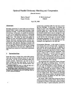
Early applications of decision-bound theory freely estimated a suboptimal decision criterion, b, from the data (i.e., b replaced bo in Equation 5; see Maddox, 2002, for a review). One weakness of this approach is that no mechanism was formalized to guide decision criterion placement. Maddox and Dodd (2001) offered a formal theory of decision criterion learning that uses decisionbound theory as the basic modeling framework, but supplements the model by postulating psychologically meaningful mechanisms that guide decision criterion placement. In other words, instead of simply estimating the decision criterion value directly from the data, Maddox and Dodd outlined formal processes that determine the decision criterion value. The theory proposes two mechanisms that determine decision criterion placement. Before we outline these two mechanisms, it is important to reiterate that the theory has its roots in signal detection theory, and thus makes use of parametric properties of stimulus distributions, likelihood ratios, likelihood ratiobased decision criteria, and related constructs. Even so, although these constructs help us to understand and characterize decision criterion learning behavior, we are not arguing that people possess explicit information about the stimulus distributions, likelihood ratios, or decision criteria. People gain information (likely implicitly3) about the categorization problem by experiencing stimuli and the reinforcing consequences of the decisions they make (i.e., their reinforcement history). There are likely many mathematical systems (or algorithms) that can capture the behavioral profile of decision criterion learning, and ours is only one of them. Even so, our approach provides insight into categorization behavior and leads to testable predictions. COBRA and COBRM Hypotheses COBRA. The COBRA hypothesis postulates that observers attempt to maximize expected reward (in consistency with instructions and monetary compensation contingencies), but they also place importance on accuracy maximization. Consider the univariate categorization problems depicted in Figure 1. Panel A displays a 3:1 base-rate (3:1B) condition, and panel B displays a 3:1 payoff (3:1P) condition. Expected reward is maximized in both cases by using the optimal reward-maximizing decision criterion, k ro 5 ln(b ro)/d ¢ 5 ln(3)/d ¢ (Equation 2). Thus, an observer who attempts to maximize expected reward should use the same decision criterion in both conditions. In the 3:1B condition, the decision criterion that maximizes reward also maximizes accuracy, so kao 5 k ro, but in the 3:1P condition the accuracy-maximizing decision criterion is different from the reward-maximizing decision criterion. Specifically, in the 3:1P condition, kao 5 ln(bao)/d ¢ 5 ln(1)/d ¢. (When base rates are equal,
MATCHING, MAXIMIZING, AND THE INDEPENDENCE ASSUMPTION
107
decision criterion, k ro 5 ln(b ro)/d ¢ 5 ln(3)/d ¢. In the 3:1B condition, the probability-matching decision criterion (k m ) is different from the reward-maximizing decision criterion (k ro), and so both goals cannot be achieved simultaneously. (Recall that reward and accuracy maximization can be achieved simultaneously in this condition; see Figure 1A.) Similarly, in the 3:1P condition, the probability-matching decision criterion is different from the reward-maximizing decision criterion. However, in this case the probability-matching and accuracy-maximizing decision criteria are identical (compare Figures 1B and 2B). Thus, COBRA and COBRM make identical predictions when only payoffs are manipulated, but make different predictions whenever base rates are manipulated. To instantiate COBRM within Maddox and Dodd’s (2001) hybrid model framework, we used the same weighting function outlined above but replaced ka with km. Specifically, we assume that k 5 wkm 1 (1 2 w) k r , where w (0 ² w ² 1) denotes the weight placed on probability matching.
Figure 1. Schematic illustration of the competition between reward and accuracy maximization (COBRA) hypothesis (see text for details).
it is always the case that the accuracy-maximizing decision criterion bao 5 1.) Thus, reward and accuracy can be simultaneously maximized in base-rate conditions but not in payoff conditions. An observer who places importance on both goals will use a decision criterion intermediate between the accuracy- and reward-maximizing decision criteria in the payoff condition. Maddox and Dodd (2001) instantiated COBRA by assuming a simple weighting function, k 5 wka 1 (1 2 w) kr , where w (0 ² w ² 1) denotes the weight placed on expected accuracy maximization yielding a single decision criterion intermediate between the accuracy- and reward-maximizing criteria.4 For example, in Figure 1B, k1 denotes a case in which w 5 .5. COBRM. The COBRM hypothesis postulates that observers attempt to maximize expected reward but also place importance on probability matching. The COBRM predictions for the 3:1B and 3:1P conditions are depicted in Figures 2A and 2B, respectively. Expected reward is maximized by the use of the optimal reward-maximizing
Figure 2. Schematic illustration of the competition between reward maximization and probability matching (COBRM ) hypothesis (see text for details).
108
MADDOX AND BOHIL
Flat-Maxima and Independence Predictions for Simultaneous Base-Rate/Payoff Conditions The flat-maxima hypothesis determines the rewardmaximizing decision criterion, k r (Busemeyer & Myung, 1992; von Winterfeldt & Edwards, 1982). Suppose that the observer adjusts the decision criterion on the basis of the change in the rate of reward, with larger changes in rate being associated with faster, more nearly optimal decision criterion learning (see, e.g., Busemeyer & Myung, 1992; Dusoir, 1980; Erev, 1998; Erev, Gopher, Itkin, & Greenshpan, 1995; Kubovy & Healy, 1977; Roth & Erev, 1995; Thomas, 1975; Thomas & Legge, 1970). To formalize this hypothesis, we construct the objective reward function, which plots objective expected reward on the y-axis and the decision criterion value on the x-axis. To generate an objective reward function, one chooses a value for the decision criterion and computes the expected reward for that criterion. This process is repeated over a range of criterion values. The expected reward is then plotted as a function of the deviation between a hypothetical observer’s decision criterion ln(b) and the optimal decision criterion ln(bo) standardized by category d ¢, where d ¢ is defined as the standardized distance between the category means and equals 2.2 in the present study. This is referred to as k 2 ko 5 ln( b)/d ¢ 2 ln(bo)/d ¢. In Figure 3A, the objective reward functions are plotted for separate 3:1B and 2:1P base-rate/payoff conditions and for a 3:1B/2:1P corresponding simultaneous base-rate/payoff condition. The derivative of the objective reward function at a specific k 2 ko value determines the change in the rate of expected reward for that k 2 ko value; the larger the change in the rate, the steeper the objective reward function will be at that point. The same fixed derivative for each of the three functions is denoted by the three tangent lines in Figure 3A. Figure 3B displays the associated steepness functions. The tangent lines in Figure 3A correspond to the k 2 k o values associated with the same steepness value for the 3:1B, 2:1P, and 3:1B/2:1P conditions. The horizontal line in Figure 3B denotes the associated steepness value, and the vertical lines denote the associated k 2 ko values for each condition. For this fixed steepness value, k 2 ko equals 2.40 in the 3:1B condition, 2.37 in the 2:1P condition, and 2.45 in the 3:1B/2:1P condition. Of interest is a comparison of the flat-maxima hypothesis prediction for the 3:1B/2:1P condition with the associated prediction from the independence assumption of the optimal classifier. In deriving the independence assumption prediction, we assumed that the flat-maxima hypothesis determined the decision criterion for the 3:1B and 2:1P conditions as outlined above, yielding k 2 ko values of 2.40 in the 3:1B condition and 2.37 in the 2:1P condition. We then combined them using the independence assumption of Equation 3 to yield the 3:1B/2:1P k 2 ko value of 2.77 predicted from the independence assumption. This k 2 ko value is denoted by the asterisk on the x-axis in Figures 3A and 3B. Notice that the k 2 ko value for the 3:1B/2:1P condition predicted directly from
Figure 3. (A) Objective reward functions for 3:1B, 2:1P, and 3:1B/2:1P conditions. The tangent lines, one for each condition, have the same slope, and thus reflect the same derivative or steepness. (B) Steepness of the objective rewa rd functions from panel A along with the three “equal steepness” points as denoted by the horizontal line. The decision criterion predicted from the independence assumption is denoted by the asterisk on the x-axis. Notice that the flat-maxima hypothesis predicts more nearly optimal decision criterion learning in the 3:1B/2:1P condition than the independence assumption does.
the flat-maxima hypothesis(2.45) is closer to optimal than that predicted from the independence assumption (2.77). To determine whether the flat-maxima hypothesis always predicts more nearly optimal decision criterion placement in the 3:1B/2:1P condition than the independence assumption does, we repeated this process across a large number of steepness values (specifically, steepness values ranging from the optimal value of 0 to the steepness associated with b 5 1 or, equivalently, ln( b) 5 0). The results are plotted (in the absolute value of the natural log–natural log space) in Figure 4C. In this and the other panels of Figure 4, the solid line denotes the relationship between the flat-maxima and independence predictions, and the broken line is included for comparative purposes and denotes situations in which the two hy-
MATCHING, MAXIMIZING, AND THE INDEPENDENCE ASSUMPTION
109
Figure 4. Absolute value of the decision criterion [ln(b )] predicted from the flat-maxima hypothesis plotted against the absolute value of the decision criterion [ln(b )] predicted from the independence assumption of the optimal classifier for the simultaneous base-rate/payoff conditions. See text for details of the procedure used to generate predicted decision criterion values.
potheses make identical predictions. The x-axis displays the criterion values derived from the independence assumption, and the y-axis displays the criterion values predicted from the flat-maxima hypothesis. For the 3:1B/2:1P condition, it is always the case that the solid line lies above the broken line, indicating that the flatmaxima hypothesis always predicts more nearly optimal decision criterion placement than the independence assumption. [Of course, the predictions converge at ln(bo).] The same approach was taken for the 2:1B/3:1P condition and yielded identical results. In addition, because of symmetry in the objective reward functions, the same result holds for the 1:2B/1:3P and 1:3B/1:2P conditions (it is for this reason that the results are plotted as absolute values). We repeated the same process for the remaining corresponding simultaneous base-rate/payoff conditions. The results for the 2:1B/2:1P and 1:2B/1:2P conditions are displayed in Figure 4A. The results for the 3:1B/3:1P and 1:3B/1:3P conditions are displayed in
Figure 4B. Across all 8 corresponding simultaneous base-rate/payoff conditions, the flat-maxima hypothesis predicts more nearly optimal decision criterion learning than does the independence assumption of the optimal classifier. The same approach was applied to the 1:2B/3:1P, 3:1B/1:2P, 1:3B/2:1P, and 2:1B/1:3P conflicting simultaneous base-rate/payoff conditions. The results were identical across all four conditions and are displayed in Figure 4D. Notice that, in contrast with the finding for the corresponding simultaneous base-rate/payoff conditions, for these conflicting base-rate/payoff conditions the solid line falls below the broken line, signifying that the flat-maxima hypothesis predicts the use of a decision criterion that is farther from optimal than that predicted by the independence assumption. Figure 4 excludes predictions from the remaining four conflicting simultaneous base-rate/payoff conditions, specifically, the 2:1B/1:2P, 1:2B/2:1P, 3:1B/1:3P, and 1:3B/3:1P conditions. Be-
110
MADDOX AND BOHIL
cause our approach assumes that the steepness of the objective reward function determines the decision criterion used in the separate base-rate/payoff conditions, and because the objective reward functions are symmetric across conflicting conditions that “cancel out” (e.g., 2:1B and 1:2P), the independence assumption always predicts the use of the optimal decision criterion. Depending on the steepness value, the flat-maxima hypothesis can predict decision criteria on either side of the optimal value. The Hybrid Model Framework COBRA version. Maddox and Dodd’s (2001) hybrid model of decision criterion learning assumes that the decision criterion used by the observer to maximize expected reward (kr ) is determined by the steepness of the objective reward function. A single steepness parameter is estimated from the data that determines a distinct decision criterion in every condition that has a unique objective reward function. The COBRA hypothesis is instantiated in the hybrid model by estimating the accuracy weight, w, from the data. To facilitate the development of each model, consider the following equation, which determines the decision criterion used by the observer on condition i trials (ki): ki 5 wkai 1 (1 2 w)kri .
(6)
Importantly, when base rates are manipulated, the observer’s estimate of the reward-maximizing decision criterion, derived from the flat-maxima hypothesis, is also the best estimate of the accuracy-maximizing decision criterion, resulting not in competition but simply in the use of the observer’s estimate of the reward-maximizing decision criterion. When payoffs are manipulated, on the other hand, the reward- and accuracy-maximizing decision criteria differ from one another. By pretraining each observer on the category structures in a baseline condition (described shortly in the Method section), we essentially pretrain the accuracy-maximizingdecision criterion. This criterion is then entered into the weighting function along with the observer’s estimate of the reward-maximizing decision criterion to determine the criterion used on each trial in the experimental conditions. COBRM version. The COBRM version of the hybrid model incorporates the flat-maxima hypothesis exactly
as described above. The COBRM hypothesis is instantiated in the hybrid model by estimating the probability matching weight, w, from the data. Taken together, the decision criterion used by the observer on condition i trials (ki ) is ki 5 wk mi 1 (1 2 w)k ri .
(7)
Because k m does not equal k r in any of the base-rate/payoff conditions used in the present study (except the baseline condition), this model predicts a competition between reward maximization and probability matching in all conditions. All of the models developed in this article are based on the decision-bound model in Equation 5 and include one “noise” parameter for each block of trials that represent the sum of perceptual and criterial noise (Ashby, 1992a; Maddox & Ashby, 1993). To ensure that the observers had adequate knowledge of the category structures [lo(x pi )], we pretrained each observer on the category structures in the baseline condition (described in the Method section). The nested structure of the models is presented in Figure 5, with each arrow pointing to a more general model and models at the same level having the same number of free parameters. The numbers of free parameters (in addition to the noise parameters described above) are presented in parentheses. (The details of the model-fitting procedure are outlined in the Results section.) The Hybrid(COBRA) and Hybrid(COBRM) models instantiate both the flat-maxima and the COBRA and COBRM hypotheses, respectively. To instantiate the flatmaxima hypothesis, a single steepness parameter is estimated from the data. This single steepness parameter determines 13 distinct k r values: (1) 2:1B and 2:1P, (2) 1:2B and 1:2P, (3) 3:1B and 3:1P, (4) 1:3B and 1:3P, (5) 2:1B/2:1P, (6) 1:2B/1:2P, (7) 3:1B/3:1P, (8) 1:3B/1:3P, (9) 2:1B/3:1P and 3:1B/2:1P, (10) 1:2B/1:3P and 1:3B/1:2P, (11) 1:2B/3:1P and 3:1B/1:2P, (12) 2:1B/1:3P and 1:3B/2:1P, and (13) 1:1B/1:1P, 1:2B/2:1P, 2:1B/1:2P, 1:3B/3:1P, and 3:1B/1:3P. To instantiate COBRA, the w parameter from Equation 6 was freely estimated, and to instantiate COBRM the w parameter from Equation 7 was freely estimated. More general versions of the Hybrid(COBRA) and Hybrid(COBRM) models were applied to the data. The Hybrid(COBRA; wP; w Corresponding;
Figure 5. Nested relationship among the models applied simultaneously to the data from all experimental conditions. The numbers in parentheses denote the numbers of free parameters in addition to the noise parameter. Each arrow points to a more general model (see text for details).
MATCHING, MAXIMIZING, AND THE INDEPENDENCE ASSUMPTION wConflicting) and Hybrid(COBRM; wP ; wCorresponding; wConflicting ) models estimated three accuracy weights. One was applied to the four separate payoff conditions (i.e., 2:1P, 1:2P, 3:1P, and 1:3P), a second was applied to the eight corresponding simultaneous base-rate/payoff conditions (i.e., 2:1B/2:1P, 1:2B/1:2P, 3:1B/3:1P, 1:3B/1:3P, 2:1B/3:1P, 1:2B/1:3P, 3:1B/2:1P, and 1:3B/1:2P), and a third was applied to the eight conflicting simultaneous base-rate/payoff conditions (i.e., 1:2B/3:1P, 2:1B/1:3P, 3:1B/1:2P, 1:3B/2:1P, 1:2B/2:1P, 2:1B/1:2P, 1:3B/3:1P, and 3:1B/1:3P). Variants of the Hybrid(COBRA) and Hybrid(COBRM) models that instantiated the independence assumption were also developed. The Hybrid (COBRA)-independence model applied the Hybrid (COBRA) model framework to determine the decision criteria in the separate base-rate and payoff conditions and then combined these independently to derive the decision criteria in the simultaneous base-rate/payoff conditions. The Hybrid(COBRM)-independence model applied the Hybrid(COBRM) model framework in the same manner. Simpler models, such as those that instantiate only the flat-maxima, the COBRA, or the COBRM hypothesis, were also applied to the data. They rarely provided the best account of the data, and since the focus of this work was on the hybrid model and the COBRA/ COBRM distinction, these models are not discussed. EXPERIMENT In this article, we report the results of a categorization experiment in which we examined decision criterion learning in 25 base-rate/payoff conditions constructed from the factorial combinationof five base-rate ratios (1:3, 1:2, 1:1, 2:1, and 3:1) with five payoff ratios (1:3, 1:2, 1:1, 2:1, and 3:1), yielding a large number of separate, corresponding simultaneous, and conflicting simultaneous base-rate/payoff conditions. We used these data to provide a critical comparison of the COBRA and COBRM hypotheses, and as an extensive and powerful test of the flatmaxima hypothesis and the independenceassumption predictions outlined in Figure 4. To achieve these goals, we had each observer complete three blocks of trials in all 25 base-rate/payoff conditions, and then we simultaneously applied each of the models presented in Figure 5 to the data from all 25 experimental conditions and all three blocks, separately for each observer. All analyses were performed at the individual observer level because of concerns with modeling aggregate data (see, e.g., Ashby, Maddox, & Lee, 1994; Estes, 1956; Maddox, 1999; Maddox & Ashby, 1998; J. D. Smith & Minda, 1998). Method Observers. Eight observers were solicited from the University of Texas community. All observers claimed to have 20/20 vision or vision corrected to 20/20. Each observer completed the baseline condition on the first day, followed by eight sessions of approximately 60 min. In each of the eight sessions, the observers completed three base-rate/ payoff conditions. The order of the latter 24 conditions was determined from a Latin square. The observers were paid on the basis of their performance on the task.
111
Stimuli and stimulus generation . The stimulus was a filled white rectangular bar that varied in height from trial to trial (40 pixels wide) set flush on a stationary base (60 pixels wide). There were two categories of bar heights, A and B, each defined by a specific univariate normal distribution (Ashby & Gott, 1988). The separation between the Category A and B means was 45 pixels, with an SD of 21 pixels for both categories, yielding a category d ¢ of 2.2. Five sets of 60 stimuli were generated prior to the experiment. One set contained 30 A and 30 B stimuli and was used in all cases for which the base rates were equal—that is, in the 2:1P, 1:2P, 3:1P, and 1:3P baseline conditions (to be described shortly). The second contained 40 A and 20 B stimuli and was used in all cases with a 2:1 base rate—that is, in the 2:1B, 2:1B/2:1P, 2:1B/1:2P, 2:1B/3:1P, and 2:1B/1:3P conditions. The third contained 45 A and 15 B stimuli and was used in all cases with a 3:1 base rate—that is, in the 3:1B, 3:1B/3:1P, 3:1B/1:3P, 3:1B/2:1P, and 3:1B/1:2P conditions. The fourth contained 20 A and 40 B stimuli and was used in the 1:2B, 1:2B/1:2P, 1:2B/1:3P, 1:2B/2:1P, and 1:2B/3:1P conditions. The fifth contained 15 A and 45 B stimuli and was used in the 1:3B, 1:3B/1:2P, 1:3B/1:3P, 1:3B/2:1P, and 1:3B/3:1P conditions. Each stimulus set was generated by taking numerous random samples (of size 60) from the population and selecting the sample whose objective reward function was most similar (on the basis of visual inspection) to that derived from the population. Two measures were taken to discourage information transfer across conditions. First, and most importantly, prior to the start of each of the 25 base-rate/ payoff conditions, the observer completed a minimum of 60 baseline trials in which the base rates were equal and the payoffs were equal. If the observer reached an accuracy-based performance criterion (no more than 2% below optimal), then two decision-bound models were fit to the 60 trials of data (see Maddox & Bohil, 1998, for details). The optimal decision criterion model assumed that the observer used the optimal decision criterion (i.e., b 5 1) in the presence of perceptual and criterial noise, whereas the free decision criterion model estimated the observer’s decision criterion from the data. Because the optimal decision criterion model is a special case of the free decision criterion model, likelihood ratio tests were used to determine whether the extra flexibility of the free decision criterion model provided a significant improvement in fit. If the free decision criterion model did not provide a significant improvement in fit over the optimal decision criterion model, then the observer was allowed to begin the experimental condition. If the free decision criterion model did provide a significant improvement in fit, then the observer completed 10 additional trials, and the same accuracy-based and model-based criteria were applied to the most recent 60 trials (i.e., Trials 11–70). This procedure continued until the observer reached the appropriate criterion. The inclusion of these baseline trials and this fairly conservative accuracy-base d and model-based performance criteria ensured that each observer had accurate knowledge of the category structures before exposure to the base-rate or payoff manipulation and minimized the possibility of within-observer carry-over effects from one experimental condition to the next. As an additional safeguard, different category labels were used (e.g., “burlosis” and “namitis” in one condition, and “coralgia” and “terragitis” in another condition) across the 25 experimental conditions. Each experimental condition consisted of three 60-trial blocks during which corrective feedback was provided on each trial (see details below). The same 60 stimuli were presented (in random order) once in each block. The base rates, payoffs, point totals, accuracy rates, b, and ln( b) values for the optimal classifier are displayed in Table 2, separately for each condition. Procedure. The observers were told that perfect performance was impossible, but an optimal level of performance was specified as a goal (in the form of desired point totals) in each condition. The observers were told that they were participating in several hypothetical medical diagnosis tasks and that the length of the bar represented the results of a particular medical test. The test was designed to distinguish between two diseases, such as “burlosis” and “namitis” (hereafter referred to simply as members of Category A
112
MADDOX AND BOHIL Table 2 Category Base Rates, Payoffs, Optimal Points (per 60-Trial Block), Accuracy, b, and ln(b ) Values for the 25 Base-Rate/Payoff Conditions Base Rates Condition
p(A)
p(B)
Baseline
.50
.50
2:1B 1:2B 2:1P 1:2P 3:1B 1:3B 3:1P 1:3P
.67 .33 .50 .50 .75 .25 .50 .50
.33 .67 .50 .50 .25 .75 .50 .50
2:1B/2:1P 1:2B/1:2P 3:1B/3:1P 1:3B/1:3P 2:1B/3:1P 1:2B/1:3P 3:1B/2:1P 1:3B/1:2P
.67 .33 .75 .25 .67 .33 .75 .25
2:1B/1:2P 1:2B/2:1P 3:1B/1:3P 1:3B/3:1P 1:2B/3:1P 2:1B/1:3P 3:1B/1:2P 1:3B/2:1P
.67 .33 .75 .25 .33 .67 .75 .25
Payoffs VaA
VbB
Points
6 6 308 Separate Base-Rate/Payoff Conditions 6 6 314 6 6 314 8 4 314 4 8 314 6 6 319 6 6 319 9 3 319 3 9 319
Accuracy
bo
ln(bo)
85.5
1
87.1 87.1 84.7 84.7 88.7 88.7 82.9 82.9
2 .5 2 .5 3 .33 3 .33
0.69 20.69 0.69 20.69 1.10 21.10 1.10 21.10
Corresponding Simultaneous Base-Rate/Payoff Conditions .33 8 4 360 86.1 .67 4 8 360 86.1 .25 9 3 421 86.7 .75 3 9 421 86.7 .33 9 3 386 84.7 .67 3 9 386 84.7 .25 8 4 386 87.8 .75 4 8 386 87.8
4 .25 9 .11 6 .17 6 .17
1.39 21.39 2.20 22.20 1.79 21.79 1.79 21.79
Conflicting Simultaneous Base-Rate/Payoff Conditions .33 4 8 275 85.5 .67 8 4 275 85.5 .25 3 9 232 85.5 .75 9 3 232 85.5 .67 9 3 259 84.1 .33 3 9 259 84.1 .25 4 8 259 87.6 .75 8 4 259 87.6
1 1 1 1 1.5 .67 1.5 .67
0 0 0 0 0.41 20.41 0.41 20.41
and of Category B, respectively). The observers were informed that they would receive the medical test result for a new patient on each trial, and that the goal was to maximize points in each condition. They were informed that these point totals would be converted into monetary values that they would receive at the end of the experiment. The observers were instructed to maximize points and not to worry about speed of responding. They were informed of the baserate and /or payoff ratio at the start of each condition. A typical trial proceeded as follows. A stimulus was presented on the screen and remained until a response was made. The observer’s task was to classify the presented stimulus as a member of Category A or Category B by pressing the appropriate button. The observer’s response was followed by 750 msec of feedback. Five lines of feedback were presented. The first (top) line indicated the correct disease label on that trial. The second line indicated the points earned on that trial. The third line indicated the value of a correct response (i.e., the potential points) for that trial (independent of the observer’s response). The fourth line indicated the total points earned to that point in the experiment, and the fifth (bottom) line indicated the maximum total points (i.e., potential total points) that could have been earned to that point in the experiment (independent of the observer’s performance). The feedback was followed by a 125-msec intertrial interval during which the screen was blank. The observers were given a break after each block of trials. At each break, the observer’s accumulated point total was displayed.
Results and Theoretical Analysis Each of the models presented in Figure 5 was applied simultaneously to the data from all 25 experimental condi-
0
tions and three blocks separately by observer. Each block consisted of 60 experimental trials, and the observer was required to respond “A” or “B” for each stimulus. Thus, across the three blocks of trials each model was fit to a total of 9,000 estimated response probabilities[60 trials 3 2 response types (“A” or “B”) 3 25 conditions 3 3 blocks]. Since the predicted probability of responding “B,” p(“B”), equals 12p(“A”), there were 4,500 degrees of freedom. Maximum likelihoodprocedures (Ashby, 1992b; Wickens, 1982) were used to estimate the model parameters with the goal of minimizing 2lnL. The most parsimonious model was defined as the model with the fewest free parameters for which a more general model did not provide a statistically significant improvement in fit on the basis of likelihood ratio (G 2) tests with a 5 .05 (for a discussion of the complexitiesof model comparison, see Myung, 2000; Pitt, Myung, & Zhang, 2002). Under the null hypothesis of equally good fit, G 2 is distributed as c 2. Table 3 displays the maximum likelihoodfit value along with the percent of responses accounted for (averaged across observers) for all models presented in Figure 5 (the smaller the value, the better the fit). Although the most parsimonious model was determined from the simultaneous fit across blocks (the Total column in Table 3), some interesting results emerged from an examination of the goodness of fit of each block, and so these values are also included.
MATCHING, MAXIMIZING, AND THE INDEPENDENCE ASSUMPTION
113
Table 3 Maximum Likelihood Fit Value (2lnL) and Percent of Responses Accounted for (Averaged Across Observers) for Several Models Applied Simultaneously to the Data From All 25 Experimental Conditions, by Block Block Model
1
2
3
Maximum Likelihood Fit Value (2lnL) Hybrid(COBRA) 395.06 364.90 388.98 Hybrid(COBRM) 385.59 364.60 395.62 Hybrid(COBRA; wP ; wCorresponding ; wConflicting) 388.64 362.72 377.32 Hybrid(COBRM; wP; wCorresponding ; w Conflicting) 382.72 361.62 391.89 Hybrid(COBRA)-independence 395.97 365.07 396.44 Hybrid(COBRM)-independence 385.05 366.00 400.44 Percent of Responses Accounted For Hybrid(COBRA) 90.38 90.37 Hybrid(COBRM) 90.49 90.33 Hybrid(COBRA; wP ; wCorresponding ; wConflicting) 90.76 91.44 Hybrid(COBRM; wP; wCorresponding ; w Conflicting) 90.54 90.50 Hybrid(COBRA)-independence 90.25 90.38 Hybrid(COBRM)-independence 90.48 90.27
Because the COBRA models form an efficient nesting and the COBRM models form a similar nesting, we decided to conduct the likelihood ratio tests separately for each pair of models and then compare the best fitting version of COBRA and COBRM from each set directly. We could have compared the full set of models to determine the best fitting model, but some models are not nested [e.g., Hybrid(COBRA) and COBRM], and so would require a mixture of likelihood ratio testing for nested models and some other approach, such as AIC, for nonnested models. Most parsimonious COBRA or COBRM model. To determine whether the Hybrid(COBRA; wP; wCorresponding; wConflicting) model provided a better account of the data than the Hybrid(COBRA) model, we conducted likelihood ratio tests. The G2 values ranged from 21.48 to 70.48, falling above the critical value of 12.59 (a 5 .05, with 6 degrees of freedom) for all 8 observers. Notice that the performance of the Hybrid(COBRA; wP; w Corresponding; w Conflicting) model was quite good, accounting for over 91% of the responses in the data. We took the same approach to determine whether the Hybrid(COBRM; wP; w Corresponding; w Conflicting) model provided a better account of the data than the Hybrid (COBRM) model. The G 2 values ranged from 5.50 to 38.65, falling above the critical value of 12.59 (a 5 .05, with 6 degrees of freedom) for 4 of the 8 observers. The fit of the Hybrid(COBRM; wP; wCorresponding; w Conflicting) model was quite good, accounting for over 90% of the responses in the data. COBRA versus COBRM versions. Because the Hybrid(COBRA; wP; w Corresponding; w Conflicting) model was superior for all 8 observers in the COBRA set of models and because the Hybrid(COBRM; w P; w Corresponding ; wConflicting) model was superior for 4 of the 8 observers in the COBRM set of models, we focus on these two models. A direct comparison of the fit values reveals that the
90.65 90.22 91.02 90.30 90.09 90.07
Total
Average
1,148.94 1,145.81 1,128.69 1,136.23 1,157.47 1,151.49 90.46 90.35 91.07 90.45 90.24 90.28
COBRM version provided a better account of the data for 5 of the 8 observers, and the COBRA version provided a better account of the data for the remaining 3 observers, suggesting no strong advantage for one version over the other. To gain a more detailed understanding of the predictive power of the COBRA and COBRM hypotheses, we decided to partition the maximum likelihood fit summed over blocks into a separate fit value for each block. Previous work by Ashby and colleagues (Ashby & Maddox, 1993; Maddox & Ashby, 1993) indicated that observers have a tendency to shift from responding more in line with probability matching to responding more in line with maximization as they gain experience with a task. On the basis of these results, our speculation was that the Hybrid(COBRM; wP ; wCorresponding; wConflicting) model might provide a superior account of the data early in learning, whereas the Hybrid(COBRA; wP; wCorresponding; wConflicting) model might provide a superior account of the data late in learning. Notice that this pattern held in the averaged fit values outlined in Table 3 with a better average fit for the Hybrid(COBRM; wP; wCorresponding; wConflicting) model during the first block of trials, a better average fit for the Hybrid(COBRA; w P; w Corresponding; w Conflicting) model during the third block of trials, and nearly identical average fits for both models during the second block of trials. To determine whether this pattern held at the level of the individual observer, we compared the fit values on a block-by-block basis. As we expected, the fit of the Hybrid(COBRM; wP; w Corresponding; wConflicting) model was superior to that of the Hybrid(COBRA; wP; wCorresponding; wConflicting) model for 6, 4, and 0 of 8 observers in Blocks 1 to 3, respectively. Thus, it appears that the observers entered the experiment with a bias toward a competition between reward maximization and probability matching, and, with experience, the bias shifted toward a competition between reward and accuracy maximization. To see
114
MADDOX AND BOHIL
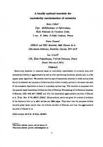
if this pattern replicates, we reanalyzed the data from Bohil and Maddox (2003) by comparing fits of the Hybrid(COBRM; wP; wCorresponding; wConflicting) and Hybrid (COBRA; wP; w Corresponding; wConflicting ) models. Bohil and Maddox had 15 observers complete 3 training blocks and one test block in 10 of the 25 base-rate/payoff conditions from the present study (see Table 1). For 8, 5, 10, and 10 of the 15 observers in Training Blocks 1–3 and the test block, respectively, the Hybrid(COBRA; wP; w Corresponding; wConflicting) model provided a superior account of the data, generally replicating the pattern observed in the present study. The steepness and weight parameters (w) from the Hybrid(COBRA; wP; w Corresponding; wConflicting) and Hybrid (COBRM; wP; wCorresponding; wConflicting) models are displayed for the three blocks of trials averaged across observers in Figure 6. Several results stand out. First, a one-way ANOVA on the steepness values revealed a nonsignificant effect of block [COBRA version: F(2,14) 5 1.97, p . .05; COBRM version: F(2,14) 5 1.66, p . .05] but a clear monotonic trend toward the optimal rewardmaximizing decision criterion over blocks from both models. Second, a two-way ANOVA on the accuracy and
probability matching weight (w) values revealed a significant condition 3 block interaction for both models [COBRA version: F(4,28) 5 4.78, p , .01; COBRM version: F(4,28) 5 8.16, p , .01]. This interaction was characterized by a weight applied to the separate payoff conditions that remained fairly constant across blocks, a weight applied to the corresponding simultaneous baserate/payoff conditions that generally declined across blocks, and a weight applied to the conflicting simultaneous base-rate/payoff conditions that generally increased across blocks. The main effects of condition and block were nonsignificant for both models. Interestingly, the pattern of weights over blocks was quite similar across the two models. Focusing on the final block and the Hybrid(COBRA; wP; wCorresponding; wConflicting) model, which fit best, notice that more weight was placed on accuracy maximization in the separate payoff conditions than in either type of simultaneous base-rate/payoff condition. A similar pattern was observed by Bohil and Maddox (2003). Tests of the flat-maxima and independence assum ption predictions. With no additional post hoc mechanisms, the COBRA and COBRM instantiations of
Figure 6. Steepness values from the (A) Hybrid(COBRA; w P; w Corresponding ; w Conflicting ) model and (B) Hybrid(COBRM; w P; w Correw Conflicting ) model for the three blocks averaged across observers, and accuracy weights (w) from the (C) Hybrid(COBRA; w P; w Corresponding ; wConflicting ) model and (D) Hybrid(COBRM; wP; w Corresponding ; w Conflicting ) model for the three blocks averaged across observers. Standard error bars are included.
sponding ;
MATCHING, MAXIMIZING, AND THE INDEPENDENCE ASSUMPTION the hybrid model captured performance across all 25 baserate/payoff conditions. The good fits of the hybrid model are promising, but a direct comparison of the hybrid model with a model that assumes an independent combination of base-rate and payoff information in the simultaneous base-rate/payoff conditions is in order. To achieve this goal, we developed two models: the Hybrid (COBRA)-independencemodel and the Hybrid (COBRM)independence model. These models both assume that the reward-maximizing decision criterion in the separate base-rate/payoff conditions are derived from the flatmaxima hypothesis, but that these are then combined independently (see Equation 3) to determine the decision criterion in the simultaneous base-rate/payoff conditions. These “independence” variants of the hybrid model have the same number of parameters as the Hybrid (COBRA) and Hybrid(COBRM) models, and so the fit values can be compared directly. These fit values and percent of variance accounted for (averaged across observers) are displayed in Table 3. For 7 of the 8 observers, the Hybrid(COBRA) model provided a better account of the data than did the Hybrid(COBRA)independence model, and for 6 of the 8 observers, the Hybrid(COBRM) model provided a better account of the data did than the Hybrid(COBRM)-independence model. Decision criterion estimates from signal detection theory. In this section, we examine decision criterion estimates derived from signal detection theory. Specifically, we computed the decision criterion for all 25 experimental conditions separately for each of the three blocks of trials and 8 observers from the hit rates and false alarm rates. We used these data to examine two issues. First, we were interested in determining whether performance in symmetric base-rate/payoff conditions (e.g., 3:1B/3:1P and 1:3B/1:3P) differed. To facilitate these analyses, we converted all conditions in which the optimal decision criterion, ko, was negativeto the associated positive ko condition (e.g., 1:3B/1:3P k values were converted to 2k to correspond with the 3:1B/3:1P condition).Second, we tested the flat-maxima hypothesis prediction that (1) decision criteria in corresponding simultaneous base-rate/payoff conditions should be closer to the optimal value than those predicted from the independence assumption and (2) decision criteria in conflicting simultaneous base-rate/payoff conditions will be farther from the optimal value than those predicted from the independence assumption. To determine whether performance differed across symmetric base-rate/payoff conditions, we conducted a series of two-tailed t tests. The k 2 k o values for each block averaged across observers and symmetric baserate/payoff conditions are displayed in Table 4, along with the t test results. In general, performance did not differ across symmetric base-rate/payoff conditions, with only 9 of the 36 tests revealing significant differences. In addition, 5 of these 9 were observed during the first block of trials, whereas only 1 was observed during the third block. In light of this fact, we focus the remaining analyses on the
115
Table 4 Deviation From Optimal Decision Criterion (k 2 k o ) Measure (Averaged Across Observers) by Condition and Block, and Significance Test Results Across Symmetric Base-Rate/Payoff Conditions Block Condition 2:1B 2:1P 3:1B 3:1P Average
1
2
3
Separate Base-Rate/Payoff Conditions 20.308** 20.291 20.221 20.264* 20.267* 20.239 20.327 20.171 20.228 20.427 20.452 20.412 20.331 20.295 20.275
Average 20.273 20.256 20.242 20.430 20.300
Corresponding Simultaneous Base-Rate/Payoff Conditions 2:1B/2:1P 20.434 20.289 20.177 20.300 3:1B/3:1P 20.695* 20.568 20.450 20.571 2:1B/3:1P 20.596 20.275 20.369 20.413 3:1B/2:1P 20.632* 20.415 20.320 20.456 Average 20.589 20.387 20.329 20.435 Conflicting Simultaneous Base-Rate/Payoff Conditions 1:2B/3:1P 20.216 20.266 20.262 20.248 3:1B/1:2P 20.205 20.086 0.021 20.090 2:1B/1:2P 0.101* 0.122* 0.006 20.077 3:1B/1:3P 0.075 20.031** 0.029** 20.024 Average 20.061 20.065 20.051 20.059 Overall Average 20.327 20.249 20.218 20.265 *p , .05. **p , .01.
data collapsed across symmetric base-rate/payoff conditions. To test the flat-maxima predictions regarding simultaneous base-rate/payoff conditions, we counted the number of times that the observed simultaneous baserate/payoff condition decision criterion was closer to optimal (for corresponding conditions) or was farther from optimal (for conflicting conditions) than the decision criterion predicted from an independent combination of the associated separate base-rate/payoff condition decision criteria. (Data from the 1:2B/2:1P, 2:1B/1:2P, 1:3B/3:1P, and 3:1B/1:3P conditions were excluded because the flatmaxima hypothesis can predict values that are either smaller or larger than those predicted from the optimal classifier; both are possible.) These data are summarized in Table 5 along with sign tests that were conducted assuming a null hypothesis probability of .50. Also included are the average difference between the observed and independence assumption predicted decision criteria and t test results on these data.5 Collapsed across blocks, the frequency counts and average differences are all in support of the flat-maxima hypothesis over the independence assumption, and the sign test and t test results in all but the 3:1B/2:1P (and 1:3B/1:2P) condition were either significant or marginally significant. Collapsed across simultaneous base-rate/payoff conditions, there was strong support for the flat-maxima hypothesis prediction over the independence assumption for all three blocks. These results mirror those obtained through the quantitative model-based analyses and provide strong support for the flat-maxima hypothesis over the independence assump-
116
MADDOX AND BOHIL Table 5 Frequency (No.) With Which the Observed Simultaneous Base-Rate/Payoff Condition Decision Criterion Was Closer to (for Corresponding) or Farther From (for Conflicting) the Optimal Value by Condition and Block, and Average Differences (M ) Block 1 Condition
No.
2 M
No.
3 M
No.
Total M
No.
M
2:1B/2:1P and 1:2B/1:2P 10/16 0.296 *12/16** 0.578† *12/16** 0.609** *34/48† 0.495** 3:1B/3:1P and 1:3B/1:3P *11/16* 0.126 9/16 0.118 9/16 0.409** *29/48* 0.218* 2:1B/3:1P and 1:2B/1:3P 10/16 0.298* 15/16† 1.009† *12/16** 0.571† *37/48† 0.626† 3:1B/2:1P and 1:3B/1:2P 6/16 20.088 7/16 0.047 *13/16** 0.316* 26/48 0.092 1:2B/3:1P and 2:1B/1:3P 9/16 20.267* 11/16* 20.359** 15/16† 20.586† *35/48† 20.404† 3:1B/1:2P and 1:3B/2:1P 16/16† 20.554** 16/16† 20.629** 16/16† 20.335* *48/48† 20.506** Total *57/96** 64/96† 72/96† *193/288† Note—There is no mean for the Total row because it would require averaging data from conditions for which a positive difference is predicted with conditions for which a negative difference is predicted. Sign test results assuming a null hypothesis probability 5 .50 and t test results assuming a null hypothesis mean of 0. *.05 , p , .10. **p , .05. †p , .01.
tion of the optimal classifier, which offers a theoretically motivated explanation of decision criterion placement in simultaneous base-rate/payoff conditions. GENERAL DISCUSSIO N Matching Versus Maximizing in Decision Criterion Learning All of our previous work with the hybrid model framework (see Maddox, 2002, for a review) assumed a COBRA. Even so, an important debate in the psychological literature is that between matching and maximizing strategies. This debate has not escaped the perceptual categorization literature, but has not been addressed in our decision-criterion learning work (e.g., Ashby & Maddox, 1993; Maddox & Ashby, 1993). In this study, we have developed and tested a COBRM hypothesis. An advantage of the present formulation and quantitative comparison is that the two approaches (COBRA and COBRM) are identical in their assumptions that the flatmaxima hypothesis determines the reward-maximizing decision criterion and that the observed decision criterion is a weighted function of reward and accuracy. The two formulations differ only in which aspect of accuracy is important (maximization or matching; compare Equations 6 and 7). Both approaches provide a good account of the data, but the COBRM approach generally dominates early in learning, whereas the COBRA approach dominates late in learning. In other words, behavior mimics probability matching early in learning and accuracy maximization late in learning. This finding is in accord with other results from the categorization literature. For example, Maddox and Ashby (1993) estimated a matching–maximizing parameter and found that the parameter value generally increased as the observer gained experience with the task, which is indicative of a shift from matching to maximizing. Although clearly more work is needed, to our knowledge this is one of the first attempts to compare rigorously matching and maximizing decision strategies within the same modeling framework (however, see Healy & Kubovy, 1981, for related work).
Flat-Maxima Versus Independence Assumption Predictions The flat-maxima hypothesis assumes that the decision criterion used by the observer to maximize expected reward is determined by the steepness of the objectivereward function. The flat-maxima hypothesis offers a priori predictions regarding decision criterion placement in separate and simultaneous base-rate/payoff conditions that were compared with predictions from the optimal classifier. Across a wide range of base-rate and payoff ratios totaling 25 separate conditions, the flat-maxima hypothesis provided a superior account of the data on the basis of quantitative fits of Maddox and Dodd’s (2001) hybrid model and decision criterion estimates from signal detection theory (Green & Swets, 1966; Macmillan & Creelman, 1991). The success of the flat-maxima hypothesis in accounting for these data, as well as numerous other situational variables such as category discriminability, base-rate/payoff ratio, and the magnitude of the payoff matrix entries, suggests that humans are (at least implicitly) sensitive to the steepness of the objective reward function. Summary In conclusion, the present study offers a rigorous model-based comparison of matching versus maximizing strategies that indicates that observers generally matched early in learning but quickly shifted toward a maximizing strategy with experience. This study also offers a comprehensive comparison of the flat-maxima hypothesis and independence assumption of the optimal classifier as applied to corresponding and conflicting simultaneous base-rate/payoff conditions. Strong support for the flat-maxima hypothesis over the independence assumption was found. REFERENCES Ashby, F. G. (1992a). Multidimensional models of categorization. In F. G. Ashby (Ed.), Multidimensional models of perception and cognition (pp. 449-484). Hillsdale, NJ: Erlbaum. Ashby, F. G. (1992b). Multivariate probability distributions. In F. G.
MATCHING, MAXIMIZING, AND THE INDEPENDENCE ASSUMPTION
Ashby (Ed.), Multidimensional models of perception and cognition (pp. 1-34). Hillsdale, NJ: Erlbaum. Ashby, F. G., Alfonso-Reese, L. A., Turken, A. U., & Waldron, E. M. (1998). A neuropsychological theory of multiple systems in category learning. Psychological Review, 105, 442-481. Ashby, F. G., & Ell, S. W. (2001). The neurobiological basis of category learning. Trends in Cognitive Sciences, 5, 204-210. Ashby, F. G., & Ell, S. W. (2002). Single versus multiple systems of learning and memory. In J. Wixted & H. Pashler (Eds.), Stevens’ Handbook of experimental psychology: Vol. 4. Methodology in experimental psychology (3rd ed., pp. 655-692). New York: Wiley. Ashby, F. G., & Gott, R. E. (1988). Decision rules in the perception and categorization of multidimensional stimuli. Journal of Experimental Psychology: Learning, Memory, & Cognition, 14, 33-53. Ashby, F. G., & Maddox, W. T. (1990). Integrating information from separable psychological dimensions. Journal of Experimental Psychology: Human Perception & Performance, 16, 598-612. Ashby, F. G., & Maddox, W. T. (1992). Complex decision rules in categorization: Contrasting novice and experienced performance. Journal of Experimental Psychology: Human Perception & Performance, 18, 50-71. Ashby, F. G., & Maddox, W. T. (1993). Relations between prototype, exemplar, and decision bound models of categorization. Journal of Mathematical Psychology, 37, 372-400. Ashby, F. G., Maddox, W. T., & Bohil, C. J. (2002). Observational versus feedback training in rule-based and information-integration category learning. Memory & Cognition, 30, 666-677. Ashby, F. G., Maddox, W. T., & Lee, W. W. (1994). On the dangers of averaging across subjects when using multidimensional scaling or the similarity-choice model. Psychological Science, 5, 144-150. Bohil, C. J., & Maddox, W. T. (2003). A test of the optimal classifier’s independence assumption in perceptual categorization. Perception & Psychophysics, 65, 478-493. Busemeyer, J. R., & Myung, I. J. (1992). An adaptive approach to human decision making: Learning theory, decision theory, and human performance. Journal of Experimental Psychology: General, 121, 177-194. Dusoir, A. E. (1980). Some evidence on additive learning models. Perception & Psychophysics, 27, 163-175. Erev, I. (1998). Signal detection by human observers: A cutoff reinforcement learning model of categorization decisions under uncertainty. Psychological Review, 105, 280-298. Erev, I., Gopher, D., Itkin, R., & Greenshpan, Y. (1995). Toward a generalization of signal detection theory to n-person games: The example of two-person safety problem. Journal of Mathematical Psychology, 39, 360-375. Erickson, M. A., & Kruschke, J. K. (1998). Rules and exemplars in category learning. Journal of Experimental Psychology: General, 127, 107-140. Estes, W. K. (1956). The problem of inference from curves based on group data. Psychological Bulletin, 53, 134-140. Estes, W. K. (1976). The cognitive side of probability learning. Psychological Review, 83, 37-64. Filoteo, J. V., Maddox, W. T., & Davis, J. D. (2001a). A possible role of the striatum in linear and nonlinear categorization rule learning: Evidence from patients with Huntington’s disease. Behavioral Neuroscience, 115, 786-798. Filoteo, J. V., Maddox, W. T., & Davis, J. D. (2001b). Quantitative modeling of category learning in amnesic patients. Journal of the International Neuropsychological Society, 7, 1-19. Galanter, E., & Holman, G. (1967). Some invariances of the isosensitivity function and their implications for the utility function of money. Journal of Experimental Psychology, 73, 333-339. Green, D. M., & Swets, J. A. (1966). Signal detection theory and psychophysics. New York: Wiley. Healy, A. F., & Kubovy, M. (1981). Probability matching and the formation of conservative decision rules in a numerical analog of signal detection. Journal of Experimental Psychology: Human Learning & Memory, 7, 344-354. Herrnstein, R. J. (1961). Relative and absolute strength of response as a function of frequency of reinforcement. Journal of the Experimental Analysis of Behavior, 4, 267-272.
117
Herrnstein, R. J. (1970). On the law of effect. Journal of the Experimental Analysis of Behavior, 13, 243-266. Herrnstein, R. J., & Heyman, G. M. (1979). Is matching compatible with reinforcement maximization on concurrent variable interval, variable ratio? Journal of the Experimental Analysis of Behavior, 31, 209-223. Kahneman, D., & Tversky, A. (1979). Prospect theory: An analysis of decision under risk. Econometrica, 47, 263-291. Knowlton, B. J., Mangels, J. A., & Squire, L. R. (1996). A neostriatal habit-learning system in humans. Science, 273, 1399-1402. Kornbrot, D., Donnelly, M., & Galanter, E. (1981). Estimates of utility function parameters from signal detection experiments. Journal of Experimental Psychology: Human Perception & Performance, 7, 441-458. Kubovy, M., & Healy, A. F. (1977). The decision rule in probabilistic categorization: What it is and how it is learned. Journal of Experimental Psychology: General, 106, 427-466. Macmillan, N. A., & Creelman, C. D. (1991). Detection theory: A user’s guide. New York: Cambridge University Press. Maddox, W. T. (1999). On the danger of averaging across observers when comparing decision bound models and generalized context models of categorization. Perception & Psychophysics, 61, 354-374. Maddox, W. T. (2002). Toward a unified theory of decision criterion learning in perceptual categorization. Journal of the Experimental Analysis of Behavior, 28, 1003-1018. Maddox, W. T., & Ashby, F. G. (1993). Comparing decision bound and exemplar models of categorization. Perception & Psychophysics, 53, 49-70. Maddox, W. T., & Ashby, F. G. (1998). Selective attention and the formation of linear decision boundaries: Comment on McKinley and Nosofsky (1996). Journal of Experimental Psychology: Human Perception & Performance, 24, 301-321. Maddox, W. T., & Bohil, C. J. (1998). Base-rate and payoff effects in multidimensional perceptual categorization. Journal of Experimental Psychology: Learning, Memory, & Cognition, 24, 1459-1482. Maddox, W. T., & Dodd, J. L. (2001). On the relation between baserate and cost-benefit learning in simulated medical diagnosis. Journal of Experimental Psychology: Learning, Memory, & Cognition, 27, 1367-1384. Maddox, W. T., & Estes, W. K. (1996, August). A dual process model of category learning. Paper presented at the 31st annual meeting of the Society for Mathematical Psychology, University of North Carolina, Chapel Hill. Maddox, W. T., & Filoteo, J. V. (2001). Striatal contribution to category learning: Quantitative modeling of simple linear and complex nonlinear rule learning in patients with Parkinson’s disease. Journal of the International Neuropsychological Society, 7, 710-727. Myung, I. J. (2000). The importance of complexity in model selection. Journal of Mathematical Psychology, 44, 190-204. Pickering, A. D. (1997). New approaches to study of amnesic patients: What can a neurofunctional philosophy and neural network methods offer? Memory, 5, 255-300. Pitt, M. A., Myung, I. J., & Zhang, S. (2002). Toward a method of selecting among computational models of cognition. Psychological Review, 109, 472-491. Roth, A. E., & Erev, I. (1995). Learning in extensive form games: Experimental data and simple dynamic models in the intermediate term. Games & Economic Behavior, 3, 3-24. Smith, E. E., Patalano, A. L., & Jonides, J. (1998). Alternative strategies of categorization. Cognition, 65, 167-196. Smith, J. D., & Minda, J. P. (1998). Prototypes in the mist: The early epochs of category learning. Journal of Experimental Psychology: Learning, Memory, & Cognition, 24, 1411-1436. Stevenson, M. K., Busemeyer, J. R., & Naylor, J. C. (1991). Judgment and decision-making theory. In M. D. Dunnette & L. M. Hough (Eds.), Handbook of industrial and organizationalpsychology (2nd ed., Vol. 1, pp. 283-374). Palo Alto, CA: Consulting Psychologist Press. Thomas, E. A. C. (1975). Criterion adjustment and probability matching. Perception & Psychophysics, 18, 158-162. Thomas, E. A. C., & Legge, D. (1970). Probability matching as a basis for detection and recognition decisions. Psychological Review, 77, 65-72.
118
MADDOX AND BOHIL
Tversky, A., & Kahneman, D. (1974). Judgment under uncertainty: Heuristics and biases. Science, 185, 1124-1131. Tversky, A., & Kahneman, D. (1980). Causal schemas in judgments under uncertainty. In M. Fishbein (Ed.), Progress in social psychology (pp. 72-94). Hillsdale, NJ: Erlbaum. Tversky, A., & Kahneman, D. (1992). Prospect theory: An analysis of decision under risk. Econometrica, 47, 276-287. von Winterfeldt, D., & Edwards, W. (1982). Costs and payoffs in perceptual research. Psychological Bulletin, 91, 609-622. Wickens, T. D. (1982). Models for behavior: Stochastic processes in psychology. San Francisco: Freeman. Williams, B. A. (1988). Reinforcement, choice, and response strength. In R. C. Atkinson, R. J. Herrnstein, G. Lindzey, & R. D. Luce (Eds.), Stevens’ Handbook of experimental psychology: Vol. 1. Perception and motivation (pp. 167-244). New York: Wiley. Yates, J. F. (1990). Judgment and decision-making. Englewood Cliffs, NJ: Prentice-Hall. NOTES 1. We are indebted to Ido Erev (personal communication, September, 2002) for suggesting the COBRM hypothesis. 2. The optimal decision criterion is constructed from the “objective” or “true” payoff information. Much work suggests that people do not use the objective values, but, rather, base their decisions on subjective values that are directly related to the objective values (see, e.g., Kahneman & Tversky, 1979; Stevenson et al., 1991; Tversky & Kahneman, 1974, 1980, 1992; Yates, 1990). Within the framework of decision theory, each of our ViJ terms should be converted into a subjective utility
denoted u(ViJ), where u describes the functional relationship between the subjective and objective values. In the case of points converted to money, it is reasonable to assume that increasing value is ordinally related to increasing utility. Several studies suggest that a power function with an exponent near .5 describes this relationship (Galanter & Holman, 1967; Kornbrot, Donnelly, & Galanter, 1981). All of the predictions outlined in this paper hold under this assumption. 3. The distinction between implicit and explicit memory and the importance of each system in category learning has received much attention in the past few years. The current thinking is that there are at least two category learning systems, one of which relies predominantly on explicit memory processes and the other predominantly on implicit memory processes (Ashby & Ell, 2001, 2002; Ashby, Maddox, & Bohil, 2002; Erickson & Kruschke, 1998; Pickering, 1997; E. E. Smith, Patalano, & Jonides, 1998). The neurobiological basis of these systems is an area of active research (Filoteo, Maddox, & Davis, 2001a, 2001b; Knowlton, Mangels, & Squire, 1996; Maddox & Filoteo, 2001; see Ashby & Ell, 2001, for a review). 4. Other methods for instantiating this competition are available (for related proposals, see Ashby, Alfonso-Reese, Turken, & Waldron, 1998; Maddox & Estes, 1996). The present approach is taken because it is easy to instantiate and has met with reasonable success (Maddox & Dodd, 2001). 5. Each observer provided two data points for each cell in Table 5 because we collapsed across symmetric base-rate/payoff conditions. (Manuscript received December 11, 2002; revision accepted for publication May 27, 2003.)