May 4, 2011 ... The last roll of the game in backgammon (splitting the stakes at Monte. Carlo). 4.
..... sit at a counter of 16 seats, the n runs of free and occupied seats determine a
partition k = 16 = k1 + ··· + kn. .... log x dx = (n + 1) log(n + 1) − n.
Probability Theory Course Notes — Harvard University — 2011
C. McMullen May 4, 2011
Contents I II III IV V VI VII VIII IX X XI XIV I II
The Sample Space . . . . . . . . . . . . . . . . . Elements of Combinatorial Analysis . . . . . . . Random Walks . . . . . . . . . . . . . . . . . . . Combinations of Events . . . . . . . . . . . . . . Conditional Probability . . . . . . . . . . . . . . The Binomial and Poisson Distributions . . . . . Normal Approximation . . . . . . . . . . . . . . . Unlimited Sequences of Bernoulli Trials . . . . . Random Variables and Expectation . . . . . . . . Law of Large Numbers . . . . . . . . . . . . . . . Integral–Valued Variables. Generating Functions Random Walk and Ruin Problems . . . . . . . . The Exponential and the Uniform Density . . . . Special Densities. Randomization . . . . . . . . .
. . . . . . . . . . . . . .
. . . . . . . . . . . . . .
. . . . . . . . . . . . . .
. . . . . . . . . . . . . .
. . . . . . . . . . . . . .
. . . . . . . . . . . . . .
. . . . . . . . . . . . . .
2 5 15 24 29 37 44 55 60 68 70 70 75 94
These course notes accompany Feller, An Introduction to Probability Theory and Its Applications, Wiley, 1950.
I
The Sample Space
Some sources and uses of randomness, and philosophical conundrums. 1. Flipped coin. 2. The interrupted game of chance (Fermat). 3. The last roll of the game in backgammon (splitting the stakes at Monte Carlo). 4. Large numbers: elections, gases, lottery. 5. True randomness? Quantum theory. 6. Randomness as a model (in reality only one thing happens). Paradox: what if a coin keeps coming up heads? 7. Statistics: testing a drug. When is an event good evidence rather than a random artifact? 8. Significance: among 1000 coins, if one comes up heads 10 times in a row, is it likely to be a 2-headed coin? Applications to economics, investment and hiring. 9. Randomness as a tool: graph theory; scheduling; internet routing. We begin with some previews. Coin flips. What are the chances of 10 heads in a row? The probability is 1/1024, less than 0.1%. Implicit assumptions: no biases and independence. 10� What are the chance of heads 5 out of ten times? ( 5 = 252, so 252/1024 = 25%). The birthday problem. What are the chances of 2 people in a crowd having the same birthday? Implicit assumptions: all 365 days are equally likely; no leap days; different birthdays are independent. Chances that no 2 people among 30 have the same birthday is about 29.3%. Back of the envelope calculation gives − log P = (1/365)(1 + 2 + · · · + 29) ≈ 450/365; and exp(−450/365) = 0.291. Where are the Sunday babies? US studies show 16% fewer births on Sunday. 2
Does this make it easier or harder for people to have the same birthday? The Dean says with surprise, I’ve only scheduled 20 meetings out-of-town for this year, and already I have a conflict. What faculty is he from? Birthdays on Jupiter. A Jovian day is 9.925 hours, and a Jovian year is 11.859 earth years. Thus there are N = 10, 467 possible birthdays on Jupiter. How big does the class need to be to demonstrate the birthday paradox? It is good to know that log(2) = 0.693147 . . . ≈ 0.7. By the back of the envelope calculation, we want the number of people √ k in class to satisfy 1 + 2 + . . . + k ≈ k2 /2 with k2 /(2N ) ≈ 0.7, or k ≈ 1.4N ≈ 121. (Although since Jupiter’s axis is only tilted 3◦ , seasonal variations are much less and the period of one year might have less cultural significance.) The rule of seven. The fact that 10 log(2) is about 7 is related to the ‘rule of 7’ in banking: to double your money at a (low) annual interest rate of k% takes about 70/k years (not 100/k). (A third quantity that is useful to know is log 10 ≈ π.)
The mailman paradox. A mailman delivers n letters at random to n recipients. The probability that the first letter goes to the right person is 1/n, so the probability that it doesn’t is 1 − 1/n. Thus the probability that no one gets the right letter is (1 − 1/n)n ≈ 1/e = 37%. Now consider the case n = 2. Then he either delivers the letters for A and B in order (A, B) or (B, A). So there is a 50% chance that no one gets the right letter. But according to our formula, there is only a 25% chance that no one gets the right letter. What is going on? Outcomes; functions and injective functions. The porter’s deliveries are described by the set S of all functions f : L → B from n letters to n boxes. The mailman’s deliveries are described by the space S ′ ⊂ S of all 1 − 1 functions f : L → B. We have |S| = nn and |S ′ | = n!; they give different statistics for equal weights. The sample space. The collection S of all possible completely specified outcomes of an experiment or task or process is called the sample space. Examples. 1. For a single toss at a dartboard, S is the unit disk. 2. For the high temperature today, S = [−50, 200]. 3. For a toss of a coin, S = {H, T }. 3
4. For the roll of a die, S = {1, 2, 3, 4, 5, 6}. 5. For the roll of two dice, |S| = 36. 6. For n rolls of a die, S = {(a1 , . . . , an ) : 1 ≤ ai ≤ 6}; we have |S| = 6n . More formally, S is the set of functions on [1, 2, . . . , n] with values in [1, 2, . . . , 6]. 7. For shuffling cards, |S| = 52! = 8 × 1067 . An event is a subset of S. For example: a bull’s eye; a comfortable day; heads; an odd number on the die; dice adding up to 7; never getting a 3 in n rolls; the first five cards form a royal flush. Logical combinations of events correspond to the operators of set theory. For example: A′ = not A = S − A; A ∩ B = A and B; A ∪ B = A or B. Probability. We now focus attention on a discrete sample P space. Then a probability measure is a function p : S → [0, 1] such that S p(s) = 1. Often, out of ignorance or because of symmetry, we have p(s) = 1/|S| (all samples have equal likelihood). The probability of an event is given by X P (A) = p(s). s∈A
If all s have the same probability, then P (A) = |A|/|S|. Proposition I.1 We have P (A′ ) = 1 − P (A). Note that this formula is not based on intuition (although it coincides with it), but is derived from the definitions, since we have P (A) + P (A′ ) = P (S) = 1. (We will later treat other logical combinations of events). Example: mail delivery. The pesky porter throws letters into the pigeonholes of the n students; S is the set of all functions f : n → n. While the mixed-up mailman simple chooses a letter at random for each house; S is the space of all bijective functions f : n → n. These give different answers for the probability of a successful delivery. (Exercise: who does a better job for n = 3? The mailman is more likely than the porter to be a complete failure — that is, to make no correct delivery. The probability of failure for the porter is (2/3)3 = 8/27, while for the mailman it is 1/3 = 2/3! = 8/24. 4
This trend continues for all n, although for both the probability of complete failure tends to 1/e.) An infinite sample space. Suppose you flip a fair coin until it comes up heads. Then S = N ∪ {∞} P is then number of flips it takes. We have p(1) = 1/2, p(2) = 1/4, and ∞ n=1 1/2 = 1, so p(∞) P = 0. n The average number of P flips it takes is E = ∞ 1 n/2 = 2. To evaluate ∞ n n this, we note that f (x) = 1 x /2 = (x/2)/(1 − x/2) satisfies f ′ (x) = P ∞ n−1 /2n and hence E = f ′ (1) = 2. This is the method of generating 1 nx functions.
Benford’s law. The event that a number X begins with a 1 in base 10 depends only on log(X) mod 1 ∈ [0, 1]. It occurs when log(X) ∈ [0, log 2] = [0, 0.30103 . . .]. In some settings (e.g. populations of cities, values of the Dow) this means there is a 30% chance the first digit is one (and only a 5% chance that the first digit is 9). For example, once the Dow has reached 1,000, it must double in value to change the first digit; but when it reaches 9,000, it need only increase about 10% to get back to one.
II
Elements of Combinatorial Analysis
Basic counting functions. 1. To choose k ordered items from a set A, with replacement, is the same as to choose an element of Ak . We have |Ak | = |A|k . Similarly |A × B × C| = |A| · |B| · |C|. 2. The number of maps f : A → B is |B||A| . 3. The number of ways to put the elements of A in order is the same as the number of bijective maps f : A → A. It is given by |A|!. 4. The number of ways to choose k different elements of A in order, a1 , . . . , ak , is (n)k = n(n − 1) · · · (n − k + 1) =
n! , (n − k)!
where n = |A|. 5. The number of injective maps f : B → A is (n)k where k = |B| and n = |A|. 5
6. The subsets P(A) of A are the same as the maps f : A → 2. Thus |P(A)| = 2|A| . 7. Binomial coefficients. The number of k element subsets of A is given by � � n n! (n)k = = · k k!(n − k)! k!
This second formula has a natural meaning: it is the number of ordered sets with k different elements, divided by the number of orderings of a given set. It is the most efficient method for computation. Also it is remarkable that this number is an integer; it can always be computed by cancellation. E.g. � � 10 9 8 10 10 · 9 · 8 · 7 · 6 = · · · 7 · 6 = 6 · 42 = 252. = 5·4·3·2·1 2·5 3 4 5
8. These binomial coefficients appear in the formula n
(a + b) =
n � � X n 0
k
ak bn−k .
Setting a = b = 1 shows that |P(A)| is the sum of the number of k-element subsets of A for 0 ≤ k ≤ n.
From the point of view of group theory, Sn acts transitively on the k-element subsets of A, with the stabilizer of a particular subset isomorphic to Sk × Sn−k . 9. P The number of ways to assign n people to teams of size k1 , . . . , ks with ki = n is � � n n! = · k1 k2 · · · ks k1 ! · · · ks ! Walks on a chessboard. The number of shortest walks that start at one � 14 corner and end at the opposite corner is 7 . Birthdays revisited. The number of possible birthdays for k people is 365k , while the number of possible distinct birthdays is (365)k . So the probability that no matching birthdays occur is � � k! 365 (365)k = · p= 365k 365k k 6
Senators on a committee. The probability p that Idaho is represented on a committee of 50 senators satisfies � �� � � 98 100 50 · 49 1−p=q = = = 0.247475. 50 50 100 · 99 So there is more than a 3/4 chance. Why is it more than 3/4? If there first senator is not on the committee, then the chance that the second one is rises to 50/99. So p = 1/2 + 1/2(50/99) = 0.752525 . . . (This is an example of conditional probabilities.) Note that this calculation � 100 is much simpler than the calculation of 50 , a 30 digit number. The probability that all states are represented is �� � 100 50 p=2 ≈ 1.11 × 10⁻¹⁴ . 50 � Poker. The number of poker hands is 52 5 , about 2.5 million. Of these, only 4 give a royal flush. The odds of being dealt a royal flush are worse than 600,000 to one. � The probability p of a flush can be found by noting that there are 13 5 hands that are all spades; thus � �� � � 13 52 33 = 0.198%. p= 4 = 16660 5 5 Note that some of these flushes may have higher values, e.g. a royal flush is included in the count above. The probability p of just a pair (not two pair, or three of a kind, or a full house) is also not too hard to compute. There are 13 possible � values for the pair. The pair also determines 2 suits, which can have 42 possible values. The remaining cards must represent different values, so there are 12� choices for them. Once they are put in numerical order, they give a list 3 of 3 suits, with 43 possibilities. Thus the number of hands with just a pair is � �� � 4 12 3 N = 13 4 = 1, 098, 240, 2 3 � and the probability is p = N/ 52 5 which gives about 42%. There is almost a 50% chance of having at least a pair. � Bridge. The number of bridge hands, N = 52 13 , is more than half a trillion. The probability of a perfect hand (all one suit) is 4/N , or about 158 billion 7
to one. A typical report of such an occurrence appears in the Sharon Herald (Pennsylvania), 16 August 2010. Is this plausible? (Inadequate shuffling may play a role.) Note: to win with such a hand, you still need to win the bidding and have the lead. There are 263,333 royal flushes for every perfect hand of bridge. Flags. The number of ways to fly k flags on n poles (where the vertical order of the flags matters) is N = n(n + 1) · · · (n + k − 1). This is because there are n positions for the first flag but n + 1 for the second, because it can go above or below the first. If the flags all have the same color, there are � � � � n+k−1 n+k−1 N = = k! k n−1 arrangements. This is the same as the number of monomials of degree k in n variables. One can imagine choosing n − 1 moments for transition in a product of k elements. Until the first divider is reached, the terms in the product represent the variable x1 ; then x2 ; etc. Three types of occupation statistics. There are three types of common sample spaces or models for k particles occupying n states, or k balls dropping into n urns, etc. In all these examples, points in the sample space have equal probability; but the sample spaces are different. Maxwell–Boltzmann statistics. The balls are numbered 1, . . . k and the sample space is the set of sequences (a1 , . . . , ak ) with 1 ≤ ai ≤ n. Thus S is the set of maps f : k → n. With n = 365, this is used to model to birthdays occurring in class of size k. Bose–Einstein statistics. The balls are indistinguishable. Thus the sample space P is just the number of balls in each urn: the set of (k1 , . . . , kn ) such that ki = k. Equivalently S is the quotient of the set of maps f : k → n by the action of Sk . Fermi–Dirac statistics. No more than one ball can occupy a given urn, and the balls are indistinguishable. Thus the sample space S is just the n� collection of subsets A ⊂ n such that |A| = k; it satisfies |S| = k . Indistinguishable particles: Bosons. How many ways can k identical particles occupy n different cells (e.g. energy levels)? This is the same as flying identical flags; the number of ways is the number of solutions to
k1 + · · · + kn = k � with ki ≥ 0, and is given by n+k−1 as we have seen. k 8
In physics, k photons arrange themselves so all such configurations are equally likely. For example, when n = k = 2 the arrangements 2 + 0, 1 + 1 and 0 + 2 each have probability 1/3. This is called Bose–Einstein statistics. This is different from Maxwell-Boltzmann statistics, which are modeled on assigning 2 photons, one at a time, to 2 energy levels. In the latter case 1 + 1 has probability 1/2. Particles like photons (called bosons) cannot be distinguished from one another, so this partition counts as only one case physically (it does not make sense to say ‘the first photon went in the second slot’). Example: Runs. If we require that every cell is occupied, i.e. if we require that ki ≥ 1 for all i, then the number of arrangements is smaller: it is given by � � k−1 N= · k−n
Indeed, we can ‘prefill’ each of the n states with a single particle; then we must add to this a distribution of k − n particles by the same rule as above. As an example, when 5 people sit at a counter of 16 seats, the n runs of free and occupied seats determine a partition k = 16 = k1 + · · · + kn . The pattern EOEEOEEEOEEEOEOE, for example, corresponds to 16 = 1 + 1 + 2 + 1 + 3 + 1 + 3 + 1 + 1 + 1 + 1. Here n = 11, that is, there are 11 runs (the maximum possible). Is this evidence that diners like to have spaces between them? The � . That is, our sample space number of possible seating arrangements is 16 5 consists of injective maps from people to seats (Fermi–Dirac statistics). To get 11 runs, each diner must have an empty seat to his right and left. Thus the number of arrangements is the same as the number of partitions of the remaining k = 11 seats into 6�runs with k1 + · · · + k6 = 11. Since each ki ≥ 1, this can be done in 10 5 ways (Bose–Einstein statistics). Thus the probability of 11 runs arising by chance is � �� � � 10 16 p= = 3/52 = 0.0577 . . . 5 5 Misprints and exclusive particles: Fermions. Electrons, unlike photons, obey Fermi–Dirac statistics: no two can occupy the same state (by the Pauli exclusion � principle). Thus the number of ways k particles can occupy n states is nk . For example, 1 + 1 is the only distribution possible for 2 electrons in 2 states. In Fermi–Dirac statistics, these distributions are all given equal weight.
9
When a book of length n has k misprints, these must occur in distinct positions, so misprints are sometimes modeled on fermions. Samples: the hypergeometric distribution. Suppose there are A defects among N items. We sample n items. What is the probability of finding a defects? It’s given by: � �� �� � � n N −n N pa = · a A−a A (Imagine the N items in order;Pmark A at random as defective, and then sample the first n.) Note that pa = 1. We have already seen a few instances of it: for example, the probability that a sample of 2 senators includes none from a committee of 50 is the case n = 2, N = 100, A = 50 and a = 0. The probability of 3 aces in a hand of bridge is � �� �� � � 13 39 52 p3 = ≈ 4%, 3 1 4 while the probability of no aces at all is � �� �� � � 13 39 52 p0 = ≈ 30%. 0 4 4 Single samples. The simple identity � � � � N −1 A N = N A A−1 shows that p1 = A/N . The density of defects in the total population gives the probability that any single sample is defective. Symmetry. We note that pa remains the same if the roles of A and n are interchanged. Indeed, we can imagine choosing 2 subsets of N , with cardinalities A and n, and then asking for the probability pa that their overlap is a. This is given by the equivalent formula � �� �� � �� � N N −a N N pa = , a n − a, A − a n A which is visibly symmetric in (A, n) and can be simplified to give the formula � a above. (Here b,c = a!/(b!c!(a − b − c)!) is the number of ways of choosing disjoint sets of size b and c from a universe of size a.) Here is the calculation
10
� showing agreement with the old formula. We can drop N A from both sides. Then we find: � �� �� �−1 N N −a N N !(N − a)!n!(N − n)! = a n − a, A − a n a!(N − a)!(n − a)!(A − a)!(N − n − A + a)!N ! � �� � n!(N − n)! n N −n = = , a (n − a)!a!(A − a)!(N − n − A + a)! A−a as desired. Limiting case. If N and A go to infinity with A/N = p fixed, and n, a fixed, then we find � � n a pa → p (1 − p)n−a . a This is intuitively justified by the idea that in a large population, each of n samples independently has a chance A/N of being defective. We will later study in detail this important binomial distribution. To see this rigorously we use a variant of the previous identity: �� � � � � � � N N −1 N −1 A · = = 1− N A A N −A−1 We already know
�
� � �a � � N N −a A , ≈ N A A−a
and the identity above implies � � � � � � N −n A n−a N − a . ≈ 1− N A−a A−a This yields the desired result. Statistics and fish. The hypergeometric distribution is important in statistics: a typical problem there is to give a confident upper bound for A based solely on a. In Lake Champlain, 1000 fish are caught and marked red. The next day another 1000 fish are caught and it is found that 50 are red. How many fish are in the lake? Here we know n = 1000, a = 50 and A = 1000, but we don’t know N . To make a guess we look at the value of N ≥ 1950 which makes p50 as large as possible — this is the maximum likelihood estimator. The value N = 1950 is very unlikely — it means all fish not captured are red. A very large value 11
of N is also unlikely. In fact pa (N ) first increases and then decreases, as can be seen by computing pa (N ) (N − n)(N − A) = · pa (N − 1) (N − n + a − A)N (The formula looks nicer with N − 1 on the bottom than with N + 1 on the top.) This fraction is 1 when a/n = A/N . So we estimate A/N by 50/1000 = 1/20, and get N = 20A = 20, 000. Waiting times. A roulette table with n slots is spun until a given lucky number — say 7 — come up. What is the probability pk that this takes more than k spins? There are nk possible spins and (n − 1)k which avoid the number 7. So � � 1 k . pk = 1 − n
This number decreases with k. The median number of spins, m, arises when pk ≈ 1/2; half the time it takes longer than m (maybe much longer), half the time shorter. If n is large then we have the approximation log 2 = log(1/pm ) = m/n and hence m ≈ n log 2. So for 36 slots, a median of 25.2 spins is expected. (In a real roulette table, there are 38 slots, which include 0 and 00 for the house; the payoff would only be fair if there were 36 slots.) Similarly, if we are waiting for a student to arrive with the same birthday as Lincoln, the median waiting time is 365 log 2 = 255 students. Expected value. In general if X : S → R is a real-valued function, we define its average or expected value by X E(X) = p(s)X(s). S
We can also rewrite this as E(X) =
X
tP (X = t),
t
where t ranges over the possible values of X. This is the weighted average of X, so it satisfies min X(s) ≤ E(X) ≤ max X(s). Note also that E(X) need not be a possible value of X. For example, if X assumes the values 0 and 1 for a coin flip, then E(X) = 1/2. 12
1 p1 p2 p3
q1 q2
q3
0
Figure 1. Formulas for waiting times:
P
kpk = 1 +
P
qk .
Expected waiting P time. Suppose an event occurs at the kth trial with probability pk , with ∞ 1 pk = 1. Then the expected waiting time to see the event is ∞ ∞ X X qk , kpk = 1 + W = 1
1
where qk is the probability of no success through the kth trial. This equality is explained in Figure 1. The heights P of the rectangles are pk and qk respectively. The total area enclosed is kpk , but if we shift the graph P one unit to the left, we lose a rectangle of area 1 and get a new area of qk . Example: The average (not median) number of trials needed to see an event of probability p is 1/p. Indeed, the probability no success in the P of k = 1/(1 − q) = 1/p. first k trials is q k , where q = 1 − p. Thus W = 1 + ∞ q 1 A more intuitive explanation is the following. In a large number of N trials we expect to see about k ≈ pN events. The waiting times for each event satisfy t1 + · · · + tk = N , so their average is N/k ≈ N/pN = 1/p. We will later see examples where the average waiting time is infinite. Expected number of defective samples. The hypergeometric distribution gives a rather complicated formula for the probability paP = P (X = a) of finding exactly a defects. But the expected valuePE(X) = apa is easy to evaluate: it is n(A/N ). This is because E(X) = n1 E(Xi ) where Xi = 1 if the ith sample is defective and 0 otherwise. And it is easy to see that E(Xi ) = A/N . Median versus mean. If the grades in a class are CCCA, then the median grade is a C, but the average grade is between C and A — most students 13
are below average. Stirling’s formula. For smallish values of n, one can find n! by hand, in a table or by computer, but what about for large values of n? For example, what is 1,000,000!? Theorem II.1 (Stirling’s formula) For n → ∞, we have √ √ n! ∼ 2πn(n/e)n = 2πnn+1/2 e−n , meaning the ratio of these two quantities tends to one. Sketch of the proof. Let us first estimate L(n) = log(n!) = an integral. Since (x log x − x)′ = log x, we have Z n+1 log x dx = (n + 1) log(n + 1) − n. L(n) ≈
Pn 1
log(k) by
1
In fact rectangles of total area L(n) fit under this integral with room to spare; we can also fit half-rectangles of total area about (log n)/2. The remaining error is bounded and in fact tends to a constant; this gives L(n) = (n + 1/2) log n − n + C + o(1), which gives n! ∼ eC nn+1/2 e−n for some C. The value of C will be determined in a natural way later, when we discuss the binomial distribution. Note we have used the fact that limn→∞ log(n + 1) − log(n) = 0. Appendix: Some calculus facts. In the above we have used some elementary facts from algebra and calculus such as: n(n + 1) 2
= 1 + 2 + · · · + n,
∞
X xn x2 + ··· = , 2! n! 0 � x� x , e = lim 1 + n→∞ n ∞ X 2 3 (−1)n+1 xn /n. log(1 + x) = x − x /2 + x /3 − · · · = ex = 1 + x +
1
This last follows from the important formula 1 + x + x2 + · · · = 14
1 , 1−x
which holds for |x| < 1. These formulas are frequent used in the form (1 − p) ≈ e−p and log(1 − p) ≈ −p, which are valid when p is small (the error is of size O(p2 ). Special cases of the formula for ex are (1 + 1/n)n → e and (1 − 1/n)n → 1/e. We also have log 2 = 1 − 1/2 + 1/3 − 1/4 + · · · = 0.6931471806 . . . , and
III
Z
log x dx = x log x − x + C.
Random Walks
One of key ideas in probability is to study not just events but processes, which evolve in time and are driven by forces with a random element. The prototypical example of such a process is a random walk on the integers Z. Random walks. By a random walk of length n we mean a sequence of integers (s0 , . . . , sn ) such that s0 = 0 and |si − si−1 | = 1. The number of such walks is N = 2n and we give all walks equal probability 1/2n . You can imagine taking such a walk by flipping a coin at each step, to decide whether to move forward or backward. P Expected distance. We can write sn = n1 xi , where each xi = ±1. Then the expected distance squared from the origin is: �X � X E(xi xj ) = n. E(s2n ) = E x2i + i6=j
This yields the key insight that after n steps, one has generally wandered √ no more than distance about n from the origin. Counting walks. The random walk ends at a point x = sn . We always have x ∈ [−n, n] and x = n mod 2. It is usual to think of the random walk as a graph through the points (0, 0), (1, s1 ), . . . (n, sn ) = (n, x). It is useful to write n = p + q and x = p − q. (That is, p = (n + x)/2 and q = (n − x)/2.) Suppose x = p − q and n = p + q. Then in the course of the walk we took p positive steps and q negative steps. 15
To describe the walk, which just need to choose which steps are positive. Thus the number of walks from (0, 0) to (n, x) is given by � � � � � � � � p+q p+q n n Nn,x = = = = · p q (n + x)/2 (n − x)/2 In particular, the number of random walks that return to the origin in 2n steps is given by � � 2n N2n,0 = · n Coin flips. We can think of a random walks as a record of n flips of a coin, and sk as the difference between the number of heads and tails seen so far. Thus px = Nn,x /2n is the probability of x more heads than tails, and N2n,0 is the probability of seeing exactly half heads, half tails in 2n flips. We will later see that for fixed n, N2n,x approximates a bell curve, and N2n,0 is the highest point on the curve. Pascal’s triangle. The number of paths from (0, 0) to (n, k) is just the sum of the number of paths to (n − 1, k − 1) and (n − 1, k + 1). This explains Pascal’s triangle; the table of binomial coefficients is the table of the values of Nn,x , with x horizontal and n increasing down the page. 1 1 1 1 1 1 1 1 1
8
4
6
6
15
1 4
10 20
35 56
1 3
10
21 28
2 3
5
7
1
5 15
35 70
1 1 6 21
56
1 7
28
1 8
1
We can also consider walks which begin at 0, and possibly end at 0, but which must otherwise stay on the positive part of the axis. The number of such paths Pn,x which end at x after n steps can also be computed recursively by ignoring the entries in the first column when computing the next row. Here we have only shown the columns x ≥ 0.
16
1 1 1
1 1
1
1 2
2 2
3 5
5 5
1 1 4 9
14
1 5
14
1 6
1
The ballot theorem. There is an elegant relationship between ordinary random walks, positive random walks, and random loops. To develop this relationship, we will first show: Theorem III.1 The probability that a random walk from (0, 0) to (n, x), x > 0 never returns to the origin is exactly its slope, x/n. This gives the ratio between corresponding terms in Pascal’s triangle and its positive version; for example, 14/56 = 2/8 = 1/4. (We will later see, however, that most random walks of length n have slope x/n close to zero!) Corollary III.2 (The ballot theorem) Suppose in an election, one candidate gets p votes and another q < p votes. Then the probability that the first leads throughout the counting of ballots is (p − q)/(p + q). The reflection principle. Let A = (0, a) and B = (n, b) be two points with a, b > 0. Let A′ = (0, −a) be the reflection of A through the x-axis. The number of paths from A to B that touch the x-axis is the same as the number of paths from A′ to B. To see this, look at the first point P where the path from A to B hits the horizontal axis, and reflect it across the axis to obtain a path from A′ to B. Proof of Theorem III.1. The total number of walks to (n, x) = (p + q, p − q) is � � � � p+q p+q N = Nn,x = = . p q Of these, N+ pass through (1, 1) and N− pass through (1, −1). Thus N = N+ + N− = Nn−1,x−1 + Nn−1,x+1 . 17
Let P be the number of walks from (0, 0) to (n, x) with si > 0 for i > 0. Then by the reflection principle, P = N+ − N− , and therefore P = 2N+ − N. Since N+ = Nn−1,x−1 = we have
N+ = N
�
�
� p−q−1 , p−1
�� � � p+q−1 p+q p , = p−1 p+q p
and thus the probability of a path from (0, 0) to (n, x) never hitting the horizontal axis is: 2p p−q x P = −1= = · N p+q p+q n
Positive walks. We say a walk from (0, 0) to (n, x) is positive if si > 0 for i = 1, 2, . . . , n − 1 (since the values s0 = 0 and sn = x are fixed). We also set P0,0 = 1 and Pn,0 = Pn−1,1 . The numbers Pn,x are then entries in the one-sided Pascal’s triangle. By the ballot theorem, the number of such walks is Px,n =
x Nx,n . n
By the reflection principle, for x > 0, the number of such walks is: Pn,x = Nn−1,x−1 − Nn−1,x+1 . The first term arises because all such walks pass through (1, 1); the second term gets rid of those which hit the axis en route; these, by the reflection principle, are the same in number as walks from (1, −1) to (n, x).
Loops. A random walk of length 2n which begins and ends at zero is a loop. The number of such random loops is given by: � � 2n (2n)! · N2n,0 = = (n!)2 n 18
By Stirling’s formula, we have N2n,n
√ 1 22n 2 1 (2n)2n+1/2 e−2n 22n √ √ √ = ∼√ = · n πn 2π (nn+1/2 e−n )2 2π
Thus the probability of a loop in 2n steps is 1 u2n = 2−2n N2n,n ∼ √ · πn We have u0 = 1 > u2 > u4 → 0. Is this value for u2n plausible? If we think of sn as a random variable √ in [−n, n] which is mostly likely of size n, then it is reasonable that the √ chance that sn is exactly zero is about 1/ n. Loops and first returns. There is an elegant relation between loops of length 2n and paths of length 2n which never reach the origin again. Namely we have: Theorem III.3 The number of paths which do not return to the origin by epoch 2n is the same as the number of loops of length 2n. This says that the value of the middle term in a given row of Pascal’s triangle is the twice the sum of the terms in the same row of the half-triangle, excluding the first. Proof. A path which does not return to the origin is positive or negative. If positive, then at epoch 2n it must be at position 2k, k > 0. The number of such paths, as a function of k, is given by: P2n,2 = N2n−1,1 − N2n−1,3 ,
P2n,4 = N2n−1,3 − N2n−1,5 ,
P2n,6 = N2n−1,5 − N2n−1,3 , . . .
(and for k large enough, all 3 terms above are zero). Summing these terms and multiplying by two to account for the negative paths, we obtain a total of � � 2n − 1 2N2n−1,1 = 2 n−1
paths with no return to the origin. But � � � � 2n 2n 2n − 1 = = N2n,0 2N2n−1,1 = n n−1 n is also the number of loops.
19
Event matching proofs. This last equality is also clear from the perspective of paths: loops of length 2n are the same in number as walks of one step less with s2n−1 = ±1. The equality of counts suggests there should be a geometric way to turn a path with no return into a loop, and vice-versa. See Feller, Exercise III.10.7 (the argument is due to Nelson). Corollary III.4 The probability that the first return to the origin occurs at epoch 2n is: f2n = u2n−2 − u2n . Proof. The set of walks with first return at epoch 2n is contained in the set of those with no return through epoch 2n − 2; with this set, we must exclude those with no return through epoch 2n. Ballots and first returns. The ballot theorem also allows us to compute F2n , the number of paths which make a first return to the origin at epoch 2n; namely, we have: � � 2n 1 F2n = . 2n − 1 n
To see this, note that F2n is number of walks which arrive at ±1 in 2n − 1 steps without first returning to zero. Thus it is twice the number which arrive at 1. By the ballot theorem, this gives � � � � � � 2n − 1 2n 1 2n 2n − 1 1 2 = = . F2n = 2n − 1 n − 1 2n − 1 n n − 1 2n − 1 n This gives f2n = 2−2n F2n =
u2n . 2n − 1
Recurrence behavior. The probability u2n of no return goes to zero like √ 1/ n; thus we have shown: Theorem III.5 With probability one, every random walk returns to the origin infinitely often. How long do we need to wait until the random walk returns? We have u2 = 1/2 so the median waiting time is 2 steps.
20
What about the average value of n > 0 such that s2n = 0 for the first time? This average waiting time is 1+ the probability u2n of failing to return by epoch 2n; thus it is given by T =1+
∞ X 1
u2n ∼ 1 +
X
1 √ = ∞. πn
Thus the returns to the origin can take a long time! Equalization of coin flips. If we think in terms of flipping a coin, we say there is equalization at flip 2n if the number of heads and tails seen so far agree at that point. As one might expect, there are infinitely many equalizations, and already there is a 50% chance of seeing one on the 2nd flip. But the probability of no equalization in the first 100 flips is 1 u100 ≈ √ = 0.0797885 . . . , 50π i.e. this event occurs about once in every 12 trials. 2.0
1.5
1.0
0.5
0.0
0.2
0.4
0.6
Figure 2. The arcsine density, 1/(π
0.8
p
1.0
x(1 − x)).
The arcsine law. Suppose in a walk of length 2n, the latest turn to the origin occurs when s2k = 0. Then we say 2k is the latest return. Theorem III.6 The probability that the latest return in a walk of length 2n occurs at epoch 2k is α2n,2k = u2k u2n−2k . Remarkably, the value of α is the same for k and for n − k. Proof. Such a walk consists of a loop of length 2k followed by a path of length 2n − 2k with no return. 21
30
10
20 200
400
600
800
1000
10 -10 200
400
600
800
1000 -20
-10 -30 -20
200
400
600
800
1000
200
400
600
800
1000
200
400
600
800
1000
-10
-10
-20 -20 -30 -30 -40 -40 -50 10
20 200
400
600
800
1000
10
-10 -20 -30
-10 -40 -50
-20
-60
Figure 3. Typical random walks of length 1000. Time spent on the positive axis is 75%, 29%, 1%, 1%, 6%, 44%.
22
√ We already know that u2k ∼ 1/ πk, and thus α2n,2nx ∼ Consequently, we have:
1 1 p · n π x(1 − x)
Theorem III.7 As n → ∞, the probability that the last return to the origin in a walk of length n occurs before epoch nx converges to Z x √ dt 2 p = arcsin x. π 0 π t(1 − t) Proof. The probability of last return before epoch nx is nx X
α2n,2k =
k=0
where F (x) = 1/(π
nx X k=0
p
α2n,2n(k/n) ∼
nx X k=0
F (k/n) (1/n) →
Z
x
F (t) dt, 0
x(1 − x)).
p Remark. Geometrically, the arcsine density dx/(π x(1 − x)) on [0, 1] gives the distribution of the projection to [0, 1] of a random point on the circle of radius 1/2 centered at (1/2, 0). By similar reasoning one can show: Theorem III.8 The percentage of time a random walk spends on the positive axis is also distributed according to the arcsine law. More precisely, the probability b2k,2n of spending exactly time 2k with x > 0 in a walk of length 2n is also u2k u2n−2k . Here the random walk is taken to be piecewise linear, so it spends no time at the origin. See Figure 3 for examples. Note especially that the amount of time spent on the positive axis does not tend to 50% as n → ∞.
Sketch of the proof. The proof is by induction. One considers walks with 1 ≤ k ≤ n − 1 positive sides; then there must be a first return to the origin at some epoch 2r, 0 < 2r < 2n. This return gives a loop of length 2r followed by a path of walk of length 2n−2r with either 2k or 2k −2r positive sides. We thus get a recursive formula for b2k,2n allowing the theorem to be verified.
23
IV
Combinations of Events
We now return to the general discussion of probability theory. In this section and the next we will focus on the relations that hold between the probabilities of 2 or more events. This considerations will give us additional combinatorial tools and lead us to the notions of conditional probability and independence. A formula for the maximum. Let a and b be real numbers. In general max(a, b) cannot be expressed as a polynomial in a and b. However, if a and b can only take on the values 0 and 1, then it is easy to see that max(a, b) = a + b − ab. More general, we have: Proposition IV.1 If the numbers a1 , . . . , an are each either 0 or 1, then X X X max(ai ) = ai − ai aj + ai aj ak + · · · ± a1 a2 . . . an . i 0, P (|Sn /n − 1/2| > s) → 0 as n → ∞. This is the simplest example of the Law of Large Numbers. It says that for n large, the probability is high of finding almost exactly 50% successes. The argument same argument applies with p 6= 1/2, setting m = pn, to yield: Theorem VI.3 For general p, and for each s > 0, the average number of successes satisfies P (|Sn /n − p| > s) → 0 as n → ∞. Binomial waiting times. Fix p and a desired number of successes r of a sequence of Bernoulli trials. We let fk denote the probability that the rth success occurs at epoch n = r + k; in other words, that the rth success is preceded by exactly k failures. If we imagine forming a collection of successes of size r, then f0 is the probability that our collection is complete after r steps; f1 , after r + 1 steps, etc. Thus the distribution of waiting times W for completing our collection is given by P (W = r + k) = fk . Explicitly, we have � � r+k−1 r k fk = p q . k This is because we must distribute k failures among the first r + k − 1 trials; trial r + k must always be a success. A more elegant formula can be given if we use the convention � � −r (−r)(−r − 1) · · · (−r − k + 1) · = k! k 40
� (This just means for integral k > 0, we regard kr as a polynomial in r; it then makes sense for any value of r. With this convention, we have: � � −r r fk = p (−q)k . k We also have, by the binomial theorem, X
� ∞ � X −r fk = p (−q)k = pr (1 − q)−r = 1. k r
0
Thus shows we never have to wait forever. Expected waiting P time. The expected waiting time to complete r successes is E(W ) = r + ∞ 0Pkfk . �The latter sum can be computed by applying −r k −r q(d/dq) to the function k (−q) = (1 − q) ; the end result is:
Theorem VI.4 The expected waiting time to obtain exactly r successes is n = r/p.
This result just says that the expected number of failures k that accompany r successes satisfies (k : r) = (q : p), which is intuitively plausible. For example, the expected waiting time for 3 aces in repeated rolls of a single die is 18 rolls. As explained earlier, there is an intuitive explanation for this. Suppose we roll a die N times. Then we expect to get N/6 aces. This means we get 3 aces about N/18 times. The total waiting time for these events is N , so the average waiting time is 18. Poisson distribution. Suppose n → ∞ and at the same time p → 0, in such a way that np → λ < ∞. Remember that np is the expected number of successes. In this case, bk = P (Sn = k) converges as well, for each k. For example, we have � � n n b0 = q = (1 − p)n ≈ (1 − p)λ/p → e−λ . 0 The case λ = 1 is the case of the pesky porter — this limiting value is the probability of zero correct deliveries�of n letters to n pigeon-holes. Similarly for any fixed k, q n−k → e−λ and nk ∼ nk /k!. Thus bk =
� � λk n k n−k n k pk q n → e−λ · p q ∼ k! k! k 41
This limiting distribution is called the Poisson distribution of density λ: pk (λ) = e−λ
λk · k!
P Notice that pk = 1. Note also that pk > 0 for all k, whereas bk = 0 for k > n. We note that pk is maximized when k ≈ λ, since bk is maximized when k ≈ np. 0.08
0.06
0.04
0.02
10
20
30
40
50
60
Figure 5. Poisson distribution with λ = 20.
Expected number of Poisson events. Note we have: X
That is:
kpk (λ) = e−λ
X kλk k!
= e−λ λ
X λk−1 = e−λ λeλ = λ. (k − 1)!
Theorem VI.5 The expected value of a Poisson random integer S ≥ 0 with distribution P (S = k) = pk (λ) is simply λ. This is also clear from the description of pk as a limit of bk , since among n Bernoulli events each with probability p, the expected number that will occur is np ≈ λ.
Poisson process. Here is another way the Poisson distribution emerges. Suppose we have a way to choose a random discrete set A ⊂ R. We can then count the number of points of A in a given interval I. We require that: 42
If I and J are disjoint, then the events |A∩I| = k and |A∩J| = ℓ are independent. The expected value of |A ∩ I| = λ|I|. Under these assumptions, we have: Theorem VI.6 The probability that |A ∩ I| = k is given by the Poisson distribution pk (λ|I|). Proof. Cut up the interval I into many subintervals of length |I|/n. Then the probability that one of these intervals is occupied is p = λ|I|/n. Thus the probability that k are occupied is given by the binomial coefficient bk (n, p). But the number of occupied intervals tends to |A ∩ I| as n → ∞, and bk (n, p) → pk (λ|I|) since np = λ|I| is constant. The bus paradox. If buses running regularly, once every 10 minutes, then the expected number of buses per hour is 6 and the expected waiting time for the next bus is 5 minutes. But if buses run randomly and independently — so they are distributed like a Poisson process — at a rate of 6 per hour, then the expected waiting time for the next bus is 10 minutes. This can be intuitively justified. In both cases, the waiting times T1 , . . . , Tn between n consecutive buses satisfy (T1 + · · · + Tn )/n ≈ 10 minutes. But in the second case, the times Ti all have the same expectation, so E(T1 ) = 10 minutes as well. In the first case, only T1 is random; the remaining Ti are exactly 10 minutes. Here is another useful calculation. Suppose a bus has just left. In the Poisson case, the probability that no bus arrives in the next minute is p0 (1/10) = e−1/10 ≈ 1 − 1/10. Thus about 1 time in 10, another bus arrives just one minute after the last one. By the same reasoning we have find: Theorem VI.7 The waiting time T between two Poisson events with density λ is exponentially distributed, with P (T > t) = p0 (λt) = exp(−λt). Since exp(−3) ≈ 5%, one time out of 20 you should expect to wait more than half an hour for the bus. And by the way, after waiting 29 minutes, the expected remaining wait is still 10 minutes!
43
Clustering. We will later see that the waiting times Ti are example of exponentially distributed random variables. For the moment, we remark that since sometimes Ti ≫ 10, it must also be common to have Ti ≪ 10. This results in an apparent clustering of bus arrivals (or clicks of a Geiger counter). Poisson distribution in other spaces. One can also discuss a Poisson process in R2 . In this case, for any region U , the probability that |A∩U | = k is pk (λ area(U )). Rocket hits on London during World War II approximately obeyed a Poisson distribution; this motif appears in Pynchon’s Gravity’s Rainbow. The multinomial distribution. Suppose we have an experiment with s possible outcomes, each with the same probability p = 1/s. Then after n trials, we obtain a partition n = n1 + n2 + · · · + ns , where ni is the number of times we obtained the outcome i. The probability of this partition occurring is: s−n
n! · n1 !n2 ! · · · ns !
For example, the probability that 7n people have birthdays equally distributed over the 7 days of the week is: pn = 7−7n
(7n!) · (n!)7
This is even rarer than getting an equal number of heads and tails in 2n coin flips. In fact, by Stirling’s formula we have pn ∼ 7−7n (2π)−3 (7n)7n+1/2 n−7n−7/2 = 71/2 (2π)−3 n−3 . √ For coin flips we had pn ∼ 21/2 (2π)−1/2 n−1/2 = 1/ πn. A related calculation will emerge when we study random walks in Zd . If probabilities p1 , . . . , ps are attributed to the different outcomes, then in the formula above s−n should be replaced by pn1 1 · · · pns s .
VII
Normal Approximation
We now turn to the remarkable universal distribution which arises from repeated trials of independent experiments. This is given by the normal 44
density function or bell curve (courbe de cloche): 1 n(x) = √ exp(−x2 /2). 2π Variance and standard deviation. Let X be a random variable with E(X) = 0. Then the size of the fluctuations of X can be measured by its variance, Var(X) = E(X 2 ). We also have Var(aX) = a2 Var(X). To recover homogeneity, we define the standard deviation by p σ(X) = Var(X);
then σ(aX) = |a|σ(X). Finally, if m = E(X) 6= 0, we define the variance of X to be that of the mean zero variable X − m. In other words, Var(X) = E(X 2 ) − E(X)2 ≥ 0.
The standard deviation is defined as before. Proposition VII.1 We have Var(X) = 0 iff X is constant. Thus the variance is one measure of the fluctuations of X. Independence. The bell curve will emerge from sums of independent random variables. We always have E(X + Y ) = E(X) + E(Y ) and E(aX) = aE(X), but it can be hard to predict E(XY ). Nevertheless we have: Theorem VII.2 If X and Y are independent, then E(XY ) = E(X)E(Y ). Proof. We are essentially integrating over a product sample space, S × T . More precise, if s and t run through the possible values for X and Y respectively, then X E(XY ) = stP (X = s)P (Y = t) s,t
=
�X
� �X � sP (X = s) tP (Y = t) = E(X)E(Y ).
45
Corollary VII.3 If X and Y are independent, then Var(X+Y ) = Var(X)+ Var(Y ). Proof. We may assume E(X) = E(Y ) = 0, in which case E(XY ) = 0 and hence E((X + Y )2 ) = E(X) + E(Y ). This formula is reminiscent of the Pythagorean formula; indeed, in a suitable vector space, the vectors X and Y are orthogonal. 0.4
0.3
0.2
0.1
-4
2
-2
4
Figure 6. The normal distribution of mean zero and standard deviation one.
Standard deviation P of Bernoulli sums. Consider the easy case of the random variable Sn = n1 Xi , where Xi are independent variables, Xi = 1 with probability p and 0 with probability q = 1 − p. Then Xi2 = Xi , so E(Xi ) = E(Xi2 ) = p and hence Var(Xi ) = p − p2 = pq and σ(Xi ) = Consequently Var(Sn ) = npq and σ(Sn ) =
√
√ pq.
npq.
The normal random variable. We now turn to the normal distribution and its associated random variable. To begin we establish the important R fact that n(x) dx = 1. This explains the factor of (2π)−1/2 . To see this, we use the following trick: �Z
∞
−∞
−x2 /2
e
dx
�2
=
Z Z
−(x2 +y 2 )/2
e
dx dy = 2π
Z
0
46
∞
e−r
2 /2
r dr = 2π.
We remark that there is no simple formula for the antiderivative of n(x), so we simply define the normal distribution by Z x n(y) dy, N (x) = −∞
so N ′ (x) = n(x). We have just shown N (x) → 1 as x → ∞. We can regard n(x) as giving the distribution of a random variable X. To obtain the value of X, you choose a point under the graph of n(x) at random, and the take its x-coordinate. Put differently, we have Z t n(x) dx = N (t) − N (s). P (s ≤ X ≤ t) = s
Note that n(x) → 0 very rapidly as |x| → ∞.
Expectation, variance and standard deviation. have E(X) = 0. More precisely, Z E(X) = xn(x) dx = 0
By symmetry, we
because xn(x) is an odd function. What about V = E(X 2 )? This is called the variance of X. It can be computed by integrating x2 against the density of the variable X: we have Z V = x2 n(x) dx. To carry out this computation, we integrate by parts. No boundary terms appear because of the rapid decay of n(x); thus we find: Z Z Z 2 2 −x2 /2 −x2 x e dx = xd(−e /2) = e−x /2 dx. Putting back in the (2π)−1/2 gives V = 1. The standard deviation is given by σ(X) = V (X)1/2 , so σ(X) = 1 as well. This justifies the following terminology: X is a normally distributed random variable of mean zero and standard deviation one.
47
R
Exercise: compute
x2n n(x) dx.
Properties. The most important property of X is that its values are clustered close to its mean 0. Indeed, we have P (|X| ≤ 1) = N (1) − N (−1) = 68.2%,
P (|X| ≤ 2) = N (2) − N (−2) = 95.4%,
P (|X| ≤ 3) = N (3) − N (−3) = 99.7%,
P (|X| ≤ 4) = N (4) − N (−4) = 99.994%,
and
P (|X| > 4) = 2(1 − N (4)) = 0.0063%.
The event |X| > kσ is sometimes called a k-sigma event. For k ≥ 3 they are very rare. One can show that P (X > x) = 1 − N (x) ∼ n(x)/x. Indeed, integrating by parts we have 1 1 − N (x) = √ 2π
Z
x
∞
−u2 /2
e
1 du √ 2π
Z
∞
x
d(−e−u u
2 /2
)
n(x) = + x
Z
x
∞
n(u) du , u2
and the final integral is negligible compared to the preceding term, when x ≫ 0.
Flips of a coin and random walks. We will now show that the final point Sn of a random walk of length n behaves like a normally distributed √ random variable of mean 0 and standard deviation n. What this means precisely is: Theorem VII.4 For any fixed α < β, we have √ √ P (α n < Sn < β n) → N (β) − N (α) as n → ∞.
For example, after 10,000 flips of a coin, the probability that the number of heads exceeds the number of tails by more than 100s is approximately √ by N (−s) (take α = −∞ and β = −s n). For example, a difference of 100 should occur less than 16% of the time; a difference of 200, with probability less than 2.2%. P This result is not totally unexpected, since we can write Sn = n1 Xi with Ei independent and E(Xi ) = 0, E(Xi2 ) = 1, and thus E(Sn ) = 0 and E(Sn2 ) = n. 48
Proof. Let us rephrase this result in terms of the binomial distribution for p = q = 1/2. It is convenient to take 2n trials and for −n ≤ k ≤ n, set � � 2n −2n ak = bn+k = 2 . n+k This is the same as P (S2n = 2k). We have already seen that � � 1 −2n 2n a0 = 2 ∼√ · n πn Also we have a−k = ak . √ Now let us suppose k is fairly small compared to n, say k ≤ C n. We have � � � 1 − n0 1 − n1 1 − k−1 n(n − 1) · · · (n − k + 1) n �· � ··· � · = a0 · ak = a0 · (n + 1)(n + 2) · · · (n + k) 1 + n1 1 + n2 1 + nk
Approximating 1 − x and 1/(1 + x) by e−x , we obtain
ak ≈ a0 exp(−(1 + 3 + 5 + · · · 2k − 1)/n) ≈ a0 exp(−k2 /n). (Note that (1 + 3 + · · · 2k − 1) = k2 , as can be seen by layering a picture of a k × k square into L-shaped strips). Here we have committed an error of (k/n)2 in each of k terms, so the total multiplicative error is 1 + O(k3 /n2 ) = √ 1 + O(1/ n). Thus the ratio between the two sides of this equation goes to zero as n → ∞. p p If we set xk = k 2/n, so ∆xk = 2/n, then x2k /2 = k2 /n and hence we have exp(−x2k /2) √ ak ∼ a0 exp(−x2k /2) ∼ ∼ n(xk ) ∆xk . πn Recalling that ak = P (S2n = 2k), this gives: √ √ P (α 2n < S2n < β 2n)
β
=
√ n/2 X √
k=α
→ as claimed.
49
Z
n/2
ak ∼
β X
n(xk ) ∆xk
xk =α
β
α
n(x) dx = N (β) − N (α)
√ Corollary VII.5 In a random walk of length n ≫ 0, the quantity Sn / n behaves like a normal random variable of mean zero and standard deviation one. Stirling’s formula revisited. We did not actually prove that the constant √ in Stirling’s formula is 2π. We can now explain how to fill this gap. We √ did show that aP 0 ∼ C/ n for some constant C. On R the other hand, we n also know that −n ak = 1. Using the fact that n(x) dx = 1, and the √ asymptotic expression in terms of a0√above, we find C = 1/ π and hence the constant in Stirling’s formula is 2π. Normal approximation for general Bernoulli trials. We now turn to the case of general Bernoulli trials, where 0 < p < 1 and q = 1 − p. In this case we let Sn be the number of successes in n trials. As usual we have � � n k n−k P (Sn = k) = bk = p q . k We can think of Sn as the sum X1 + · · · Xn , where Xi are independent variables and Xi = 1 with probability p and Xi = 0 with probability q. We now have E(Xi ) = p and Var(Ei ) = E((Xi − p)2 ) = q(−p)2 + pq 2 = qp2 + pq 2 = pq. By a similar calculation we have E(Sn ) = np and Var(Sn ) = npq, and hence the standard deviation of Sn is given by σn =
√
pqn.
Note that σ is maximized when p = q = 1/2; the spread of the bell curve is less whenever p 6= 1/2, because the outcomes are more predictable. We can now state the DeMoivre–Laplace limit theorem. Its proof is similar to the one for p = 1/2, with just more book-keeping. We formulate two results. The first says if we express the deviation from the mean in terms of standard deviations, then we get an asymptotic formula for the binomial distribution bk in terms of n(x). Theorem VII.6 For m = [np] and k = o(n2/3 ), we have
where σn =
√
bm+k ∼ n(xk )∆xk , npq, xk = k/σn , and ∆xk = 1/σn . 50
√ Note that we allow k to be a little bigger that n, since in the proof we only needed k3 /n2 → 0. This small improvement will lead to the Strong Law of Large Numbers. The second shows how the normal distribution can be used to measure the probability of deviations from the mean. Theorem VII.7 As n → ∞ we have P (ασn < Sn − np < βσn ) → N (β) − N (α).
√ Put differently, if we set Xn = (Sn − np)/ npq, this gives P (α < Xn < β) → N (β) − N (α). That means Xn behaves very much like a the standard normal random variable X of mean zero and standard deviation one. Thus when suitably normalized, all outcomes of repeated random trials are (for large n) governed by a single law, which depends on p and q only through the normalization. √ √ How does pq behave? It is a nice exercise to graph σ(p) = pq as a function of p ∈ [0, 1]. One finds that σ(p) follows a semicircle of radius 1/2 centered at p = 1/2. In other words, σ 2 + (p − 1/2)2 = 1/4.
Examples: coins and dice. Let us return to our basic examples. Consider √ again n = 10,000 flips of a coin. Then p = q = 1/2 so σ = n/2 = 50. So there is a 68% chance that the number of heads Sn lies between 4,950 and 5,050; and less than a 2% chance that Sn exceeds 5,100; and Sn should exceed 5,200 only once is every 31,050 trials (i.e. even a 2% error is extremely unlikely). (Note that these answers are shifted from those for random walks, which have to do with the difference between the number of p heads and tails.) n(1/6)(5/6) = Now let us analyze 10, 000 rolls of a die. In this case σ = √ √ 5n/6 ≈ 0.373 n ≈ 37 is somewhat less than in the case of a fair coin (but not 3 times less!). We expect an ace to come up about 1,666 times, and 68% of the time the error in this prediction is less than 37.
Median deviation. What is the median deviation from the mean? It turns out that N (α) − N (−α) = 0.5 for α ≈ 0.6745 ≈ 2/3. (This is also the value such that N (α) = 3/4, since N (−α) = 1 − N (α).) Thus we have: Theorem VII.8 The median deviation of a normal random variable is ≈ 0.6745σ. That is, the events |X| < 0.6745σ and |X| > 0.6745σ are equally likely, when E(X) = 0.
51
For 10,000 flips of a fair coin, we have a median deviation of about 33 flips; for dice, about 24 rolls. By convention a normalized IQ test has a mean of 100 and a standard deviation of 15 points. Thus about 50% of the population should have an IQ between 90 and 110. (However it is not at clear if actual IQ scores fit the normal distribution, especially for high values which occur more frequently than predicted.) Voter polls, medical experiments, conclusions based on small samples, etc. Suppose we have a large population of N voters, and a fraction p of the population is for higher taxes. We attempt to find p by polling n members of the population; in this sample, np′ are for higher taxes. How confident can we be that p′ is a good approximation to p? Assuming N ≫ n, the polling can be modeled on n independent Bernoulli trials with probability p, and an outcome of Sn = np′ . Unfortunately we don’t know p, so how can we find the standard deviation? We observe that the largest σ can be occurs when p = q = 1/2, so in any case we have √ σn ≤ n/2. Consequently we have √ P (|p′ − p| ≤ α) = P (|Sn − np| ≤ nα) ≥ P (|Sn − np| ≤ 2α nσn ) √ √ ≈ N (2α n) − N (−2α n). So for example, there is at most a 95% chance (2σ chance) that |p−p′ | is less √ than α = 1/ n. So if we want an error α of at most 0.5%, we can achieve this with a sample of size n = α−2 = 40, 000 about 95% of the time. Most political polls are conducted with a smaller number of voters, say √ n = 1000. In that case σ ≤ 1/ 1000 ≈ 16. So there is a 68% chance the poll is accurate to with 16/1000 = 1.6% Errors of four times this size are very unlikely to occur (they are 4σ events). However: The practical difficulty is usually to obtain a representative sample of any size. —Feller, vol. I, p.190. When nothing is found. If one knows or is willing to posit that p is rather small — say p ≤ 1/25 — then a somewhat smaller sample is required, since √ √ we can replace pq ≤ 1/2 by pq ≤ 1/5. (Of course an error of a few percent may be less tolerable when the answer p is already down to a few percent itself.) An extreme case is when a poll of n voters turns up none who are in favor of a tax increase. In this case simpler methods show that p ≤ C/n with 52
good confidence. Indeed, if p > C/n then the probability of total failure is about (1 − p)n ≈ exp(−C). We have e−3 ≈ 0.05 so we have 95% confidence that p ≤ 3/n. This provides another approach to Laplace’s estimate for the probability the sun will rise tomorrow. Normal approximation to the Poisson distribution. We recall that the Poisson distribution pk (λ) describe the limiting distribution of bk as n → ∞ and np → λ. Thus it describes a random variable S — the number of successes — with E(S) = λ. The variance of the binomial distribution is √ npq → λ as well, so we expect Var(S) = λ and σ(S) = λ. We can also see this directly. Let f (µ) = exp(−λ)
∞ X µk 0
Then f (λ) =
P
k!
= exp(µ − λ).
pk (λ) = 1. Next note that µf ′ (µ) = exp(−λ)
∞ X kµk 0
k!
= µ exp(µ − λ).
P Thus λf ′ (λ) = kpk (λ) = E(S) = λ. Similarly, � � ∞ X k 2 µk d 2 f = exp(−λ) = (µ2 + µ) exp(µ − λ), µ dµ k! 0
and hence E(S 2 ) = λ2 + λ, whence Var(S) = E(S 2 ) − E(S 2 ) = λ. With these observations in place, the following is not surprising; compare Figure 5. Theorem VII.9 As λ → ∞, we have √ P (α < (S − λ)/ λ < β) → N (β) − N (α). Similarly, we have Theorem VII.10 For m = [λ] and k = O(λ2/3 ), we have pm+k ∼ n(xk )∆xk , √ √ where xk = k/ λ and ∆xk = 1/ λ. 53
Example: call centers. The remarkable feature of the Poisson distribution is that the standard deviation is determined by the mean. Here is an application of this principle. The Maytag repair center handles on average 2500 calls per day. By overstaffing, it can handle an additional n calls per day. How large should n be to insure that every single call is handled 99 days out of 100? We model the daily call volume V by the Poisson distribution (assuming a large base of mostly trouble-free customers), with expected value λ = 2500. √ Then the standard deviation is σ = λ = 50. From the above, we have P (V < 2500 + 50s) ≈ N (s), and N (s) = 0.99 when s = 2.33. Thus by adding staff to handle n = 2.33 · 50 = 117 extra calls, we can satisfy all customers 99 days out of 100. Without the extra staffing, the support center is overloaded half the time. A 5% staff increase cuts the number of days with customer complaints by a factor of 50. Large deviations. Using Theorem VII.6, we can now get a good bound on the probability that Sn is nǫ standard deviations from its mean. This bound is different from, and more elementary than, the sharper bounds found in Feller; but it will be sufficient for the Strong Law of Large Numbers. (To have an idea of the strength of this bound, note that exp(−nδ ) tends to zero faster than 1/nk for any k > 0, as can be checked using L’Hˆopital’s rule.) Theorem VII.11 For any ǫ > 0 there is a δ > 0 such that P (|Sn − np| > n1/2+ǫ ) = O(exp(−nδ )). Proof. The probability to be estimated is bounded by nbnp+k , where k = n1/2+ǫ (with implicit rounding to whole numbers). We may assume 0 < ǫ < √ 1/6, so Theorem VII.6 applies, i.e. we have k = o(n2/3 ). Recall σn = npq, so x = k/σn > Cnǫ > 0 for some constant C (depending on p, q), and √ ∆x = 1/σn = O(1/ n). Thus √ nbnp+k ∼ nn(x)∆x = O( n exp(−x2 /2)). Since x ≫ nǫ , we have x2 /2 ≫ n2ǫ . Thus we can choose δ > 0 such that nδ < x2 /4 for all n sufficiently large. We can also drop the factor √ of n, since exp(−nδ ) tends to zero faster than any power of n. Thus nbnp+k = O(exp(−nδ )) as desired. With a more careful argument, one can actually show that the probabil√ ity above is asymptotic to 1 − N (xn ), where xn = nǫ / pq. 54
VIII
Unlimited Sequences of Bernoulli Trials
In this section we study infinite sequence of coin flips, dice throws and more general independent and sometimes dependent events. Patterns. Let us start with a sequence of Bernoulli trials Xi . with 0 < p < 1. A typical outcome is a binary sequence (Xi ) = (0, 1, 1, 0, 0, 0, 1, . . .). We say a finite binary pattern (ǫ1 , . . . , ǫk ) occurs if there is some i such that (Xi+1 , . . . , Xi+k ) = (ǫ1 , . . . , ǫk ). Theorem VIII.1 With probability one, every pattern occurs (infinitely often). In finite terms this means pn → 1, where pn is probability that the given pattern occurs during the first n trials. One also says the pattern occurs almost surely. Proof. Let Ai be the event that the given pattern occurs starting in position i + 1. Then A0 , Ak , A2k etc. are independent events, and each has the same probability s of occurring. Since 0 < p < 1, we have s > 0. So the probability that the given pattern does not occur by epoch nk is less than P (A′0 · · · A′n ) = (1 − s)n → 0. As a special case: so long as p > 0, there will be infinitely many successes a.s. (almost surely). Infinite games. For example, suppose we flip a fair coin until either 3 heads come up in a row or two tails in a row. In the first case we win, and in the second case we lose. The chances of a draw are zero, since the patterns HHH and T T occur infinitely often (almost surely); it is just a question of which occurs first. To calculate the probability P (A) of a win, let H1 be the event that the first flip is heads, and T1 the event that it is tails. Then P (A) = (P (A|H1 ) + P (A|T1 ))/2. Next we claim: P (A|H1 ) = 1/4 + (3/4)P (A|T1 ). This is because either we see two more heads in a row and win (with probability 1/4), or a tail comes up, and then a winning sequence for a play beginning with a tail. Similarly we have: P (A|T1 ) = P (A|H1 )/2, 55
since either we immediately flip a head, or we lose. Solving these simultaneous equations, we find P (A|H1 ) = 2/5, P (A|T1 ) = 1/5, and hence P (A) = 3/10. The Kindle Shuffle. It would not be difficult to produce a hand-held reading device that contains not just ever book every published, but every book that can possibly be written. As an add bonus, each time opened it could shuffle through all these possibilities and pick a new book which you probably haven’t read before. (Engineering secret: it contains a small chip that selects letters at random until the page is full. It requires much less overhead than Borges’ Library of Babel.) Backgammon. The game of backgammon includes an unlimited sequence of Bernoulli trials, namely the repeated rolls of the dice. In principle, the game could go on forever, but in fact we have: Theorem VIII.2 (M) Backgammon terminates with probability one. Proof. It is easy to see that both players cannot be stuck on the bar forever. Once at least one player is completely off the, a very long (but universally bounded) run of rolls of 2 − 4 will force the game to end. Such a run must eventually occur, by the second Borel–Cantelli lemma. The doubling cube also provides an interesting, simpler exercise. Theorem VIII.3 Player A should double if his chance of winning is p > 1/2. Player B should accept if p ≤ 3/4. Proof. The expected number of points for player A changes from p − q to 2(p − q) upon doubling, and this is an improvement provided p > 1/2. The expected point for player B change from −1 to 2(q − p) upon accepting, and this is an improvement if 2(p − q) < 1 — that is, if p < 3/4. When p > 3/4 one says that player A has lost his market. The Borel-Cantelli lemmas. We now consider a general infinite sequence of events A1 , A2 , . . .. A finite sample space has only finitely many events; these results are useful only when dealing with an infinite sample space, such as an infinite random walk or an infinite sequence P of Bernoulli trials. Note that the expected number of events which occur is P (Ai ).
Theorem VIII.4 If of these events occur.
P
P (Ai ) < ∞, then almost surely only finitely many 56
Proof. The probability that N or more events occur is less than and this tends to zero as N → ∞.
P∞ N
P (Ai )
P One might hope that P (Ai ) = ∞ implies infinitely many of the Ai occur, but this is false; for example, if A1 = A2 = · · · then the probability that infinitely many occur is the same as P (A1 ). However we do get a result in this direction if we have independence. Theorem VIII.5 If the events Ai are independent, and then almost surely infinitely many of them occur.
P
P (Ai ) = ∞,
Proof. It suffices to show that almost surely at least one of the events occurs, since the hypothesis holds true for {Ai : i > n} .But the probability that none of the events occurs is bounded above by pn = P (A′1 · · · A′n ) = and this tends to zero as n → ∞ since
n Y (1 − P (Ai )),
P
1
P (Ai ) diverges.
Example: card matching. Consider an infinite sequence of games indexed by n. To play game n, you and your opponent each choose a number from 1 to n. When the numbers match, you win a dollar. Let An be the event that you win the nth game. If you choose your number at random, independently each time, then P (An ) = 1/n, and by the second Borel-Cantelli lemma you will almost surely win as much money as you could ever want. (Although it will take about en games to win n dollars.) Now let us modify the game so it involves 2n numbers. Then if your opponent chooses his number at random, we have P (An ) = 2−n . There is no bound to the amount you can win in this modified game, but now it is almost certain that the limit of winnings as n → ∞ will be finite. Finally let us consider the St. Petersburg game, where chances of winning remaining 2−n but the payoff is 2n . Then your expected winnings are infinite, even though the number of times you will win is almost surely finite. Example: Fermat primes and Mersenne primes. Fermat conjectured n that every number of the form Fn = 22 + 1 is prime. Mersenne and others considered instead the sequence Mn = 2n − 1; these can only be prime when n is prime. It is a good heuristic that the ‘probability’ a number of size n is prime is 1/ log n. (In fact, the prime number theorem states the number of primes 57
p ≤ n is asymptotic to n/ Plog n.) Thus the probability that Mn is prime is about 1/n, and since 1/n diverges, it is conjectured that there are infinitely many Mersenne primes. (Equivalently, there are infinitely many even perfect numbers, since these all have the form 2p−1 (2p − 1) with the second factor prime.) On the other hand, we have 1/ log Fn ≍ 2−n , so it is conjectured that there are only finitely many Fermat primes. There are in fact only 5 known Fermat primes: 3, 5, 17, 257, and 65537. At present there are about 47 known Mersenne primes, the largest of which is on the order of 1024 . The law of large numbers. We can now formulate a stronger law of large numbers for Bernoulli trials. Before we showed that P (|Sn /n − p| > ǫ) → 0. But this could still allow fluctuations of size ǫ to occur infinitely often. The stronger law is this: Theorem VIII.6 With probability one, Sn /n → p. Proof. Fix α > 0, and consider the events An = (|Sn /n − p| > α) = (|Sn − np| > αn). P By Borel–Cantelli, what we need to show is that P (An ) < ∞ no matter what α is. Then An only happens finitely many times, and hence Sn /n → p. √ Recall that σn = σ(Sn ) = npq. Let us instead fix 0 < ǫ and consider the event Bn = (|Sn − np| > n1/2+ǫ ). P Clearly An ⊂ Bn for all n ≫ 0, so it suffices to show P (Bn ) < ∞. But by Theorem VII.11, there is a δ > 0 such that P (Bn ) = O(exp(−nδ )). Now notice that nδ > 2 log n forP all n ≫ 0, and hence P (Bn ) = O(1/n2 ). P Since 1/n2 converges, so does exp(−nδ ), and the proof is complete.
The law of the iterated logarithm. We conclude with an elegant result due to Khintchine, which says exactly how large the deviations should get in a infinite sequence of Bernoulli trials. √ Let Sn∗ = (Sn − np)/ npq be the number of standard deviations that Sn deviates from its expect value np.
58
Theorem VIII.7 We have lim sup √
Sn∗ =1 2 log log n
almost surely. p This means Sn∗ will get bigger than (2 − ǫ) log log n infinitely often. In particular we will eventually see an event with 10 standard deviations, but we may have to wait a long time (e.g. until 2 log log n = 100, or equivalently 21 n = exp(exp(50)) ≈ 1010 ). Here is a weaker form that is easier to prove: Theorem VIII.8 We have lim sup Sn∗ = ∞.
√ Proof. Choose nr → ∞ such that nr+1 ≫ nr ; for example, one can r take nr = 22 . Let Tr∗ be the deviation of the trials (nr + 1, . . . , nr+1 − 1) measured in standard deviations. Now at worst, the first nr trials were all √ failures; but nr is much smaller than the standard deviation nr+1 , so we still have Tr∗ = Sn∗ r + o(1). Now the events Ar = (Tr∗ > x) are independent, and by the normal approximation they satisfy
so
P
P (Ar ) ∼ 1 − N (x) > 0, P (Ar ) = +∞ and hence lim sup Sn∗ ≥ lim sup Tr∗ ≥ x > 0.
Since x was arbitrary, we are done. Sketch of the proof of Theorem VIII.7. The proof is technical but straightforward. Using the Borel-Cantelli lemma, it all turns on whether or not a certain sum converges. To give the idea we will show lim sup √
Sn∗ ≤ 1. 2 log log n
The first point is that any small lead in Sn − np has about a 50% probability of persisting till a later time, since about half the time Sn is above its expected value. So roughly speaking, P (Sk − kp > x for some k < n) ≤ P (Sn − np > x)/2. 59
Now pick any numbers 1 < γ < λ. We will show the limsup above is less than λ. Let nr = γ r , and let p Ar = (Sn − np ≥ λ 2npq log log n for some n, nr ≤ n ≤ nr+1 ).
Then we have
2P (Ar ) ≤ P (Snr+1 − nr+1 p ≥ λ
p
2nr pq log log nr ).
√ √ The standard deviation of Snr+1 is nr+1 pq = γnr pq, so in terms of standard deviations the event above represents a deviation of p p xr = λ 2γ −1 log log nr ≥ λ log log nr (since λ > γ). By the normal approximation, we then have
P (Ar ) ≤ exp(−x2r /2) = exp(−λ log log nr ) = (log nr )−λ =
1 · (r log γ)λ
P Since r 1/r λ < ∞ for any λ > 1, the first Borel-Cantelli lemma shows only finitely many of these events happen. Hence the limsup is at most one.
IX
Random Variables and Expectation
A random variable is a function X : S → R. In this section we give a systematic discussion of random variables. Distribution. Let us assume S is discrete with probability function p(s). Then X assumes only countably many values, say x1 , x2 , . . . ,. The numbers P (X = xi ) give the distribution of X. We have often met the case where X : S → Z. In this case the distribution of X is recorded by the numbers X pk = P (X = k) = p(s). s:X(s)=k
We always have
P
pk = 1.
Expected value. The average, mean or expected value is given by X X E(X) = p(s)X(s) = xi P (X = xi ). S
60
In the case of an integer-valued random variable, it is given by X E(X) = kpk .
(These sums might not converge absolutely, in which case we say the expected value does not exist.) Clearly E is linear: � X �X ai E(Xi ). E ai Xi = Examples.
1. For a single Bernoulli trial we have p0 = q and p1 = p, and E(X) = p. 2. For Sn , the number of successes in n Bernoulli trials, we have � � n k n−k pk = p q . k We have E(Sn ) = np. 3. If X obeys a Poisson distribution then pk = e−λ
λk , k!
and E(X) = λ. 4. The moment X = k at which a random walk first returns to the origin is distributed according to: � � 2n 1 · p2n = 2n 2 (2n − 1) n √ √ We have pk = 0 if k is odd. We have also seen then 2np2n ∼ 1 πn, so E(X) = +∞. 5. The time X = k of the first success in a sequence of Bernoulli trials obeys the geometric distribution: pk = pq k−1 . This is because all the preceding events must be failures. We have E(X) = 1/p.
61
Generating functions. (See Feller, Ch. XI for more details.) When X only takes integer values k ≥ 0, and these with probability pk , the distribution of X is usefully recorded by the generating function ∞ X
f (t) =
p k tk .
0
Note that f (1) = 1, and f ′ (1) = E(X). Examples. 1. For the binomial distribution for n trials with probability p, we have X �n � f (t) = pk q n−k tk = (q + tp)n . k 2. For the Poisson distribution with expected value λ, we have f (t) = e−λ
X λk t k k!
= exp(λt)/ exp(λ).
3. For the geometric distribution pk = q k−1 p, we have f (t) = p
∞ X
q k−1 tk =
1
pt · 1 − tq
Theorem IX.1 The generating function for a sum of independent random variables X1 + X2 is given by f (t) = f1 (t)f2 (t). Proof. The distribution of the sum is given by X X pk = P (X1 = i and X2 = j) = p1i p2j . i+j=k
i+j=k
P Corollary IX.2 If Sn = n1 Xi is a sum of independent random variables with the same distribution, then its generating function satisfies fn (t) = f1 (t)n . The binomial distribution is a prime example. 62
Corollary IX.3 The sum of two or more independent Poisson random variables also obeys the Poisson distribution. The concept of a random variable. A basic principle is that all properties of X alone are recorded by its distribution function, say pk . That is, the sample space is irrelevant. Alternatively we could suppose S = Z, X(k) = k and p(k) = pk . One can even imagine a roulette wheel of circumference 1 meter, with intervals of length pk marked off and labeled k. Then the wheel is spun and the outcome is read off to get X. For example, we have X E(sin(X)) = sin(pk )pk ,
and similarly for any other function of X. In particular E(X) and σ(X) are determined by the probability distribution pk . In the early days of probability theory the sample space was not explicitly mentioned, leading to logical difficulties.
Completing a collection. Each package of Pok´emon cards contains 1 of N possible legendary Pok´emon. How many packs do we need to buy to get R all N ? (Gotta catch ’em all .) We assume all N are equally likely with each purchase. Let Sr be the number of packs needed to first acquire r legendaries. So S0 = 0 and S1 = 1, but Sr is a random variable for r > 1. Write Xr = Sr+1 − Sr ; then Xr is the waiting time for the first success in a sequence of Bernoulli trials with probability p = (N − r)/N . We have seen already that E(Xr ) = 1/p = N/(N − r). Thus � � 1 1 1 + + ··· + . E(Sr ) = E(X0 + X1 + · · · + Xr−1 ) = N N N −1 N −r+1 (Correction: before (3.3) on p. 225 of Feller, Xr should be Xr−1 .) To get a complete collection the expected number of trials is E(SN ) = N (1 + 1/2 + 1/3 + · · · 1/N ) ∼ N log N. For N = 10 we get E(SN ) = 29.29, even though E(S5 ) = 10(1/6 + 1/7 + · · · 1/10) ≈ 6.46. Note especially that we calculated E(Sr ) without every calculating the probability distribution P (Sr = k). Expectations are often easier to compute than distributions.
63
Joint distribution. We can similarly consider two (or more random variables) X and Y . Their behavior is then governed by their joint distribution pst = P (X = s, Y = t). For example, if we drop 3 balls into 3 cells, and let X be the number that land in cell one and N the number of occupied cells. Then we have 27 possible configurations, each equally likely. The row and column sums give the distributions of N and X individually. N \X
0
1
2
3
1
2/27
0
0
1/27
1/9
2
6/27
6/27
6/27
0
6/9
3
0
6/27
0
0
2/9
8/27
12/27
6/27
1/27
1
Independence. We say X and Y are independent if P (X = s, Y = t) = P (X = s)P (Y = t) for all s and t. A similarly definition applies to more than two variables. Clearly X and N above are not independent. As a second example, in a Bernoulli process let X1 be the number of failures before the first success, and let X2 be the number of failures between the first two successes. Then P (X1 = j, X2 = k) = q j+k p2 = p(X1 = j)P (X2 = k). These two events are independent. Random numbers of repeated trials. Let N be a Poisson random variable with E(N ) = λ, and let S and F denote the number of successes and failures in N Bernoulli trials with probability p. Then � � a+b a b λa+b (a + b)! a b p q P (S = a, F = b) = P (N = a + b) p q = e−λ (a + b)! a!b! a � �� � a b −pλ (pλ) −qλ (qλ) = e e . a! b! In other words, S and F are independent Poisson variables with expectations λp and λq respectively. To explain this, imagine making a huge batch of muffins with an average of λ raisins per muffin. Then the number of raisins in a given muffin is 64
distributed by N . Suppose on average pλ raisins are black and qλ are gold. Then S and F give the number of black and gold raisins. Clearly their distributions are independent and Poisson. Covariance. We have previously seen: Theorem IX.4 If X and Y are independent then E(XY ) = E(X)E(Y ) and Var(X + Y ) = Var(X) + Var(Y ). We can use the failure of these results to hold as one measure of the dependence between X and Y . Namely we define the covariance by Cov(X, Y ) = E(XY ) − E(X)E(Y ). Note that like the variance, Cov(X+a, Y +b) = Cov(X, Y ); we can always reduce to the case of variables with mean zero. It also satisfies Cov(aX, bY ) = ab Cov(X, Y ) and Cov(X, Y ) = Cov(Y, X). Bilinearity is also very useful: Cov(X1 + X2 , Y ) = Cov(X1 , Y ) + Cov(X2 , Y ). Finally note that Var(X) = Cov(X, X). Theorem IX.5 We have Var(X + Y ) = Var(X) + Var(Y ) + 2 Cov(X, Y ). More generally, �X � X X Var(Xi ) + 2 Cov(Xi , Xj ). Var Xi = i 0, then when X goes up Y also tends to go up (and vice versa). Example. Consider our functions X and N for 3 balls dropped into 3 cells. We have E(X) = 1 (each ball has a 1/3 chance of landing in the first cell), and E(N ) = 19/9 from the table above. We also see that E(XN ) = 57/27 = 19/9. Thus: ρ(X, N ) = Cov(X, N ) = 0. This shows variables can have zero correlation without being independent. X2 \X1
0
1
2
3
0
1/27
3/27
3/27
1/27
8/27
1
3/27
6/27
3/27
0
12/27
2
3/27
3/27
0
0
6/27
3
1/27
0
0
0
1/27
8/27
12/27
6/27
1/27
1
We can similarly examine the counts X1 and X2 of balls landing in cells 1 and 2 respectively. For these we find E(Xi ) = 1, E(Xi2 ) = 5/3, so Var(Xi ) = 2/3; and E(X1 X2 ) = 2/3. (For the latter, note that X1 = X2 = 1 can occur in 6 ways, but X1 = 1, X2 = 2 can only occur in 3 ways.) The correlation coefficient is thus ρ(X1 , X2 ) =
−1/3 = −1/2. 2/3
More balls in cell one means less for cell two. Covariances and dice. The covariance of the number of 1s and the number of 6s in n rolls of a die (problem IX.9(21)) is mostly easily calculated using the bilinearity of the covariance, the representation of each variable as a sum over trials, and the vanishing of the covariance for independent variables. 66
Let Ai = 1 when the ith roll is an ace, and zero otherwise. Define Si similarly for a roll of six. Then Cov(Ai , Si ) = E(Ai Si ) − E(Ai )E(Si ) = −1/36, and Cov(Ai , Sj ) = 0 for i 6= j by independence. Thus �X X � Cov Ai , Si = n Cov(S1 , A1 ) = −n/36.
We also have Var(Ai ) = Var(Si ) = npq = 5n/36, so we get a correlation coefficient �X X � Si , Ai = −1/5, ρ
independent of n. By the same reasoning we get:
Proposition IX.7 If (Xi , Yi ) have the same joint distribution as (X1 , Y1 ) and these variables are independent for different values of i, then ! n n X X ρ Xi , Yi = ρ(X1 , Y1 ). 1
1
We remark that if A and B are Bernoulli trials with the same probability p, thought of also as 0/1 functions, then ρ(A, B) =
P (A|B) − P (A) P (AB) − p2 = · pq q
For example, if A and B are mutually exclusive, then ρ(A, B) = −p/q. In the dice case this gives −1/5 as above. Note that if P (AB) = 0 then P (A) + P (B) = 2p ≤ 1 and so p ≤ q. We also note that for mean zero random variables, we have ρ(X, Y ) = p
E(XY ) E(X 2 )E(Y 2 )
·
Chebyshev’s inequality. There is a very simple and yet useful way to bound the fluctuations in a random variable X of finite variance. Theorem IX.8 For any random variable X with m = E(X) finite, we have P (|X − m| > s) ≤ Var(X)/s2 . Proof. We may assume E(X) = 0, and then it is clear that s2 P (|X| > 2) ≤ E(X 2 ) = Var(X).
67
This bound is sometimes quite weak, since in the case of a normal random variable with variance 1 we have P (|X| > s) = O(exp(−s2 /2)/s). On the other hand if X has a discrete distribution with pk ≍ 1/k3+ǫ , then X has finite variance and 1 P (|X − m| > k) ≍ 2+ǫ · k So in this case Chebyshev’s bound is nearly sharp.
X
Law of Large Numbers
In this section we give two applications of Chebyshev’s inequality. First, we generalize the strong law of large numbers beyond Bernoulli trials. The new proof is in fact easier that the one given previously, since it does not rely on the normal approximation. Second, we give an application to the combinatorics of permutations. Theorem X.1 The strong law of large numbers holds for any set of independent, uniformly bounded random variables Xk . That is, if Sn = X1 + · · · + Xn and E(Sn /n) = µn , then |Sn /n − µn | → 0 almost surely as n → ∞. Proof. We may assume E(Xi ) = 0. By boundedness and independence, we have Var(Sn ) = O(n). By Chebyshev’s inequality, P P (|Sn | > ǫn) is O(1/n). So if we choose a subsequence ni along which 1/ni < ∞, by easy BorelCantelli we have |Sni | < ǫni for all i sufficiently large. By boundedness, |Sj − Sni | = O(ni+1 − ni ) = O(di ) if ni < j ≤ ni+1 . So if we can also arrange that di = o(ni ) we are done, for then � � di + |Sni | |Sj | =O j ni and both di /ni and Sni /ni tend to zero. Note that for ni = λi we do not have di /ni → 0. But many other choices of ni work, e.g. if ni = i2 then P 1/ni < ∞ and di = O(i) = o(ni ) and we are done.
68
This proof illustrates a key technique: we use the fact that Sn is slowly varying to transport a conclusion along a sparse subsequence of n to the whole sequence. Here is a variant which relaxes the assumption of uniform boundedness. Theorem X.2 If Xi are independent, identically distributed random variables and µ = E(Xi ) is finite, then Sn /n → µ almost surely. In the result above, the variance of Xi is allowed to be infinite. If it is finite, however, we have: Theorem X.3 (Central limit theorem) If, in addition, σ = σ(Xi ) is finite, then � � Sn − nµ √ P < x → N (x). σ n Example: permutations. Here is a combinatorial application whose conclusions make no reference to probability. A random permutation π : n → n can be constructed by first choosing π(1), then choosing π(π(1)), etc. When π k (1) = 1 we have completed a cycle; then we start over and choose π(x), where x is the smallest integer for which π is still undefined. Let Xk = 1 if a cycle is completed at the kth step (starting with k = 0), and 0 otherwise. Clearly P (X0 ) = 1/n and in general π(Xk ) = 1/(n − k). Thus the average number of cycles of a random permutation is given by �X � 1 1 Xi = E(Sn ) = 1 + + · · · + ∼ log n. E 2 n We also have 1 Var(Xk2 ) = E(Xk ) − E(Xk )2 ≈ n−k unless k is close to n. It is a beautiful fact that the variables Xk are independent; using this, we find that Var(S √n ) ∼ log n as well. Then by Chebyshev, most permutations have within O( log n) of log n cycles. (In fact the central limit theorem holds as well.) A related fact: a random sparse graph on n vertices has diameter about log n. Application: the median. Let X1 , X2 , . . . be an arbitrary sequence of independent, identically distributed random variables, with density f (x). Their median is the unique value M such that Z M f (x) dx = 1/2. −∞
69
In other words, P (X < M ) = P (X > M ) = 1/2. We claim that the median Mn = Xn) of a finite set of trials X1 , . . . , X2n converges to M almost surely, at least if f (x) > 0 for all x. To see this, fix M ′ > M and let p = P (X > M ′ ) < 1/2. By the law of large numbers, the number of i such that Xi > M ′ is about pn < 1/2 for all large enough n. Thus Mn < M ′ for all large enough n, so lim sup Mn ≤ M . The same reasoning shows lim inf Mn ≥ M . We only need the theory of Bernoulli trials to make this conclusion.
XI
Integral–Valued Variables. Generating Functions
See notes to Chapter IX for a brief account of some important generating functions.
XIV
Random Walk and Ruin Problems
In this section we revisit the theory of random walks to address two more aspects of the theory: (i) the connection with potential theory and differential equations, and (ii) walks in higher dimensions. Ruin and the maximum principle. Suppose we have $1000 to gamble with at a roulette table. We bet $1 on red every time, and quit once have made $50. What are the chances of success? Let us first assuming our winning chances are p = 1/2. Then we are simply taking a random walk on the interval [0, 1050] and stopping when we first hit one of the endpoints. Starting at position 0 < n < 1050, let sn be the probability of success, i.e. hitting 1050 before hitting zero. Then clearly sn = (sn−1 + sn+1 )/2,
(XIV.1)
where s0 = 0 and s1050 = 1. One solution to this system of equations is sn = n/1050. Suppose we have another solution, s′n . Then tn = sn − s′n vanishes at n = 0 and n = 1050; consider any point 0 < n < 1050 where it achieves its maximum. Then the linear equation above shows tn = tn−1 = tn+1 , and hence tn is constant, and hence zero. Thus sn = n/1050 is the only solution satisfying the given boundary conditions. We conclude: The chances of winning $50 are 20/21 = 95.2% . This is an example of a fair game; on average, our fortune is neither increased nor decreased, because: 70
Our expected gain is 50(20/21) − 1000/21 = 0. In fact, we could have used this fairness to give a direct calculation of the probability of success. Expected length of the game. How long will our gambler take to finally win or be ruined? Let Tn be the expected length of the game (number of plays) starting with n dollars. Then T0 = 0, T1050 = 0, and Tn = 1 + (Tn−1 + Tn+1 )/2.
(XIV.2)
The solution to this difference equation is Tn = n(1050 − n). The main point here is that the average of (n − 1)2 = n2 − 2n + 1 and (n + 1)2 = n2 + 2n + 1 is n2 + 1. In particular: An average of 50,000 spins are required to complete the game, starting with $1000. Equally striking: if we start with $1 and quit only if we make $1000 or are ruined, then the avenge number of spins to complete the game is 1000. If the house has infinite resources, the expected waiting time for ruin is infinite. The House’s take. However, this is not how roulette works. In European roulette there is a green slot marked 0 that pays out to the house. Thus the probability of winning a bet on red is p = 18/37 < 1/2, and the probability of losing is q = 19/37. We now have: sn = qsn−1 + psn+1 .
(XIV.3)
Observe that one solution is given by sn = (q/p)n , since q(q/p)n−1 + p(q/p)n+1 = (q/p)n (p + q) = (q/p)n . Another solution is given by sn = 1. To satisfy the boundary conditions s0 = 0, s1050 = 1, we take the linear combination sn =
(q/p)n − 1 (q/p)1050 − 1 71
Thus the chances of winning $50 are now: s1000 /s1050 ≈ (p/q)50 = (18/19)50 = 6.7%. Now our expected losses are about $933. This games is clearly very unfair, even though they seem like small modifications of fair games. It is much better in these circumstances to make one large bet than many small ones. Betting all $1000 at once gives an expected loss of $1000(q − p) ≈ $27. Note: in American roulette there are two green squares, and our chances of winning become (18/20)50 = 0.5%. Our expected losses are about $994. Differential equations. There is a close connection between differential equations and random walks which is hinted at above. The difference equations (XIV.1), (XIV.2) and (XIV.3) are related to the differential equations s′′ = 0, T ′′ = 1 and s′′ + δs′ = 0. Higher-dimensional random walks. Let Wn be a random walk starting at the origin in some space, for example in Zd . Let un = P (Wn = 0). We say Wn is transient if Wn → ∞ almost surely. We say it is recurrent if Wn returns to the origin infinitely often, almost surely. Theorem XIV.1 A random walk is transient if recurrent.
P
un < ∞, and otherwise
P Proof. If un < ∞ then Wn only returns to the origin a finite number of times, by easy Borel–Cantelli. But then Wn must tend to infinity, otherwise it returns infinitely often to some point, and hence to every point, including the origin. For the converse, let fn denote the probability of a first return to the origin at epoch n. Then u0 = 1 while for n > 0 we have un = fn u0 + fn−1 u1 + · · · f1 un−1 . P P So if we write U (t) = un tn and F (t) = fn tn , then U (t) = 1 + U (t)F (t). Equivalently, F (t) = 1 − 1/U P (t). P Now suppose U (1) = un = ∞. Then F (1) = fn = 1; but this means exactly the Wn returns to the origin with probability one. Theorem XIV.2 A random walk Wn in Zd is recurrent for d = 1, 2 and transient for d ≥ 3. 72
Proof 1: the mathematician’s random walk. The proof is easy if we define a random walk in Zd as a sum of independent random walks Sn (i) in Z, i.e. if we set Wn = (Sn (1), Sn (2), . . . , Sn (d)) ∈ Zd . Then we have un = 0 if n is odd, and d
u2n = P (W2n = 0) = P (S2n (1) = 0) ∼ Since
P
�
1 √ πn
�d
≍
1 nd/2
.
n−d/2 < ∞ iff d ≥ 3, the preceding result completes the proof.
Proof 2: the physicist’s random walk. Alternatively one can define a random walk in Zd so it only changes one coordinate at a time; then each step is in one of 2d possible directions, with equal probability. For d = 1 and d = 2 this is essentially the same as the walk above, so the analysis is the same. We now prove transience for d ≥ 3. For concreteness, assume d = 3. Then we have X (2n)! , u2n = 6−2n i!i!j!j!k!k! where the sum is over all partitions i + j + k = n. We can rewrite this as −2n
u2n = 2
�
� � �2 2n X −n n! 3 . n i!j!k!
The terms which are squared come from the trinomial distribution, so their sum is no bigger than the largest term, which occurs when i, j and k are all about n/3. In other words, we have � � n! 1 . u2n = O √ n n 3 ((n/3)!)3 √ n and hence (3n (n/3)!)3 ≍ Now by Stirling’s formula, we have n! ≍ n(n/e) P n3/2 (n/e)n . This gives u2n = O(1/n3/2 ), so u2n < ∞.
Coda: The paradox of bad luck. Here are two paradoxes showing the persistence of bad luck (cf. Feller Volume 2, Ch. I.), also based on divergent series.
73
1. Suppose parking tickets are given out at random. At the end of the year, how many neighbors will I need to consult to find one who got more tickets than me? All things being equal, P in a group of n I have a 1/n chance of having the most tickets. Since 1/n = ∞, on average it will take forever to find a neighbor with worse luck. (The expected P waiting time for first success is qn , where qn is the probability of failure in the first n trials.) 2. Suppose you are in a traffic jam on 2-lane highway. It is impossible to change lanes. Every now and then, the right or left lane advances by one car. Each lane has the same chance of advancing. The red car next to you moves up one. How long do you expect it will take for you to catch up? This is the same as the waiting time for a first return to the origin in a random walk: it is infinite. The red car’s driver hopes to eventually get two lengths ahead of you. However, his expected waiting time for this event is also infinite. And nevertheless, the gap between the two of you eventually gets arbitrarily large. To clarify the paradox — note that there is a big difference between saying the expected waiting time is infinite, and that you should expect to wait an infinite amount of time. In fact, you are certain to eventually pass the red car, and get as large a lead as you might wish. Keep in mind that any event which has the slightest positive chance of never happening has an expected waiting time of infinity. A single immortal vampire makes the average lifetime infinite.
74
Volume II I
The Exponential and the Uniform Density 1.0
0.8
0.6
0.4
0.2
0.5
1.0
1.5
2.0
2.5
3.0
Figure 7. The exponential density with E(X) = 1.
Real-valued random variables. We now turn to the general study of continuous random variables, X : S → R. In this theory it is traditional to shift the focus from S itself to the (cumulative) distribution function F (a) = P (X < a). Note that F (t) is a function which increases from 0 to 1 as t goes from −∞ to ∞. Often X will have a well-defined probability density f (t), satisfying P (a < X < b) =
Z
b a
f (x) dx = F (b) − F (a).
R In this case f (x) = F ′ (x). We also have f (x) ≥ 0 and f (x) dx = 1. Intuitively, if we repeatedly sample X, the probability that the result lies in the interval [x, x + ∆x] is approximately f (x)∆x. Examples. 1. The uniform density on [c, d] is given by f (x) = 1/(c − d) on [c, d] and f (x) = 0 elsewhere. For [a, b] ⊂ [c, d] we have P (a < X < b) = 75
b−a · c−d
The distribution function F (t) increases linearly from F (c) = 0 to F (d) = 1. Clearly E(X) = (c + d)/2. 2. For α > 0, the exponential density is given by f (x) = α exp(−αx) on [0, ∞). We have F (t) = 1 − exp(−αt) for t ≥ 0. 3. A single Bernoulli trial X has the distribution function F (t) = 0 for t ≤ 0, F (t) = q in (0, 1], and F (t) = 1 for t > 1. Its ordinary derivative does not exist, but it is conventional to write F ′ (t) = qδ0 + pδ1 . 4. In the same way a discrete random variable with probability distribution pk has X X F (t) = pk and f (t) = pk δk . k 3) = 1 − G(3) = 1/4. Moreover, in both examples, E(X1 /X2 ) is infinite. This is a common phenomenon; it arises just because E(1/X2 ) is infinite. Indeed, if the density f (x) has a positive limit f (0) as x → 0+, then E(1/X) = ∞. To see this, note that the distribution function of Y = 1/X is given by P (Y < t) = P (X > 1/t) = 1 − F (1/t), so the density of Y is given by g(t) = f (1/t)/t2 , 80
and if f (1/t) → c 6= 0 as t → ∞, then Z Z E(Y ) = tg(t)dt ≈
1
∞
ct/t2 dt = ∞.
If X1 is not identically zero, then P (X1 > a) > 0 for some a, and thus E(X1 /X2 ) ≥ P (X1 > a)E(a/X2 ) = ∞.
More on exponentially distributed random variables. We now turn to a more detailed discussion of a random variable X with the exponential distribution, f (x) = α exp(−αx),
F (x) = 1 − exp(−αx);
note that F ′ (x) = f (x). Here are some of the ways it arises naturally. 1. The function L(s) = P (X > s) = 1 − F (s) satisfies the important relation: L(s + t) = L(s)L(t) for all s, t > 0, and is indeed characterized by this relation. If we think of X as the length of a lifetime, this means the probability of surviving for time s + t is the probability of first surviving for time s and then surviving for an additional time t. The essential feature is that the risk of death is always the same, and the threats at different times are independent. Note that the expected lifetime is E(X) = 1/α. 2. The probability that a thread of length t can sustain a fixed load satisfies P (t + s) = P (t)P (s). So the length X at which the thread snaps is an exponentially distributed random variable. 3. The exponential distribution arises as the limit of the waiting time for first success in a sequence of Bernoulli trials with probability p → 0, with n → ∞ trials in each unit time interval, and with np → α. Note that α is the expected number of successes in a unit time interval. In the survival model this is the expected number of fatalities, which explains why the expected lifetime is 1/α. In the discrete case, the epoch of first success is exponentially distributed, with pk = q k−1 p.
81
If we let x = k/n, then ∆x = 1/n = p/α, and we have pk ∼ (1 − p)k p = (1 − α/n)nx α∆x → αe−αx ∆x as n → ∞. 4. The Poisson process with density λ produces a random set A ⊂ [0, ∞) with E(|A ∩ [a, b]) = λ|b − a|). We have seen that λk |I|k · k! This implies the location X ≥ 0 of the smallest point in A is exponentially distributed: we have P (|A ∩ I| = k) = exp(−λ|I|)
P (X > t) = P (A ∩ [0, t] = ∅) = exp(−λt). Since the Poisson process is a limit of Bernoulli trials, it is no surprise that the location of its smallest point is a limit of the waiting time for the first success. 5. The gaps between consecutive points in the Poisson process have the same distribution as the smallest point; they are also exponentially distributed, with the expected gap size 1/λ. 6. Fire a rifle in a thin forest, and let X be the distance the bullet travels before hitting a tree. Then X is exponentially distributed (to a good approximation). Indeed, we can model the trees in the forest by a collection of disks of radius r in the plane whose centers are chosen using a Poisson process of density λ. (Some disks may overlap, but this is unlikely if the forest is thin, i.e. if λr 2 is small.) If our bullet travels distance ≥ t then there are no centers within distance r of a given line of length t. The area of this region being 2rt, we find P (X > t) = exp(−2λrt) by the definition of the Poisson process. 7. By the same token, the distance X between a tree and its nearest neighbor satisfies P (X > t) = exp(−λπt2 ), since the event X > t requires a region of area πt2 to be free of trees. (Here our idealized trees have r = 0.) 82
Simulation of a disorganized bus system. How can one simulate a bus system with arrivals coming on average once every 10 minutes according to a Poisson process? Suppose we have a way to generate a uniformly distributed random number Z in [0, 1], and we wish to model the random variable X. This can be done by simply setting X = F −1 (Z), where F is the distribution function of X. In particular, an exponentially distributed random variable can be generated by setting | log Z| X= · α We now simply choose independent waiting times X1 , X2 , . . . with α = 1/10, and let the n bus arrive at time Tn = X1 + · · · + Xn . See Figure 8. 10
8
6
4
2
20
40
60
80
100
120
Figure 8. Bus arrivals, averaging one every 10 minutes.
The waiting time paradox. We can now revisit the waiting time paradox. Because of the lack of memory in the Poisson process, the expected waiting time till the next bus is 10 minutes. But we can also argue that our arrival is chosen at random in one of the gaps between buses. These gaps average 10 minutes, so our average waiting time should be 5 minutes. Here is another way to phrase the paradox. The average waiting time for the next bus is 10 minutes. By the same reasoning, the average time since the previous bus arrived is 10 minutes. Thus the expected size of the gap between buses is 20 minutes, not 10 minutes. Here is a resolution of the paradox. If X1 , X2 , X3 , . . . are the gaps between consecutive buses, then indeed E(Xi ) = 10. That is, if we choose a gap at random, then its expected length is 10.
83
But if we choose a time at random, then we are more likely to land in a large gap than a small gap. That is, the probability of landing in a gap of size x should be proportional to the product of the length of the gap and the probability that a gap of that size occurs. So if we sample by random times, the gap size Y is distributed according to the density g(y) = α2 y exp(−αy). R The constant α2 is determined by the fact that g(y) dy = 1. Notice that g is exactly the convolution f ∗ f for f (x) = α exp(−αx) computed above. In other words, Y is distributed as the sum X1 + X2 of two exponential waiting times with E(Xi ) = 10. In particular E(Y ) = 20. Its behavior is consistent with our reasoning that the length of time between buses is the sum of the time to the next bus and the time from the preceding bus. Thus the paradox arises from ambiguity in the notion of a randomly chosen gap. Completion of a task. Suppose an order for a new passport must pass consecutively through n independent levels of administration, each taking on average time 1/α to complete their review. What is the distribution of the total time Sn = X1 + · · · + Xn required to get the passport back? We may assume Xi has the distribution f (x) = α exp(−αx), in which case we need only compute the n-fold convolution fn (x) = (f ∗ f ∗ · · · ∗ f )(x). This can be done inductively, and we find fn (x) = α
(αx)n−1 exp(−αx). (n − 1)!
The case n = 2 was considered above. We have E(Sn ) = n/α and Var(Sn ) = n/α2 . By the central limit theorem, Sn∗ limits to a normal distribution; equivalently, when suitably rescaled, the graph of the function xn e−x approaches a bell curve. Order statistics: the exponential post office. The zip code 27182 is served by a post office with n windows, each staffed by an exponential, independent worker who serves on average α customers per hour. This means the time Xi to service a customer at the ith window has the density f (x) = α exp(−αx). Suppose when you arrive at the post office, each window is occupied by exactly one customer. No more customers are expected for the day. 1. How long will it take for a free window to open up? 84
The answer is X(1) = min(X1 , . . . , Xn ). This variable has the distribution f1 (x) = nα exp(−nαx). To see this, recall that Xi is essentially a waiting time for a first success. Thus X(1) is also a waiting time for first success, but with trials proceeding n times faster. For a proof based on calculation, just note that P (X(1) > t) =
n Y
P (Xi > t) = exp(−nαt).
1
Note: the Markov property (lack of memory) for the variables Xi means the amount of time a customer has already spent at the window has no effect on how long it will take for him to finish. 2. What are the chances I will be the last person to leave the post office? The answer is 1/n. Once a window opens up, all the customers are treated equally, again by the Markov property. 3. Suppose I simply want to wait until all the customers leave, so I can rob the post office (take all their stamps). How long should I expect to wait? Let X(i) be the time it takes for a total of i customers to be serviced. We have already seen that X(1) has an exponential distribution with constant nα. By the Markov property, X(k) − X(k−1) has an exponential distribution with constant (n − k)α. Hence � � 1 1 log n 1 1 + + ··· · ≈ E(X(n) ) = α n n−1 1 α Note that the expected time required to service n customers at 1 window is n/α. Serving n customers with n windows is less efficient, because many windows are idle while the last few customers are being served. 4. What is the distribution of the time X(k) required for k of the n customers to be serviced? The event X(k) < t means that k or more of the events (Xi < t) occur. Hence Fk (t) = P (X(k) < t) =
n � � X n j=k
j
85
(1 − exp(−αt))j exp(−αt)n−j .
By differentiating, one finds the density of X(k) is given by: �
� n−1 fk (t) = n (1 − exp(−αt))k−1 exp(−αt) exp(−αt)n−k . k−1 This formula can be easily seen directly. If X(k) is in the interval [t, t + ∆t], this means (k − 1) customers have already finished, a kth customer finished in this interval, and the remaining (n − k) customers� are taking longer. This partition of n into 3 sets can be made in n n−1 k−1 ways. For each partition, the probability that the chosen (k − 1) customers have left is given by the first term in the product above, and the probability that the remaining (n − k) customers are still waiting is given by the last term. The middle term, times ∆t, gives the probability that the one remaining customer leaves during the time interval [t, t + ∆t]. Radioactive decay. It is common to measure the rate of decay of an unstable particle by its half life T . This is the median decay time, i.e. it is the solution to exp(−αT ) = 1/2, namely T = log 2/α. (The expected time to decay is longer, namely 1/α.) Thus the expected time for a sample of n atoms to decay completely is given by log n E(X(n) ) = = T log2 n α This is intuitively clear — if the half the sample decays in time T , then the number of atoms left after time kT is 2−k n. Example: Iodine 131 has a half-life of 8.02 days. (It mostly undergoes beta decay, in which a neutron emits an electron to become a proton, resulting in stable xenon). The mass of a single atom is about 131 u, where u = 1.66 × 10⁻²⁴ g. Thus a gram of I-131 contains about n = 4.6 × 10²¹ atoms; we have log2 n ≈ 72, and hence it takes about 577 days to decay completely. Of course a very small sample of I-131 poses little health risk. The same cannot be said for a small number of bacteria or infested plants. Recall the crop-duster analysis of Ch. IV. The two envelopes problem. The two envelopes problem is a puzzle or paradox within the subjectivistic interpretation of probability theory; more specifically within subjectivistic Bayesian decision theory. This is still an 86
open problem among the subjectivists as no consensus has been reached yet. —Wikipedia, 4/2011. Here is a variant of the Monty Hall paradox. Two envelopes hold 10 and 20 dollars respectively. You are presented with one at random. Would you like to switch to the other? Of course it makes no difference. Your expected payoff is 15 in either case. Now suppose you are told that one envelope holds twice as much as the other. You open the first envelope and find X dollars. If you switch, you will get either X/2 or 2X dollars. Since the average of these is 5X/4, of course you should switch (?). One way to clarify the paradox is this. There are indeed two possibilities; the envelope you hold contains C dollars, and the other contains D = 2C or D = C/2. But more precisely, D = 2C when C = 10 and D = C/2 when C = 20. It is a mistake to assume that D/C is independent of C! Now let’s make the problem more precise and devise a reasonable strategy. Let us suppose the envelopes hold A and B = 2A dollars, where A is a random variable with finite expectation. Let us also suppose you know the distribution of A, and the value C in the first envelope. In this case, one can sometimes give a good reason for switching. For example, if A is always odd, then you should switch whenever C is odd. To handle the general case, we suppose A is chosen at random on R with respect to the density f (x), that K is a Bernoulli trial with values 1 or 2 with equal probability, and that A and K are independent. Then C = AK. Suppose we switch envelopes when C ∈ E. Then we gain A if K = 1 (in which case A = C ∈ E), but we lose A if K = 2 (in which case A = C/2 ∈ E/2). Thus our expected gain is ! Z Z 1 xf (x) dx. xf (x) dx − g= 2 E/2 E Now if E = [s, s + ∆s], then 2g ≈ sf (s)∆s − (s/2)f (s/2)∆s/2 > 0 iff f (s) ≥ f (s/2)/4. So we should switch if C ∈ E = {s : 4f (s) > f (s/2)}. 87
Example: for the uniform distribution on [0, 1], we should switch if C ∈ [0, 1], but not switch if C ∈ [1, 2]. (Of course in the latter case we know we hold the envelope containing 2A.) For an exponential distribution f (s) = α exp(−αs), we should switch when C < (4 log 2)/α = (4 log 2)E(A) ≈ 2.772E(A). This is an example of optimal decision–making guided by probability theory.1 Optimal stopping times. Here is another classical optimization problem. In this year n movies will be released. Your goal is to pick the best movie of the year the moment it comes out (to seal your reputation as a reviewer). The outcome is considered a success only if you correctly pick the best movie. You get no credit for picking second largest. What strategy should you pursue to maximize the probability of success? And what is your probability of success, for large n? Let us assume the movies have already been made, and the ith movie that is released has quality Xi (an objective amount), but otherwise nothing is known except the total number that will be released. It turns out that any optimal strategy must have the following form: Reject the first s movies, then select the first movie that is better than any you have seen so far. mbut record that highest quality As an example, let s = n/2. Then if X(2) = Xi for i ∈ [1, s] while the maximum X(1) = j occurs for j ∈ [s + 1, n], then the strategy will success. These events are independent and each has probability 1/2, so s = n/2 has a success rate for 1/4. To analyze the success rate for general s, suppose the maximum occurs at index k ∈ [1, n]. All these indices are equally likely, and we certain fail if k ≤ s. What about for k > s? To succeed then, we need that: The maximum of (X1 , . . . , Xk−1 ) occurs at an index i ≤ s. For if it occurs at an index i ∈ [s + 1, k − 1], we will acccept this ‘false maximum’ as our final result. But otherwise we will wait until Xk . Now the probability of the event above is just s/(k − 1), again because each of the indices in [1, k−1] are equally likely. So the probability of success 1 Here is another envelope problem: suppose you do not know the distribution of the amount placed in the envelopes. Devise a strategy for switching which does better, on average, than never switching at all.
88
is: p(s) =
Z n 1 X s n dx s n s ≈ = log · n k−1 n s dx n s k=s+1
The function f (x) = x log(1/x) has f ′ (x) = log(1/x) − 1 = 0 at x = 1/e, where it assumes the value f (1/e) = 1/e. Thus the optimal strategy is to reject the first ≈ n/e ≈ 0.368n numbers, and then accept the next record breaker. The success rate is similarly 1/e ≈ 36.8%. Note that there are two types of failure: finding no new record, and accepting a new record that is still not optimal. The first type only happens when the maximum value of Xi occurs in the interval [1, s], so its probability is also s/n ≈ 1/e. A false maximum is chosen the rest of the time, i.e. in 1 − 2/e = 26.4% of the cases. More on uniformly distributed random variables. When one speaks of a point X chosen at random in [0, 1], this usually means chosen at random with respect to the uniform density. That is, P (X ∈ A) = |A| for any interval A ⊂ [0, 1]. A sequence of independent, uniformly distributed random variables (X1 , . . . , Xn ) ∈ [0, 1]n is the same as a random point in a cube. Such a sequence cuts [0, 1] into (n + 1) intervals, [0, X(1) ], [X(1) , X(2) ], · · · [X(n) , 1]. As before, the order statistics (X(1) , . . . , X(n) ) are obtained by putting the sequence (X1 , . . . , Xn ) into increasing order. Theorem I.1 The lengths (L1 , . . . , Ln+1 ) of the complementary intervals X(1) , X(2) − X(1) , . . ., 1 − X(n) have a common distribution, satisfying: 1 − Fn (t) = P (Li > t) = (1 − t)n and fn (t) = n(1 − t)n−1 . The expected length of a complementary interval is 1/(n + 1). Proof. Imagine instead that we choose (n + 1) independent points, uniformly distributed on the unit circle S 1 = R/Z. It is then clear that all the gaps have the same distribution. To compute the value of 1 − F (t), we just note that the condition L1 = X(1) = min(X1 , . . . , Xn ) > t means that each Xi lies in the interval P (t, 1], and the volume of the subcube (t, 1)n in [0, 1]n is (1 − t)n . Since Li = 1, we have E(Li ) = 1/(n + 1). 89
Corollary I.2 The expected value of X(k) is k/(n + 1). � �P k Proof. E(X(k) ) = E L 1 i .
Theorem I.3 The order statistics X(k) for a uniform distribution of n points in [0, 1] have densities � � n − 1 k−1 fk (t) = n t (1 − t)n−k . k−1
Proof. This is similar to the exponential case: to get X(k) in [t, t + ∆t] we need to have k − 1 points with Xi < t; if their indices are fixed, then the probability of this event in tk−1 . We also need n − k points in [t, 1]; this contributes a factor of (1 − t)n−k . The one remaining point must land in [t, t + ∆]; the probability of this event is ∆t.� Finally the number of ways of partitioning n into these three sets is n n−1 k−1 .
Note that fk (t)/n is exactly the probability that among n − 1 Bernoulli trials of probability t, we have k − 1 successes. Correlation. Unlike the order statistics for the exponential distribution, the lengths L1 P , . . . , Ln+1 are correlated, as can be seen immediately from the fact that Var( Li ) = 0. For example, when n = 1, we have L2 = 1 − L1 , and hence ρ(L1 , L2 ) = −1. The uniform post office. In the uniform post office, the service time required at the ith window is a uniformly distributed random variable in [0, 1]. As before, each window has exactly one customer when I arrive. 1. What is the expected wait for a free window to open up? This is E(X(1) ) = E(L) = 1/(n + 1). 2. How long will it take, on average, for all customers n to be serviced? Answer: E(X(n) ) = n/(n + 1). 3. Suppose we have n = 2k − 1 windows. How is the departure time of the middle customer, X(k) , distributed?
Answer: it behaves like a normally distributed random variable with √ E(X) = 1/2 and σ(X) = 1/(2 n). Indeed, if t = 1/2 + s, then the density fk (t) is a constant multiple of �k � 4ks2 k k 2 k (1 + 2s) (1 − 2s) = (1 − 4s ) = 1 − k ∼ exp(−4ks2 ) = exp(−s2 /2σ 2 ), 90
where σ 2 = 1/8k ≈ 1/4n. Roulette, Benford’s law and the uniform distribution. The number of total turns T of a roulette will be fairly smoothly distributed over a large interval [0, M ]. The outcome of the game is given by the random variable X = T mod 1. It is easy to believe, and not hard to prove, that X will be close to uniformly distributed if M is large and the distribution is smooth enough. For example, if the density g(t) of T is increasing for t < a and decreasing for t > a, and f (a) = m, then P the density f (x) of X satisfies |f (x)− 1| ≤ m. This is because f (x) = n g(x+ n) is a good approximation R to g(t) dt = 1. By the same token, for any random variable T with a large range (many orders of magnitude) and rather smooth distribution, X = log10 T mod 1 will be approximately uniformly distributed. But the value of the first digit N of T depends only on X; this gives rise to Benford’s law: P (N = k) =
log(k + 1) − log k · log 10
Thus P (N = 1) = log10 2 ≈ 30.1%, while P (N = 9) = 1 − log10 9 ≈ 4.6%.
Random directions; other densities. Suppose X has the density f (x) and X = φ(Y ), where φ is 1 − 1. Then the density g(y) of Y is given by g(y) = f (φ(y))|φ′ (y)|. This is intuitively clear: if Y is [y, y +∆y], then X is in [φ(y), φ(y)+φ′ (y)∆y] and the probability of the latter event is f (φ(y))|φ′ (y)|∆y. It can also be seen using distribution functions. If φ is increasing, then G(t) = P (Y < t) = P (X < φ(t)) = F (φ(t)), so g′ (t) = f (φ(t))φ′ (t). In particular, if X is uniformly distributed, then g(y) = φ′ (y). For example, if X is chosen uniform in [−1/2, 1/2], and Y = tan(πX), then X = (1/π) tan−1 (Y ) and hence g(y) = 1/(π(1 + y 2 )). This is the source of the Cauchy distribution. Theorem I.4 The tangent of a random angle is distributed according to the Cauchy density f (x) = 1/(π(1 + x2 )). Projections. 91
Theorem I.5 The length of the projection to a line of a random vector on the unit circle S 1 ⊂ R2 has density 2 f21 (x) = √ π 1 − x2 in [0, 1]. Its expected value is 2/π > 1/2. Proof. The length L is given by sin(θ) for a random angle θ ∈ [0, π]. Thus Z 2 1 π sin θ dθ = · E(L) = π 0 π To compute the density, we just note that and so
dL = − cos θ dθ, |dL| |dL| |dθ| = = √ · π π cos θ π 1 − L2
Theorem I.6 The length L1 of the projection to a line of a random vector on the unit sphere S 2 ⊂ R3 is uniformly distributed in [0, 1]; thus E(L1 ) = 1/2. The length L2 of its projection to a plane has density x f32 (x) = √ 1 − x2 and E(L2 ) = π/4. Proof. We will use the egg-coloring theorem from calculus: the area of zone a < z < b on S 2 , with a, b ∈ [−1, 1], is proportional to |b − a|. The first result is then immediate, by projecting to the z-coordinate. For the second, we use the fact that L22 + L21 = 1 for orthogonal planes. Thus 2L2 dL2 + 2L1 dL1 = 0, which gives L2 |dL2 | L2 |dL2 | · =p L1 1 − L22 As an exercise in spherical coordinates, with latitude θ ∈ [0, 2π] and φ R ∈ [0, π] the distance from the north pole, we have dA = sin φ dφ dθ and dA = 4π. Projecting to the equatorial plane gives L2 = sin φ, and so Z π 2π π 2 sin φ dφ = . E(L2 ) = 4π 0 4 |dL1 | =
92
Small lengths. Note that a small length is much more likely for a projection from S 1 to a line than from S 2 to a plane. Indeed, f21 (0) = 2/π while f32 (0) = 0. Example: cosmic rays. What is the expected distance D a cosmic ray hitting a particle detector has spent traveling through the interior of earth? The ray travels along a random line L through our observatory N (say at the north pole). The length S of the intersection of L with the earth is the same as the length of the projection of the north-south axis N S to L. Thus it is a uniformly distributed random variable with E(S) = r, where r is the radius of the earth. Now half the time the particle comes from the sky, and half the time from the earth. Thus E(D) = r/2. The function D itself is equal to 0 with probability 1/2, and is uniformly distributed in [0, 2r] with probability 1/2. This is a natural example of a mixture of continuous and discrete densities.
Figure 9. Red blood cells.
Example: red cells. A red blood cell (erythrocyte) is essentially a flat round disk of radius R. When viewed through a microscope, one sees it in profile as an ellipse with major and minor radii r and R. How is the eccentricity r/R distributed? We assume the unit normal to the plane of the cell is uniformly distributed on S 2 . Then the length of the projection of the normal to the line of sight L is uniformly distributed in [0, 1]. But the angle between the normal and the line of sight is the same as the angle between the plane of the cell and the plane of sight. From this we see that r/R is also uniformly distributed.
93
Note: it is sometimes assumed that the angle θ between the normal line to the cell and the line of sight is uniformly distributed in [0, π]. But this is wrong! And if it were true, one would see many more nearly round-looking corpuscles. The Buffon needle problem. A needle of unit length is dropped onto a floor covered by wooden slats of unit width. What is the probability that the needle lies athwart two strips? Think of the slats as the lines y ∈ Z in R2 . The needle is described by the location Y ∈ [0, 1] of its center, within the slat it lies upon, and the angle θ ∈ [0, π] it makes with respect to the slats. We assume both are uniformly distributed. Its projection to the y-axis has length L = sin θ. The needle crosses a slat if Y + L/2 > 1 or if Y − L/2 < 0. These two possiblities are exclusive, so the probability that one or the other happens is Z 2 2 π1 sin θ dθ = · p = 2P (Y < L/2) = π 0 2 π Thus a spilled box of needles can be used to calculate the ratio between the diameter and circumference of a circle. In 1901, Mario Lazzarini did exactly that, tossing a needle 3408 times to obtain an estimate with an error of less than 10−6 . (He used needles that were 5/6th the width of the slats of wood.) This implausible level of accuracy is not unrelated to the strange number of tosses: it is critical that 3408 = 213n for n = 16, since 213 = 355 · (5/3) , and this leads to the very good approximation 5π/3 ≈ 113/213 if the number of flips comes out the right multiple of 113. Correction. Chap I.13 (29): Ignore the hint: the distribution of radii is irrelevant.
II
Special Densities. Randomization
In this section we discuss Gaussian random variables and the Cauchy distribution, and relate their stability properties to their characteristic functions (Fourier transforms) E(exp(itX)). The latter material is drawn from Chapter XV. Gaussian random variables. A random variable Y has a Gaussian distribution if it is of the form Y = aX + b, where X is the standard Gaussian with E(X) = 0 and σ(X) = 1. The density of X is given by n(x) =
1 −x2 /2 e , 2π 94
so the constants a and b are uniquely determined by m = E(Y ) and σ = σ(Y ); and in fact the density of Y is given by � � � � x−m (x − m)2 1 1 exp − . f (y) = n =√ σ σ 2σ 2 2πσ 2 (In general, if X has distribution n(x) and X = aY + b, then Y has distribution an(ay + b).) Theorem II.1 The sum Y = X1 +X2 of two or more independent Gaussian random variables is again Gaussian. Indeed, Y is the unique Gaussian with E(Y ) = E(X1 ) + E(X2 ) and σ(Y )2 = σ(X1 )2 + σ(X2 )2 . Proof. It suffices to show that the density f (y) has the form A exp Q(y), where Q is a quadratic polynomial (complete the square). To this end we note that Z f (y) = A1 A2 exp(Q1 (x) + Q2 (y − x)) dx
for suitable quadratic polynomials Qi (x). Their sum has total degree 2 in (x, y), so it can be written in the form Q1 (x) + Q2 (y − x) = Q(y) + (Ax + By + C)2 .
(That is, we can choose the x2 , xy and x terms into the R A, B and C to absorb 2 second factor). Since exp((Ax+By +C) ) dx is a constant, independent of y, we conclude that f (y) is a constant multiple of eQ(y) and hence Gaussian. Remark. As a special case, if Sn = X1 + · · · Xn , then Sn /n has the same distribution as X1 . This is clear from the central limit theorem for Bernoulli trials: we can think of each Xi as the limit of repeated Bernoulli trials, and Sn just repeats them more. Characteristic functions. The characteristic function of a random variable X is defined by for t ∈ R by φ(t) = E(exp(itX)). If X =
P
pk δk only takes integer values, then we have X φ(t) = pk exp(itk). 95
P Thus φ is obtained from the generating function pk sk by substituting s = exp(it); it records the values of the generating function on the unit circle in the complex plane. In this case φ(t + 2π) = φ(t). On the other hand, if X has density f (x), then Z ∞ φ(t) = eitx f (x) dx. −∞
Thus φ(t) is essentially the Fourier transform of the function f (x). Let us note some formal properties of the characteristic function. 1. We have φ(0) = 1 and |φ(t)| ≤ 1. 2. If Y = aX + b, then φY (t) = exp(itb)φX (at).
3. We have φ′ (0) = E(iX), φ′′ (0) = −E(X 2 ), and φ(n) (0) = in E(X n ), assuming the moments E(X n ) exist. Another critical property is: Theorem II.2 If X and Y have the same characteristic function, then they have the same distribution. But the most crucial connection with probability theory comes from: Theorem II.3 The characteristic function of a sum X = X1 + X2 of two independent random variables is given by φ(t) = φ1 (t)φ2 (t). Proof. We have E(exp(it(X1 + X2 ))) = E(exp(itX1 ))E(exp(itX2 )). We can now revisit the stability properties of the Gaussian. Theorem II.4 The characteristic function of a Gaussian random variable X is another Gaussian, of the form φ(t) = exp(ibt) exp(−a2 t2 /2).
(II.1)
We have b = 0 if E(X) = 0. Proof. By the properties above, it suffices to treat the case of the standard Gaussian with E(X) = 0 and E(X 2 ) = 1. Then by completing the square, we have Z 1 √ exp(−(x2 − 2it)/2) dx φ(t) = 2π Z 1 = √ exp(−(x − it)2 /2) exp(−t2 /2) dx = exp(−t2 /2). 2π
96
Since the product of two Gaussian function as in (II.1) is again of the same form, we find: Corollary II.5 The sum Y = X1 +· · · Xn of two or more Gaussian random variables has a Gaussian distribution. P P The exact distribution is determined by E(Y ) = E(Xi ) and Var(Y ) = Var(Xi ).
Law of large numbers. Let Sn = X1 + · · · Xn be a sum of independent random variables all with the same characteristic function φ. Then the characteristic function of Sn is given by φn (t) = φ(t)n . Hence the characteristic function of Sn /n is given by µn (t) = φ(t/n)n . For example, if X1 is Gaussian then µn (t) = exp(−t2 /2n) → 1 as n → ∞. This is a reflection of the fact that Sn /n → 0, and it holds more generally if E(X) = 0 and E(X 2 ) is finite. Cauchy random variables. Recall that the standard Cauchy random variable X with density f (x) = 1/(π(1 + x2 )) has E(|X|) = ∞. Let us see how this behavior is reflected in its characteristic function. Theorem II.6 The characteristic function of the standard Cauchy random variable is given by φ(t) = exp(−|t|). Proof. This computation is best done by complex analysis; for t > 0, the function exp(itz) is rapidly decreasing as Im z → ∞, and 1 + z 2 vanishes at z = i; thus by the residue theorem, we have Z exp(itz dz) 2πi exp(itz) exp(−t) 1 = Resz=i = 2i = exp(−t). φ(t) = 2 2 π R 1+z π 1+z 2i For t < 0 we get φ(t) = exp(+t). Note that φ′ (0) does not exist. However the right and left handed derivatives exist and sum to zero. This reflects the fact R N that the Cauchy principal value of the expectation is zero, i.e. limN →∞ −N x dx/(1 + x2 ) = 0. Failure of averaging. What happens if we take repeated Cauchy observations and average them?
97
Theorem II.7 The average Sn /n = (X1 + · · · + Xn ) of a sequence of independent, identically distributed Cauchy random variables has the same distribution as each one. Proof. We have µn (t) = φ(t/n)n = exp(−|t|/n)n = exp(−|t|). This gives a useful stability property, as well as a strong example of failure of averaging to converge. The central limit theorem. We can now indicate a conceptually simple proof of the central theorem, although some technical details need to be verified to make it fully rigorous. Suppose X1 , . . . , Xn are independent random variables with a common distribution, and E(Xi ) = 0 and E(Xi2 ) = 1. Let φ(t) be the corresponding characteristic function, and let φn (t) be the characteristic function of Sn∗ = We then have
X1 + · · · Xn √ · n
√ φn (t) = φ(t/ n)n .
Now our assumptions on mean and variance imply φ(t) = 1 − t2 /2 + o(t2 ). Thus
� �n t2 φn (t) ∼ 1 − → exp(−t2 /2) 2n
as n → ∞, and the right hand side is the characteristic function of the standard Gaussian. This shows that Sn∗ converges to the standard Gaussian distribution, at least on the level of characteristic functions.
98


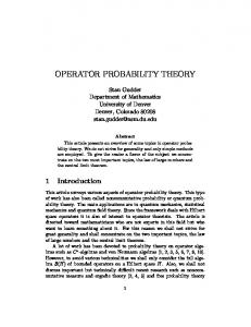
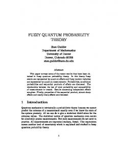


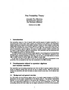


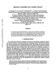


![[PDF] Download Measure Theory and Probability Theory - Google Sites](https://m.moam.info/img/260x300/pdf-download-measure-theory-and-probability-theory_64773dd0097c4737708b7b9a.jpg)
